Investigating the impact of geopolitical risks on the commodity futures

Abstract

This paper examines the effect of real-time global geopolitical risks (GPRs), acts (GPAs), and threats (GPTs) indices on monthly returns and volatility of several American commodity futures. By modeling volatility via an Exponential Generalized Autoregressive Conditional Heteroskedasticity (EGARCH), we provide evidence that GPRs and GPTs do not only impact but trigger adverse effects on the returns of crude oil, gold, platinum, and silver, while GPAs negatively affect the returns of crude oil, heating oil, platinum, and sugar futures. Furthermore, GPTs have a weak positive effect on corn futures volatility. Overall, our findings provide portfolio diversification benefits by showing how the impact of global GPRs, GPAs and GPTs on portfolio returns could be mitigated.

Keywords:

• Geopolitical risks
• geopolitical acts
• geopolitical threats
• commodity futures contracts
• returns and volatility
• EGARCH

PUBLIC INTEREST STATEMENT

Commodity futures contract is an agreement to purchase or sell a predetermined amount of the underlying commodity on a specific price and date in the future. These contracts are significant because they could be used to hedge or speculate an investment position. Some known factors that affect their prices are the weather, and macroeconomic fundamentals. In addition, the geopolitical risks seem to have an impact on their prices. This study examined the impact of geopolitical risks, acts and threats on the commodity futures monthly returns and volatility in the United States of America market. Therefore, we detected that the geopolitical risks and threats negatively affect the returns of the crude oil, gold, platinum, and silver, whereas the geopolitical acts have the same effect on of crude oil, heating oil, platinum, and sugar futures. Lastly, our results determined a weak positive relationship between the geopolitical threats and the corn futures volatility.

1. Introduction

Predominantly, the increased turbulence of our times, as reflected for example, on the stock prices or even on the interest rates volatility, has underlined the necessity for an efficient risk transference via various financial instruments and has led to the development of commodity futures. Indicatively, Hamilton and Wu (2015), in the pre-Covid-19 period, has highlighted that during the recent years, and especially after the Global Financial Crisis (GFC), we have witnessed an extraordinary hike in participation in commodity futures. From a speculation and a hedging point of view, as known, commodity futures contracts are perceived as popular derivative instruments to spread portfolio related risk. The investors use them to achieve risk reduction, portfolio optimisation, and hedging (Bansal et al., 2014; Rallis et al., 2012; Sarafrazi et al., 2014). Consequently, investigating the factors that can affect their prices is important in finance.

The weather, supply/demand imbalances, macroeconomic fundamentals, and the value of the American dollar are found to be the main drivers of returns and volatility of commodities (Brown & Kshirsagar, 2015; Browne & Cronin, 2010; De Gregorio, 2012; Kagraoka, 2016; Matesanz et al., 2014; Tilton et al., 2011; Trostle, 2008; Wu et al., 2020). Taking these traditional driving forces, along with financialization (Masters, 2008; Tang & Xiong, 2012) into commodity pricing models has become an important strand of literature (see indicatively Ji et al., 2019), and it is valuable not only for the practitioners and the academics but for the policy makers as well. Indicatively, according to Apergis et al. (2017), practitioners discern financial market returns and its volatility as the most significant indicators in the portfolio management and capital budgeting decisions, while academics use the financial market shifts in testing the market efficiency theory and to develope realistic asset pricing models (Narayan & Smyth, 2015). The aforementioned, in their turn, could guide the policy makers in setting the policy related framework more effectively.

Another factor that seems to affect the returns of financial markets is geopolitical news and events. For example, the announcement of the Brexit in June 2016, the election of Donald Trump in November 2016, and the nuclear crisis in 2017 in North Korea, had a substantial impact on financial markets (Rose, 2017). Correspondingly, in 2017, on a survey of one thousand investors, the three-quarters of the participants signify that diplomatic and military conflicts have an economic impact (Bouras et al., 2019). This survey concludes that geopolitical risks surpass economic and political uncertainty in the ranking of the factors that influence the economy; a finding that should be empirically tested and it motivates our study. Thus, as Carney (2016) claims, do the economic and policy uncertainty along with geopolitical risks construe an “uncertainty trinity” that has an adverse economic impact? Therefore, is it significant for investors and traders to comprehend if the commodity futures can hedge such shocks or do they exhibit immunity?

However, before we proceed the perception of the measurement of geopolitical risks has to be documented. It is acknowledged that geopolitical risks are identified on a certain part of literature as terror attacks, and are represented through dummy variables in the time series models (indicatively Plakandaras et al., 2019). Notwithstanding, the measurement of geopolitical risks is much broader and challenging to be captured by a dummy variable. Thus, following a rising literature (see, Antonakakis et al., 2017; Balcilar et al., 2016; Bilgin et al., 2018; Gkillas et al., 2020; Hu et al., 2020; Joëts et al., 2017) that has investigated uncertainty, geopolitical risk and extreme events as the driving forces of the commodity prices, and stressed the significance of geopolitical risks in the formulation of financial and macroeconomic cycles, we use the new indices introduced by Caldara and Iacoviello (2018) that measure in real-time global geopolitical risks (GPRs), acts (GPAs), and threats (GPTs).

Subsequently, the availability of these three indices (GPRs, GPAs, GPTs), along with the Economic Policy Uncertainty (EPU) index, and the Volatility Index (VIX), reflecting the financial market uncertainty as well, can assist us in studying simultaneously the aforementioned “uncertainty trinity” (Carney, 2016) by focusing on financial markets overall, and specifically on the futures markets, and hence on commodity futures.

To wrap up, the prime purpose of our research is to shed light on the impact of geopolitical risks, acts and threats on the commodity futures monthly returns and volatility in the United States of America market. The motivation of the research is to extend the aforementioned studies, along with the existing studies that examine the effect of geopolitical risks on stocks and bonds returns (An & Roh, 2018; Bouri et al., 2019; Cheng & Chiu, 2018; Lee, 2018), by investigating the impact of the three geopolitical indices, along with EPU, VIX and various macroeconomic and financial variables simultaneously (including S&P 500 futures, the 10-Year Treasury constant maturity rate (DGS10) and the Trade Weighted United States dollar-major currencies (DTWEXM)), on several commodity futures of various classes.

Therefore, our study, to the best of our knowledge, uniquely includes three geopolitical indices, two policy uncertainty and volatility indices, and thirteen commodity futures, varying from agricultural, energy to precious metals classes obtained from the Chicago Mercantile Exchange (CME) and the Intercontinental Exchange (ICE); namely, in an alphabetical order, the commodity futures are Cocoa, Coffee, Corn, Crude oil, Feeder cattle, Gold, Heating oil, Live cattle, Natural gas, Platinum, Silver, Sugar and Wheat.

In this paper overall, we aim to answer the following research questions: (1) Do GPRs, GPAs, and GPTs affect the trading commodity futures in the CME and ICE?, and if yes, is the affect an adverse one? (2) Do the effects of GPRs, GPAs, and GPTs depend on the class of the commodity futures? Meaning, does it matter if the commodity future is an agricultural, an energy or a precious metals class? and finally, (3) What are the impacts, in terms of signs and magnitude, of GPRs, GPAs, and GPTs on the American commodity futures monthly returns and volatility? To the best of our knowledge, this is the first time that the indices of Caldara and Iacoviello (2018) are used to examine their effects on thirteen American commodity futures markets of three broader classes.

In order to address these questions, we implement several Generalized Autoregressive Conditional Heteroskedasticity (GARCH)-type models, concluding to a robust Exponential GARCH (EGARCH), that incorporates the innovative geopolitical risks, acts, threats (henceforth GPRs, GPAs, GPTs index) indices, capturing a broader array of exogenous global uncertainty. After controlling several variables, the regressions exhibit that GPRs and GPTs negatively affect the returns of precious metals and crude oil. Moreover, we pinpoint that GPTs have a weak positive effect on corn futures volatility, while GPAs negatively influence the returns of crude oil, heating oil, platinum, and sugar futures.

The remainder of the paper is structured as follows: Section 2 discusses the literature on GPRs and financial markets; while, Section 3 presents the data and descriptive statistics. Section 4 describes the methodology, and Section 5 contains the empirical results. Finally, Section 6 concludes.

2. A brief literature review on geopolitical risks and financial markets

In our era, geopolitical information seems to have an impact on financial markets (Gkillas et al., 2020, 2018). It is a different factor compared to the financial market uncertainty, which is captured by the Chicago Board Options Exchange Volatility Index (VIX). Recently, the International Monetary Fund (IMF) and the European Central Bank (ECB) recognise the geopolitical factor as a prominent risk to economic outlook (Plakandaras et al., 2018). Typically, geopolitical risks contain terrorist acts, tensions and wars between states that alter international relations, and the new risks that derive from the escalation of the current events (Caldara & Iacoviello, 2018).

Few studies incorporate the geopolitical indices of Caldara and Iacoviello. Aysan et al. (2019), for example, compute the Bitcoin daily logarithmic returns and price volatility from 2010 to 2018. By applying a Bayesian Graphical Structural VAR model, these authors claim that variations in the GPR index have a predictive power on Bitcoins returns and price volatility. By implementing Quantile-on-Quantile estimations, the results unveil a statistically positive significant relationship between the GPR index with the returns and price volatility of Bitcoin at the upper quantiles. Based on that, Bitcoin can be used as a hedging tool towards geopolitical risks, and specifically in extreme geopolitical events.

Bouri et al. (2019) attempt to detect if the Islamic bonds and equities could hedge geopolitical risks. These authors implement a non-parametric causality-in-quantiles test on monthly data of the GPR, Dow Jones Sukuk, and Dow Jones Islamic World indices from 2005–2017 and 1996–2017, respectively, and find that the Islamic financial instruments are affected by the GPR index. Therefore, they cannot diversify the risk of geopolitical events in investment portfolios.

Balcilar et al. (2018) examine the issue of geopolitical risks on the returns and volatility dynamics in the stock markets of the BRICS countries.¹ They apply a VAR model on significant stock indices monthly data from 1985 for South Africa, 1990 for India, 1993 for China, 1994 for Brazil, and 1998 for Russia with an end date always in 2016. The outcomes imply that India is the most resilient country, while Russia’s stock return and volatility influence higher from geopolitical risks. Bouras et al. (2019) analyse the role of the GPR index on the returns and volatility of eighteen emerging market economies from several continents. They collect monthly data from November 1998 to June 2017 and implement a panel GARCH (1,1) model. The researchers conclude that global geopolitical risks cannot affect stock returns, but the index has a positive impact on equity market volatility.

Al-Yahyaee et al. (2019), using daily data from August 2013 to August 2018, apply a bivariate and multivariate wavelet analysis. They highlight that the GPR index in the United States has predictive power over the volatility and price returns of Bitcoin. Demiralay and Kilincarslan (2019), in their turn, investigate the impact of geopolitical risks on travel and leisure stock indices of different regions. They obtain monthly data from January 1992 to August 2018 and apply classical linear and quantile regression models. Their findings indicate that geopolitical risks have a negative impact on Europe, Global and North America travel and leisure stock returns, primarily when the industry performs poorly. On the contrary, the Asia Pacific index reveals to be resilient to geopolitical events. Moreover, Demir et al. (2018) advocate that GPRs can be the main factor of the diminishing returns of the Turkish Paintings Price Index during the period 2010 to 2016.

Finally, and to wrap up this brief and indicative literature on this area, Antonakakis et al. (2017) and Plakandaras et al. (2019), by implementing a VAR-BEKK-GARCH and TVP-VAR models with different Bayesian methods respectively, provide evidence of a negative relationship between crude oil returns and GPRs.² This is a relationship that we plan to test, by adding to GPRs, GPAs, and GPTs too, and also, apart from that, we extend the research by focusing not only on the impact of geopolitical uncertainty on crude oil, but to twelve more commodity futures of various classes as well.

3. Data and descriptive statistics

We compile monthly data for several commodity futures, continuous contract#1 from the CHRIS-Quandl and Investing.com sites. Also, we collect the commodities spot prices from the Macrotrends site, the World Bank, the United States Energy Information Administration and the United States Department of Agriculture National Agricultural Statistics Service. It has to be noted that spot price is the current quote to instantly purchased and delivered commodity, whereas the futures contract is referred to a predetermined future price and date (Table 1 and 4).

Table 1. Mean equations results

	GPR	GPA	GPT
Crude oil	0.018377**	0.027232***	−0.014804*
	[0.0406]	[0.0018]	[0.0705]
Gold	−0.01069***	−0.004036	−0.01027***
	[0.0078]	[0.2272]	[0.0086]
Heating oil	−0.005343	−0.010332**	−0.003694
	[0.3193]	[0.0245]	[0.4551]
Platinum	0.012266**	−0.008928**	−0.011141**
	[0.0332]	[0.0374]	[0.0358]
Silver	0.012501***	−0.003387	−0.010958***
	[0.0053]	[0.5118]	[0.0068]
Sugar	−0.010686	0.018873***	−0.007225
	[0.3313]	[0.0070]	[0.4866]

The values in bracket are the p values.

(*), (**) and (***) indicated the statistical significance at the 10%, 5% and 1% level.

Table 2. Variance equations results

with the GPR	ω	α	γ	β	κ
Corn futures returns	1.426916***	0.866305***	−0.058842	0.468381***	0.00423
	[0.0022]	[0.0000]	[0.6225]	[0.0001]	[0.1708]
Crude oil futures returns	0.223803	0.449328***	0.049701	0.865686***	0.001511
	[0.2343]	[0.0000]	[0.5421]	[0.0000]	[0.3936]
Gold futures returns	0.248692	0.46648***	0.009632	0.794587***	0.002341
	[0.3341]	[0.0001]	[0.9176]	[0.0000]	[0.3261]
Heating oil futures returns	0.141336	0.626019***	−0.054827	0.826503***	0.002367
	[0.5017]	[0.0000]	[0.5636]	[0.0000]	[0.1447]
Platinum futures returns	0.14916	0.571556***	0.004338	0.826789***	−0.000975
	[0.4918]	[0.0000]	[0.9619]	[0.0000]	[0.6973]
Silver futures returns	0.317473	0.753782***	0.099078	0.770323***	0.002161
	[0.2913]	[0.0000]	[0.2172]	[0.0000]	[0.2630]
Sugar futures returns	0.28604	0.58586***	−0.017873	0.831014***	0.000152
	[0.3055]	[0.0000]	[0.8207]	[0.0000]	[0.9454]

The values in bracket are the p values.

(*), (**) and (***) indicated the statistical significance at the 10%, 5% and 1% level.

Table 3. Variance equations results

with the GPA	ω	α	γ	β	κ
Corn futures returns	1.508312***	0.867784***	−0.055728	0.451428***	0.000127
	[0.0028]	[0.0000]	[0.6477]	[0.0004]	[0.9485]
Crude oil futures returns	0.215796	0.403773***	0.076841	0.875094***	0.000903
	[0.1944]	[0.0000]	[0.3144]	[0.0000]	[0.3069]
Gold futures returns	0.141466	0.450278***	0.024288	0.835082***	0.002011
	[0.5041]	[0.0001]	[0.7908]	[0.0000]	[0.3510]
Heating oil futures returns	0.124755	0.644506***	−0.0328	0.827429***	0.001854
	[0.5263]	[0.0000]	[0.7376]	[0.0000]	[0.1080]
Platinum futures returns	0.131359	0.523767***	0.009882	0.843302***	0.000677
	[0.5140]	[0.0000]	[0.9128]	[0.0000]	[0.6723]
Silver futures returns	0.253223	0.641368***	0.133109	0.810208***	0.001115
	[0.3601]	[0.0000]	[0.1035]	[0.0000]	[0.5138]
Sugar futures returns	0.199177	0.512375***	0.007743	0.862998***	−0.001877
	[0.4049]	[0.0001]	[0.9206]	[0.0000]	[0.3134]

The values in bracket are the p values.

(*), (**) and (***) indicated the statistical significance at the 10%, 5% and 1% level.

Table 4. Variance equations results

with the GPT	ω	α	γ	β	κ
Corn futures returns	1.395948***	0.86838***	−0.057083	0.474512***	0.004697*
	[0.0022]	[0.0000]	[0.6311]	[0.0001]	[0.0948]
Crude oil futures returns	0.225673	0.453561***	0.04475	0.864644***	0.0012
	[0.2334]	[0.0000]	[0.5868]	[0.0000]	[0.4582]
Gold futures returns	0.273478	0.471983***	0.014375	0.785129***	0.002079
	[0.3064]	[0.0001]	[0.8776]	[0.0000]	[0.3853]
Heating oil futures returns	0.148564	0.626451***	−0.05824	0.825007***	0.002072
	[0.4884]	[0.0000]	[0.5383]	[0.0000]	[0.2006]
Platinum futures returns	0.163111	0.584235***	0.011237	0.820052***	−0.001429
	[0.4656]	[0.0000]	[0.9015]	[0.0000]	[0.5355]
Silver futures returns	0.324443	0.744904***	0.096835	0.770424***	0.002024
	[0.2845]	[0.0000]	[0.2290]	[0.0000]	[0.2931]
Sugar futures returns	0.281657	0.590456***	−0.017399	0.83109***	0.000562
	[0.3170]	[0.0000]	[0.8254]	[0.0000]	[0.7877]

The values in bracket are the p values.

(*), (**) and (***) indicated the statistical significance at the 10%, 5% and 1% level.

In the futures market, the difference between the cash price and the futures contract of a specific commodity is known as the basis. Table 5 illustrates the selected futures and the period (Appendix A). The soft commodities and heating oil are raw data from the ICE, and the rest of the data are obtained from the CME. The data are non-adjusted prices based on spot-month continuous contract calculations, and the beginning date of the analysis is based on the data availability.

Figure 1 discloses commodity futures prices over time. It is observed that crude oil and heating oil prices attain their highest peak in 2008, whereas corn in 2012. The precious metals gold and silver reach their highest values in 2011, and platinum in 2008. The 2007–2008 GFC might explain the significant increases in the silver and gold prices since it motivated the investors to purchase safe-haven assets (see, Chkili et al., 2014).

Figure 1. Dynamics of commodity futures prices.

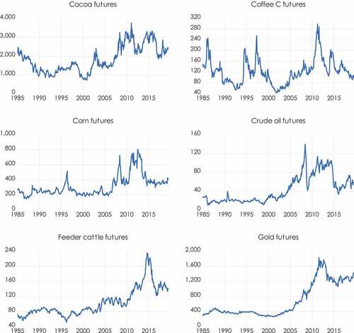
Figure 1. (Continue)

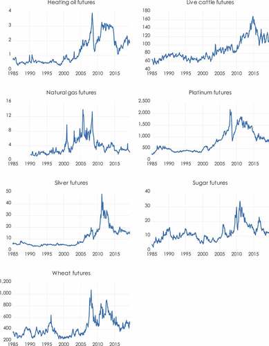
In 2011, the cocoa, sugar and coffee futures demonstrate their maximum prices. On the other hand, the feeder and live cattle peaks are in 2014, while in 2005 and 2008 are the peak years for the natural gas and wheat, respectively. The differences in price patterns can be attributed to factors such as weather conditions, interruption in supply, changes in inventory levels that influence certain commodity futures, while global economic and political events affect other commodities (Ji et al., 2018). Lastly, Figure 2 illustrates the time evolution of the returns.

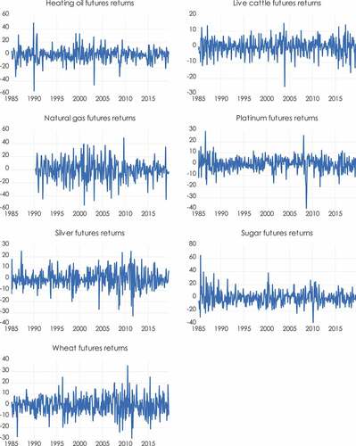
Figure 2. Time-variations in commodity futures returns.

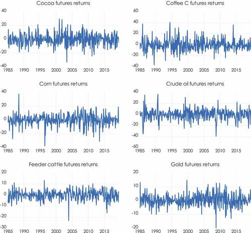
Figure 2. (Continue)

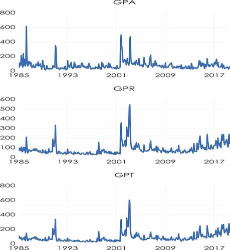
Moreover, the monthly data of the GPR index is obtained from the work of Caldara and Iacoviello for the period January 1985 to July 2019 (Caldara & Iacoviello, 2019). The index is derived by measuring the number of articles that are refereed to geopolitical risks. The counting sources are eleven national and global newspapers; The Washington Post, The New York Times, The Globe and Mail, Chicago Tribune, The Wall Street Journal, Financial Times, The Times, The Boston Globe, The Daily Telegraph, Los Angeles Times, and The Guardian. Afterwards, the index is normalised to the average value of one-hundred in the 2000–2009 period. The automate counting is based on a web search of keywords in the databases of the prementioned newspapers.

The founders formed six groups of keywords. Group one contains words such as “geopolitical risk(s), uncertainty(ies), tension(s), concern(s)” relating a United States involvement and vast regions. Groups two, three, and four consist of words for nuclear tensions, war threats, and terrorist threats, respectively. Groups five and six words look for events that may escalate geopolitical uncertainty, such as acts for the beginning of a war and terrorist acts. Finally, Caldara and Iacoviello constructed through decomposition two other indices, the geopolitical threats index that includes keywords from groups one to four, and the geopolitical acts index that contains groups five and six words (Caldara & Iacoviello, 2018).

The time-variations of these indices are displayed in Figure 3. In March 2003 the GPR and GPT indices exhibit their highest peak. The explanation of this is related to the 2003 invasion of Iraq, also known as the first stage of the Iraq war. Nevertheless, the GPA index escalates in April 1986, and it is correlated with the United States bombing of Libya. Likewise, in September 2001, the GPR and GPA indices present the second highest values that are connected to 9/11 attacks in Lower Manhattan. Lastly, for the GPT index, that period is in September 2002. It is interrelated with the threats on new terrorist attacks in the 9/11 Memorial and the statement of the United States president George Bush to the United Nations about the great danger that Iraq presents to the world. A few days after the presidents’ speech, the United States Congress passed a resolution that authorised the president to use the military forces of the nation whenever “he thinks it is necessary” (Webel & Tomass, 2017).

Figure 3. Dynamics of the GPA, GPR, and GPT indices values over time.

Our study uses the monthly data of the VIX index from January 1986 to December 1989 (using the former calculation method of the index), and thereafter, with the evolution of the VIX, we retrieve the remaining data from January 1990 to July 2019, via the Cboe Global Markets and Yahoo Finance database. As known, this index is created by the Chicago Board Options Exchange and measures the market risk, stress, and fear. The VIX denotes the market’s expectations for volatility over the next thirty days as priced by the S&P 500 index (Fernandes et al., 2014).

Furthermore, we amass the Economic Policy Uncertainty (EPU) index for the United States and the S&P 500 futures, continuous contract#1 from January 1985 to July 2019 through the official site Policy uncertainty.com and CHRIS-Quandl. The former includes news coverage about the policy-related economic uncertainty, economic forecaster disagreement, and tax code expiration data, while the latter is a derivative contract that offers an investment priced based on the expected future value of the S&P 500 index. For the same period, our study garners the 10-Year Treasury constant maturity rate (DGS10) and the Trade Weighted United States dollar-major currencies (DTWEXM) from the Federal Reserve Board.³ The DGS10 is based on the average yield of various Treasury securities that are adjusted to the equivalent of a ten-year maturity. It can be used as a reference point for pricing securities such as corporate bonds. Lastly, the Trade Weighted United States dollar major currencies index is a measurement of the foreign exchange American dollar value compared against certain foreign currencies from countries as Australia, Canada, Euro Area, Japan, United Kingdom, Sweden, and Switzerland.

Table 6 presents the descriptive statistics of the commodity returns and the indices (Appendix B). The corn, crude oil, feeder cattle, gold, heating oil, live cattle, natural gas, platinum, S&P 500, silver futures returns have negative skewness. These results reveal that the distribution has a long left tail, which is skewed to the left. Hence, all the prementioned variables have more observations that are lower compared to the mean. On the contrary, the remaining data have positive skewness. In this case, we identify a right-skewed distribution with a long right tail, which indicates that more observations are higher compared to the mean.

We detect that coffee c futures mean returns are negative, whereas all the other commodity futures returns are positive. Moreover, the values of the standard deviations signpost absolute time-independent volatility of the returns. Thus, it is noticed that natural gas futures have the highest returns’ volatility (15.01) followed by sugar (10.75) and coffee c (10.25). On the other hand, feeder cattle futures have the lowest returns’ volatility (4.18) followed by gold (4.38) and live cattle futures (5.03).

The GPT index average is 84.97, while the GPR and GPA indices are lower at 83.46 and 75.89, respectively. Based on the maximum results, the GPA index has more extreme values than the GPR and GPT index. Notwithstanding, the GPT index has a higher standard deviation than the other two indices, which signifies that the GPT index data are more spread out. Finally, the kurtosis measures the wideness of the distribution, which designates how concentrated the data are around the distribution’s mean.

4. Methodology

Our empirical results are generated from the implementation of a robust GARCH-type (1,1) model. The appropriate estimators for evaluating the goodness of econometric models are the Akaike information criterion (AIC), and the Schwarz Bayesian information criterion (SBIC). Burnham and Anderson (2004) provide arguments in favour of using the AIC over SIC, while according to Kim et al. (2015) and Handika and Chalid (2018) the preferred model is the one with the lower AIC or SIC values and with the highest log-likelihood value. In our paper, we use the AIC’s values to detect the best-fitted model.

As known, the GARCH (1,1) model involves a dual estimation of the conditional mean and variance models. It incorporates heteroskedasticity into the process, captures several structures of conditional variance, and simultaneously estimates many parameters (Bollerslev, 1986). To investigate the commodity futures returns and volatility with the geopolitical risks index, we estimate initially the mean (1) and the variance equations (2)(2) $h_t=\omega +\beta h_{t-1}+\alpha {\epsilon }_{t-1}^2+\kappa {\pi }_{i,t}\left(\mathrm{v}\mathrm{a}\mathrm{r}\mathrm{i}\mathrm{a}\mathrm{n}\mathrm{c}\mathrm{e}\mathrm{e}\mathrm{q}\mathrm{u}\mathrm{a}\mathrm{t}\mathrm{i}\mathrm{o}\mathrm{n}\right)$(2) . Thus, in the mean model (1), our study quantifies the relationship of thirteen commodity futures returns separately with the GPR, GPT, and GPA indices, along with various regressors that are discussed below, and henceforth for the volatility (2), using the GPR, GPT, and GPA indices respectively as well:

(1) $\begin{array}{rl}{R}_t=& C+{\phi }_1{\pi }_{i,t}+{\phi }_{2}VI{X}_t+{\phi }_{3}EP{U}_t+{\phi }_{4}S\mathrm{\&}P{500}_t+{\phi }_5{R}_{t-1}\\ & +{\phi }_{6}DTWEX{M}_t+{\phi }_{7}DGS{10}_t+{\phi }_{8}Spo{t}_t+{\phi }_{9}Spo{t}_{t-1}\\ & +{\phi }_{10}crisi{s}_t+{\epsilon }_t\left(\mathrm{m}\mathrm{e}\mathrm{a}\mathrm{n}\mathrm{e}\mathrm{q}\mathrm{u}\mathrm{a}\mathrm{t}\mathrm{i}\mathrm{o}\mathrm{n}\right)\end{array}$(1)

(2) $h_t=\omega +\beta h_{t-1}+\alpha {\epsilon }_{t-1}^2+\kappa {\pi }_{i,t}\left(\mathrm{v}\mathrm{a}\mathrm{r}\mathrm{i}\mathrm{a}\mathrm{n}\mathrm{c}\mathrm{e}\mathrm{e}\mathrm{q}\mathrm{u}\mathrm{a}\mathrm{t}\mathrm{i}\mathrm{o}\mathrm{n}\right)$(2)

It has to be noted that the following parameters must suffice the non-negativity restraints ω > 0, α, β ≥ 0.

Analytically, R_t is the dependent variable and denotes the logarithmic monthly commodity future return at time period t. The formula for calculating the returns is R_t = ln ($\frac{P_t}{P_{t-1}}$) * 100, where t = 1, …, T, and P_t designates the closing price of the commodity future on month t. Moving to the right side of the equations, π_i,t is the independent variable, and would represent the GPR_t, GPT_t, and GPA_t, when i = 1, i = 2, and i = 3, respectively. As stated above, the variables are the measurements of geopolitical risks, geopolitical threats, and geopolitical acts indices. Furthermore, the VIX_t represents the monthly financial volatility, and the EPU_t the economic and policy uncertainty, while the S&P500_t is the logarithmic monthly future return index. Additionally, the crisis_t is a dummy variable and takes the value of one if the specific tested period experiences a financial crisis (if it is not, then the value is zero). The R_t-1 is the autoregressive AR(1) term or the one month-lag of the commodity future return. The Trade Weighted United States dollar-major currencies and the 10-Year Treasury constant maturity rate indices symbolise by the DTWEXM_t and DGS10_t. The Spot_t and Spot_t-1 denote the spot price of the commodity and the one month-lag of the commodity spot price. Last of all, the terms the φ₁, φ₂, φ₃, φ₄, φ₅, φ₆, φ₇, φ₈, φ_9, and φ₁₀ are the coefficients of the prementioned independent variables, the C is the constant and ε_t is the error term.

The conditional variance typifies as the h_t and ω is the constant term, while the ARCH and GARCH effects are captured by the parameters α and β, respectively. The coefficient α gauges how the volatility responds to market shocks and β computes the impact of new shocks to volatility. They quantify the persistence of the series volatility and if the β value is sufficiently large, the volatility is persistent (Alom et al., 2012).

Moreover, α high value of the coefficient α signifies a sensitive response of the volatility to market movements. If the sum of the coefficients is close to one, then a permanent change will occur in the future values by any shock, which implies a long memory. In other words, the shock is persistent in the conditional variance. The coefficient κ depicts the effects of geopolitical risks, acts, and threats on the variance dynamics of the commodity futures returns. Lastly, it is significant to state that the GARCH (1, 1) process is stationary if the α + β < 1 condition holds (Pan & Chen, 2014).⁴

Glosten et al. (1993) develop a simple extension of the GARCH model the GJR-GARCH (1,1). It differs from the previous model because it has an additional term to contemplate asymmetries. The following function captures the conditional variance:

$h_t=\omega +\beta h_{t-1}+\alpha {\epsilon }_{\mathrm{t}-1}^2+\gamma {\epsilon }_{\mathrm{t}-1}^2{I}_{t-1}+\kappa {\pi }_{i,t}$

The $I_{t-1}$ is a dummy variable that takes the value of unity when ${\epsilon }_{t-1}$< 0, and zero otherwise. Note that γ detects the asymmetric effects in the data, whereas the non-negativity restraints will be ω > 0, α > 0, β ≥ 0, and α + γ ≥ 0 (Saltik et al., 2016).

Additionally, an adverse event has an impact of α + γ, while positive news has an effect of α on the conditional variance. If γ > 0 and statistically significant, then leverage effects exist, and negative shocks will increase the volatility more than positive shocks of the same magnitude. Nevertheless, if γ is negative and statistically significant, then positive shocks will affect the volatility more than adverse shocks. In that case, the model is admissible if the condition α + γ ≥ 0 holds (Pilbeam & Langeland, 2014). For stationarity, the condition (α + β + γ)/2 < 1 must hold (Bampinas et al., 2018).

Nelson (1991) proposes the EGARCH (1,1) which is an alternative asymmetric model. The following variance equation is applied:

$log\left(h_t\right)=\omega +\beta log\left(h_{t-1}\right)+\alpha \left[\frac{{\epsilon }_{t-1}^2}{\sqrt{h_{t-1}}}-\sqrt{\frac{2}{\pi }}\right]+\gamma \frac{{\epsilon }_{t-1}^2}{\sqrt{h_{t-1}}}+\kappa {\pi }_{i,t}$

This is an extension of the GARCH model that considers volatility asymmetry. Specifically, the parameter γ captures the leverage effects, and it must be statistically significant and negative. Correspondingly, the value must be in the following range −1 < γ < 0. In this case, the variance is overresponsive to negative shocks, compared to positive shocks of the same magnitude. Contrarywise, if γ is positive and statistically significant, then the change of h_t is overresponsive to positive shocks. When γ equals to zero, the conditional variance is symmetric to the changes of negative and positive shocks in the same extent (Zomorodian et al., 2016). Lastly, the log form maintains the conditional variance positive even when the parameters are negative.

However, it is recognised that financial time series display non-normality patterns such as excess kurtosis and skewness of the data (Karoglou, 2010). Hereafter, it is imperative to contemplate distributions other than the traditional Gaussian, such as Student’s-t distribution, generalised error distribution, and double exponential distribution (Vrontos, 2012). Consequently, our paper uses the Student’s-t distribution to analyse the data series. Tables 7, 8 and 9 signpost the AIC values and the log-likelihood results for the commodities, from the three GARCH-type models with Student’s-t distribution (Appendix C). Note that all models are applied with the GPR, GPA, and GPT indices. Thus, we conclude that the best fitting model is the EGARCH since it has the lowest AIC values and the highest log-likelihood results⁵ (Appendix D). More precisely, Tables 7 and 8 highlight that six out of thirteen commodities have the lowest AIC values, while seven commodities present maximum log-likelihood results. The results in Table 9 exhibit five and six cases for the AIC values, as well as for maximum log-likelihood, respectively.

5. Empirical results

Initially, we check if the error is normally distributed via the Jarque-Bera test. It has to be noted that the econometric tests are conducted at a = 0.05 level of significance. In all cases, the error term is not normally distributed. The following step is to determine if the time series data are stationary or not, by implementing the Augmented Dickey-Fuller test. In the scenario of the existence of non-stationarity, the data must be transformed into a stationary time series by applying the appropriate order of degree of differentiation. The results pinpoint that not all the variables are stationary in level. Thus, we use the first difference for all variables, and subsequently stationarity condition holds. Finally, to detect whether the conditional heteroscedasticity exists in the commodity futures returns series, we work with the ARCH test method for every R_t model. Our study uses a two-lag length in each test for the regression of squared ordinary least squares residuals. The tests signify that the ARCH effect exists in all the R_t equations. Therefore, EGARCH modelling can be applied for the monthly series.

In order to determine whether there is an absence of serial correlation or autocorrelation in the commodity futures returns series (R_t), we use the correlogram of standardised residuals squared tests. Our study applies a ten-lag test to all the R_t equations to verify the validity of the EGARCH findings. For verification purposes, no autocorrelation should exist in the standardised squared residuals. The null hypothesis indicates the absence of serial correlation, while the alternative states the existence. To detect no autocorrelation in the residuals, the corresponding p values of the Q-Stat should be non-significant in all the lags, at a = 0.05 level of significance. The results present that all models are free from serial correlation. Nevertheless, in the model with GPA, we spot some remaining autocorrelation at lags two, three, four, and five. In this model, the R² decreases approximately by 0.016 in contrast to the other two models. Thus, a portion of model’s adequacy deteriorates.

Moreover, we implement the ARCH test with a ten-lag to detect if conditional heteroscedasticity exists in the residuals of the EGARCH models. The null hypothesis signposts the presence of homoscedasticity in the residuals, which is the required outcome to have valid findings. In all models, we detect homoscedasticity. The last diagnostic test is the Jarque-Bera test. In the test, the null hypothesis states that the standardised residual from the EGARCH models distributes normally. The above statement is the ideal scenario, which is identified in the crude oil and sugar returns models.

The EGARCH (1,1) model is applied in the commodity futures to identify the impact of the GPR, GPA, and GPT indices to their returns (we use student’s-t distribution). Table 1 exhibits the mean equation statistically significant outcomes, and it contains the coefficient values and the p values of geopolitical risks, acts, and threats. Additionally, Tables 2, 3, and 4 present the results from the variance equations. The presence of the ARCH effects, as stated, ratify the appropriateness of the EGARCH model for the selected data.

In the EGARCH model for crude oil returns, the evidence indicates that geopolitical risks, acts, and threats stir the conditional mean of crude oil futures returns. All three indices appear to have a statistically significant impact on the crude oil market. Furthermore, GPRs, GPAs, and GPTs agitate the oil price determination process and the financial markets; all coefficients bear negative signs. Antonakakis et al. (2017) and Plakandaras et al. (2019) also document a negative relationship between oil returns and GPRs.

The variance equations highlight that the ARCH and GARCH effects are statistically significant. Meanwhile, it is evident that the coefficient β is substantially larger than α, which signposts that the changes in the conditional variance are affected more from past variance values, rather than the market shocks. Carnero and Pérez (2018) conclude the same for the ARCH and GARCH effect, but they spot leverage effects at 5% level. In our research we do not have a negative and statistically significant γ, meaning that there is no leverage effect, which is an outcome documented in a relative study by Chevallier and Ielpo (2017) as well. The κ values reveal that geopolitical risks, acts, and threats do not have an impact on crude oil returns’ volatility, despite the negative effect on crude oil futures returns.

Moreover, there is a significant negative relationship between GPRs and gold futures contract returns. We discover the same meticulous relationship for GPTs, whereas GPAs is insignificant. According to Yurdakul and Sefa (2015), the United States dollar value and Brent oil prices affect gold prices. Nyambuu and Tapiero (2018) report that the variables influencing the formulation of gold prices are inflation, geopolitical factors, and the Producer Price index. Lastly, Plakandaras et al. (2018) determine that geopolitical risks possess a significant predicting ability on gold prices. Therefore, there is evidence that geopolitical risks impact gold prices, which eventually disturbs, in their turn, the gold futures contracts.

The coefficients α and β results imply high persistence of gold futures return volatility, and h_t is influenced more from the past volatility. Kang et al. (2017) and Mukherjee and Goswami (2017) report equivalent outcomes for the volatility of gold futures returns. The gold futures returns’ volatility does not shift from geopolitical risks, acts, and threats since the κ values are statistically insignificant. Finally, the fat-tails are captured well by the EGARCH models based on the Student’s-t distribution significance at 1% level.

The heating oil futures returns are not significantly influenced by geopolitical risks and threats. Nonetheless, the model highlights a significant negative impact of geopolitical acts. Baker et al. (2018) detect that the primary factors that affect heating oil are demand/supply, storage costs, crude oil prices, and regional operating costs. Additionally, Karali and Ramirez (2014) state that seasonality is a significant parameter that disturbs the heating oil prices. Consequently, the prementioned factors may also have an impact on the heating oil futures returns.

The variance equations determine that the ARCH and GARCH effects are statistically significant at 1% level of significance. Since the GARCH values are higher than the ARCH, the past volatility values have a greater influence in conditional variance alternations. Chevallier and Ielpo (2017) document that the EGARCH-MN volatility parameters α and β are statistically significant at 1% level for heating oil returns. The κ values are statistically insignificant and suggest that heating futures returns’ volatility is not affected by geopolitical risks, acts, and threats. Lastly, the Student’s-t distribution is significant at 1% level in all models.

The EGARCH models in the platinum futures means returns show a significant negative relationship of geopolitical risks, acts, and threats. Platinum is classified as a precious metal, and similarly to gold commodity futures, the variations of geopolitical risks alter it. Izatt (2016) states that geopolitical issues interrupt platinum and palladium prices, whereas Hammoudeh et al. (2010) identify that geopolitical uncertainty disturbs the platinum returns by implementing a VARMA-GARCH. Subsequently, geopolitical risks seem to affect the platinum futures contracts.

The variance equations from the models with geopolitical risks, acts, and threats indicate a statistical significance of α and β coefficients at 1% level. It is observed that the historical volatility values have a more considerable impact on the h_t shifts. Our findings coincide with the study of Hammoudeh et al. (2010), who investigate via a VARMA-GARCH the conditional volatility of platinum by taking into account geopolitics. In our model, the Student’s-t distribution shows that our population parameters are statistically significant. Also, GPRs, GPAs, and GPTs values from the variance equations are insignificant. Hence, geopolitical risks, acts, and threats influence the conditional mean returns of platinum futures contracts but not its conditional variance.

The mean equations from the models with GPRs and GPTs spot significant negative relationships at 1% level between the silver futures contracts returns with geopolitical risks and threats. Conversely, the value of GPAs has an insignificant impact on silver returns. According to Islam et al. (2018), geopolitical events have an impact on the prices of precious metals. The authors document a significant relationship between silver prices and geopolitical events. Baur and Smales (2018) investigating the impact of geopolitical risks on the returns of silver by implementing an ordinary least squares method, support that geopolitical risks, acts, and threats do not have a significant influence on silver returns.

The variance equations from geopolitical risks, acts, and threats recognise that the ARCH and GARCH effects are statistically significant at 1% level. Our results are consistent with earlier studies by Hammoudeh et al. (2010), Chkili et al. (2014), and Kang et al. (2017). Furthermore, all the κ values are found to be statistically insignificant. Subsequently, these parameters do not affect the conditional volatility of silver futures contracts returns.

The analysis of sugar futures returns indicates that geopolitical risks and threats have an insignificant effect on the sugar futures contracts prices. Contrariwise, the model with GPAs acknowledges a significant negative relationship between geopolitical acts and the sugar returns. Cowen and Tabarrok (2015) advocate that the primary factors that affect sugar prices are supply/demand, climate, U.S. dollar value, and oil prices. The former commodity is recognised as an essential indicator for shaping sugar prices. More specifically, the production of ethanol requires sugar canes, which competes with gasoline in the fuel market. Thus, when oil prices are lower, gasoline and ethanol prices anticipate decreasing in the market. In other words, the demand to produce ethanol declines, and potentially there is an oversupply of sugar. Hence, this could explain the negligible role of geopolitical risks and threats to the sugar futures returns. On the other hand, the connection between oil and sugar prices discloses that geopolitical acts negatively influence the relative commodity futures contracts returns, as it is supported by this research.

The variance equations depict that α and β values are significant at 1% level, for all models. The findings for the ARCH and GARCH effects are similar with Chevallier and Ielpo (2017). The κ values are statistically insignificant, which means that geopolitical risks, acts, and threats do not influence sugar futures returns’ volatility.

Finally, even though geopolitical risks, acts, and threats have an insignificant role in determining the corn futures returns, we find an intrigued result. The GPRs and GPAs parameters have an insignificant effect on the conditional variance of corn futures contracts. Nonetheless, the coefficient of GPTs is statistically significant only at 10% level of significance. Therefore, it is documented, even though this is a statistically weak finding, that geopolitical threats have a positive impact on corn futures returns’ volatility. Additionally, the conditional variance equation from all models shows that the ω, α, and β are positive and statistically significant at 1% level. Based on the values of the ARCH and GARCH effects, we observe that new shocks impact variance more considerable than past volatility (α > β). These results are consistent with earlier findings on returns’ volatility of the corn futures from Kang et al. (2017) and Bohl et al. (2018).

6. Conclusion

This research paper exhibits that geopolitical risks and threats negatively affect the returns of crude oil, gold, platinum, and silver. We find that geopolitical threats have a weak positive effect on corn futures volatility, while geopolitical acts negatively influence the returns of crude oil, heating oil, platinum, and sugar futures. Thus, it is observed that geopolitical risks have a negative relationship with most commodities futures returns.

The rationale is that geopolitics affect commodity markets. Events such as trade wars, closures of central transport routes, conflicts and social unrest cause difficulties in transporting or producing a specific commodity which will lead to a shortage of supply and a rise in price.

Our empirical results have valuable implications for academics, investors, portfolio risk managers, and policymakers. From an academic perspective, the paper sheds light on a new area with a rather limited literature. Researchers and academics can employ the information to enhance their understanding of the correlations between the American commodity futures contracts and geopolitical events. Additionally, the impact of geopolitical risks, acts, and threats to the commodity futures returns and volatility can be used to regulate the efficiency of CME and ICE. Our findings can improve their main functions that are related to risk-management tools and diversification.

On the other hand, investors and portfolio risk managers can utilise the information of GPRs, GPAs, and GPTs to generate higher profits and to design more efficient trading and hedging strategies, particularly in bull rather than bear markets. Bear in mind, that when volatility is interpreted as uncertainty, then it turns into a key input for investment decisions. Furthermore, to price an option, an investor needs to reliable estimate the volatility of the underlying asset. Hence, they should incorporate the parameter of geopolitical events, in their models to compute commodity futures returns and volatility. Lastly, from a policymaker’s viewpoint, the study may contribute in order to implement policies for fostering market stability.

As part of future research, it will be intriguing to investigate the higher-frequency effect of geopolitical risks, acts, and threats to the American commodity futures contracts returns and volatility or either to forecast their returns and volatility. Moreover, it is interesting to monitor the impact of these risks to other countries such as Argentina, Brazil, China, Colombia, India, Indonesia, Israel, Korea, Malaysia, Mexico, Philippines, Russia, Saudi Arabia, South Africa, Thailand, Turkey, Ukraine, and Venezuela, since Caldara and Iacoviello constructed the GPR indices specifically for these nations. Last but not least, by monitoring and modelling the impact of geopolitical events on the commodity futures returns and volatility in the markets can map more effectively the current turbulence and the orientation of our times.

Disclosure statement

No potential conflict of interest was reported by the author(s).

Additional information

Funding

The authors received no direct funding for this research.

Notes on contributors

Sokratis Mitsas

Dr. Petros Golitsis (PhD) is an Assistant Professor in Economics at the City College, University of York Europe Campus, a South-East European Research Centre Research Associate. His research interest covers monetary transmission channels, optimum currency areas, exchange rates and regimes, foreign exchange reserves, and the impact of geopolitical uncertainty on various macroeconomic and financial variables.

Sokratis Mitsas is an Analyst in the Risk Management, Credit Risk, Model Ownership & Data Management Department at ABN AMRO Bank N.V. He received his BA in Business Studies, in specialisation in Accounting and Finance, and MSc in Finance and Banking from the University of Sheffield. His research interest covers the impact of geopolitical uncertainty on various macroeconomic and financial variables.

Dr. Khurshid Khudoykulov is (DSc) is a Professor at department of finance from the Tashkent State University of Economics (TSUE), Tashkent. His research interests focus on asset pricing, capital markets, investment, and the impact of geopolitical uncertainty on various macroeconomic and financial variables.

Notes

1. The BRICS association contains countries from the continents of Brazil, Russia, India, China, and South Africa.

2. Antonakakis et al. (2017) investigate the impact of the GPR index on the oil and stock markets. Using a VAR-BEKK-GARCH model and monthly data of the West Texas Intermediate oil and the Standard & Poor’s (S&P) 500 index from 1899 to 2016, and find that the GPR index has a negative impact primarily on oil returns and volatility, and to a smaller degree on the covariance between oil and stock markets. Plakandaras et al. (2019) using monthly data from January 1985 to June 2017 of the GPR index, WTI crude oil prices, and TVP-VAR models with various Bayesian methods, detect an adverse relationship between geopolitical risks and oil returns in the United States of America.

3. For the details of the 10-Year Treasury constant maturity rate and the Trade Weighted United States dollar-major currencies index, visit the websites of the Federal Reserve Bank of St. Louis (https://fred.stlouisfed.org/series/GS10) and Quandl.com (https://www.quandl.com/data/FRED/DTWEXM-Trade-Weighted-U-S-Dollar-Index-Major-Currencies), respectively.

4. Apart from a GARCH(1,1), we apply various types of GARCH, including GJR-GARCH(1,1) and EGARCH(1,1) (the results are available at the Appendix and upon request).

5. We have applied various robustness related tests, including normality tests, unit root tests, serial correlation tests, whether the conditional heteroscedasticity exists, etc. The most important ones are available and briefly discussed on part 5. The rest are available upon request. Still, it has to be noted here that the presence of the ARCH effects ratify the appropriateness of the EGARCH model for the selected data, which is the best fitted model compared to GARCH and GJR-GARCH. Also, on the variance equations the ARCH and GARCH effects are statistically significant, bearing signs that are consistent with the GARCH constraints. To determine whether there is an absence of serial correlation in the commodity futures returns series (R_t), we use the correlogram of standardised residuals squared tests. All models are free from serial correlation. Lastly, for validity purposes, we apply ARCH tests and detect the presence of homoscedasticity in the EGARCH models residuals.

Appendix A

Table 5. The selected commodity futures

Precious metals class	Starting date	Ending date
Gold	January 1985	July 2019
Platinum	January 1985	July 2019
Silver	January 1985	July 2019
Energy class
Crude oil	January 1985	July 2019
Heating oil	January 1985	July 2019
Natural gas (Henry Hub)	April 1990	July 2019
Agricultural class
Grains-subcategory
Corn	January 1985	July 2019
Wheat	January 1985	July 2019
Livestock and meat-subcategory
Feeder cattle	January 1985	July 2019
Live cattle	January 1985	July 2019
Soft subcategory
Cocoa	January 1985	July 2019
Coffee C (Arabica)	January 1985	July 2019
Sugar	January 1985	July 2019

Appendix B

Table 6. Descriptive statistics

Variables	Mean	Maximum	Minimum	Std. Dev.	Skewness	Kurtosis
Futures returns
Cocoa	0.01	29.69	−32.97	8.45	0.07	3.72
Coffee c	−0.10	40.94	−36.41	10.25	0.53	4.80
Corn	0.09	37.72	−37.66	8.16	−0.37	5.60
Crude oil	0.19	36.89	−39.48	9.69	−0.25	4.97
Feeder cattle	0.16	13.35	−23.04	4.18	−0.52	5.36
Gold	0.37	14.88	−19.66	4.38	−0.01	4.28
Heating oil	0.24	48.52	−54.84	10.21	−0.25	7.34
Live cattle	0.12	14.97	−25.12	5.03	−0.46	4.65
Natural gas	0.10	48.62	−53.81	15.01	−0.20	4.13
Platinum	0.28	29.29	−39.32	6.44	−0.54	7.50
S&P 500	0.68	12.41	−22.83	4.35	−1.02	6.06
Silver	0.23	24.97	−32.65	7.79	−0.10	4.47
Sugar	0.25	64.97	−37.47	10.75	0.87	6.82
Wheat	0.08	35.30	−29.10	8.31	0.07	4.11
Spot prices
Cocoa	1.90	3.53	0.86	0.68	0.53	2.28
Coffee arabica	2.89	6.62	1.17	1.11	0.74	3.52
Corn	3.21	8.03	1.50	1.36	1.54	4.94
Crude oil	43.53	132.83	9.62	31.05	0.95	2.67
Feeder cattle	2.86	6.17	1.63	0.96	0.88	2.86
Gold	680.41	1772.14	256.08	445.87	0.88	2.25
Heating oil	1.63	4.56	0.50	0.87	1.00	2.98
Live cattle	87.13	168.25	49.90	26.53	1.06	3.28
Natural gas	3.76	13.52	1.19	2.19	1.63	6.19
Platinum	800.42	2052.45	260.76	449.30	0.84	2.57
Silver	10.71	42.70	3.65	8.06	1.52	4.91
Sugar	0.27	0.65	0.06	0.11	0.96	3.77
Wheat	183.11	439.72	101.78	67.47	1.23	3.88
Indices
EPU	112.74	284.14	44.78	41.78	1.29	4.92
GPA	75.89	614.91	11.09	64.45	4.16	26.78
GPR	83.46	545.09	23.70	61.29	3.19	18.64
GPT	84.97	602.45	20.23	66.96	3.27	19.57
VIX	19.73	59.89	9.51	7.61	1.84	8.22
Other
DGS10	5.16	11.86	1.50	2.36	0.39	2.30
DTWEXM	89.85	145.18	68.12	12.41	1.18	5.88
Note: The logarithmic monthly returns are used in the table.

Appendix C

Table 7. GARCH-type selection with the GPR index based on the AIC

	GARCH		EGARCH		GJR-GARCH
Commodity futures returns	AIC	Log likelihood	AIC	Log likelihood	AIC	Log likelihood
Cocoa	7.065695	−1400.672	7.070996	−1400.735	7.070673	−1400.67
Coffee	7.433665	−1474.45	7.411787	−1469.063	7.411921	−1469.09
Corn	6.719262	−1331.212	6.72721	−1331.806	6.717663	−1329.891
Crude oil	7.263119	−1440.255	7.273132	−1441.263	7.267837	−1440.201
Feeder cattle	5.992479	−1185.492	5.954105	−1176.798	6.016076	−1189.223
Gold	5.788797	−1140.644	5.772475	−1140.381	5.948435	−1175.661
Heating oil	6.149964	−1217.068	6.170804	−1220.246	6.148458	−1215.766
Live cattle	6.218089	−1227.618	6.224987	−1227.997	6.219778	−1226.956
Natural gas	9.189421	−1587.554	8.451541	−1457.794	8.458151	−1458.947
Platinum	6.409754	−1269.156	6.403066	−1266.815	6.444626	−1275.147
Silver	6.898167	−1367.083	6.882991	−1363.04	6.893317	−1365.11
Sugar	7.415253	−1470.758	7.418546	−1470.419	7.420082	−1470.726
Wheat	7.192937	−1426.184	7.204458	−1427.494	7.197923	−1426.184

Table 8. GARCH-type selection with the GPA index based on the AIC

	GARCH		EGARCH		GJR-GARCH
Commodity futures returns	AIC	Log likelihood	AIC	Log likelihood	AIC	Log likelihood
Cocoa	7.046204	−1396.764	7.072106	−1400.957	7.326741	−1452.012
Coffee	7.43895	−1475.509	7.41893	−1470.496	7.966464	−1580.276
Corn	7.959042	−1579.788	6.73557	−1333.482	6.937015	−1373.872
Crude oil	7.251339	−1437.893	7.26195	−1439.021	7.254479	−1437.523
Feeder cattle	5.975375	−1182.063	5.962391	−1178.459	5.965475	−1179.078
Gold	5.776981	−1142.285	5.783664	−1142.625	5.781968	−1142.285
Heating oil	6.157558	−1218.59	6.158748	−1217.829	6.325295	−1251.222
Live cattle	6.225606	−1229.121	6.227909	−1228.582	6.22473	−1227.946
Natural gas	8.453445	−1459.126	8.450065	−1457.536	8.450907	−1457.683
Platinum	6.414533	−1270.114	6.411518	−1268.509	6.41941	−1270.092
Silver	6.908502	−1369.155	6.897543	−1365.957	6.89909	−1366.268
Sugar	7.382151	−1464.121	7.407792	−1468.262	7.380116	−1462.713
Wheat	7.190074	−1425.61	7.201664	−1426.934	7.195005	−1425.599

Table 9. GARCH-type selection with the GPT index based on the AIC

	GARCH		EGARCH		GJR-GARCH
Commodity futures returns	AIC	Log likelihood	AIC	Log likelihood	AIC	Log likelihood
Cocoa	7.066125	−1400.758	7.071548	−1400.845	7.07111	−1400.758
Coffee	7.4328	−1474.276	7.411514	−1469.009	7.410996	−1468.905
Corn	6.712033	−1329.763	6.72405	−1331.172	6.715825	−1329.523
Crude oil	7.266606	−1440.954	7.277223	−1442.083	7.27147	−1440.93
Feeder cattle	6.383894	−1263.971	5.953945	−1176.766	5.946903	−1175.354
Gold	5.79843	−1140.57	5.772309	−1140.348	6.075081	−1201.054
Heating oil	7.069545	−1401.444	6.173075	−1220.701	6.174774	−1221.042
Live cattle	6.216503	−1227.301	6.224493	−1227.899	6.218874	−1226.775
Natural gas	8.456168	−1459.601	8.453061	−1458.059	8.458857	−1459.071
Platinum	6.410709	−1269.347	6.403465	−1266.895	6.6473	−1315.784
Silver	7.203593	−1428.32	6.882175	−1362.876	7.045171	−1395.557
Sugar	7.417789	−1471.267	7.4198	−1470.67	7.422551	−1471.221
Wheat	7.41147	−1470	7.205238	−1427.65	7.198545	−1426.308

Appendix D

Mean and variance equations

Table

Geopolitical risks: Rt = C + φ1GPRt + φ2VIXt + φ3EPUt + φ4S&P500t + φ5Rt −1 + φ6DTWEXMt + φ7DGS10t + φ8Spott + φ9Spott-1 + φ10crisist + εt (mean equation) log(ht) = ω + βlog(ht-1) + α$[\frac{|{\epsilon }_{\mathrm{t}-1}^2|}{\sqrt{h_{t-1}}}$ -$\sqrt{\frac{2}{\pi }}$] + γ$\frac{{\epsilon }_{\mathrm{t}-1}^2}{\sqrt{h_{t-1}}}$ + κGPRt (variance equation)

Geopolitical threats: Rt = C + φ1GPTt + φ2VIXt + φ3EPUt + φ4S&P500t + φ5Rt −1 + φ6DTWEXMt + φ7DGS10t + φ8Spott + φ9Spott-1 + φ10crisist + εt (mean equation) log(ht) = ω + βlog(ht-1) + α$[\frac{|{\epsilon }_{\mathrm{t}-1}^2|}{\sqrt{h_{t-1}}}$ -$\sqrt{\frac{2}{\pi }}$] + γ$\frac{{\epsilon }_{\mathrm{t}-1}^2}{\sqrt{h_{t-1}}}$ + κGPTt (variance equation)

Geopolitical acts: Rt = C + φ1GPAt + φ2VIXt + φ3EPUt + φ4S&P500t + φ5Rt −1 + φ6DTWEXMt + φ7DGS10t + φ8Spott + φ9Spott-1 + φ10crisist + εt (mean equation) log(ht) = ω + βlog(ht-1) + α$[\frac{|{\epsilon }_{\mathrm{t}-1}^2|}{\sqrt{h_{t-1}}}$ -$\sqrt{\frac{2}{\pi }}$] + γ$\frac{{\epsilon }_{\mathrm{t}-1}^2}{\sqrt{h_{t-1}}}$ + κGPAt (variance equation)

References

- Al-Yahyaee, K., Rehman, M., Mensi, W., Al-Jarrah, I. (2019). Can uncertainty indices predict Bitcoin prices? A revisited analysis using partial and multivariate wavelet approaches. The North American Journal of Economics and Finance, 49(March), 47–24. https://doi.org/10.1016/j.najef.2019.03.019
- Alom, F., Ward, B., & Hu, B. (2012). Modelling petroleum future price volatility: Analysing asymmetry and persistency of shocks. OPEC Energy Review, 36(1), 1–24. https://doi.org/10.1111/j.1753-0237.2011.00204.x
- An, J., & Roh, H. (2018). Measuring North Korean geopolitical risks: Implications for Asia’s financial volatilities. East Asian Policy, 10(3), 41–50. https://doi.org/10.1142/S1793930518000260
- Antonakakis, N., Gupta, R., Kollias, C., & Papadamou, S. (2017). Geopolitical risks and the oil-stock nexus over 1899–2016. Finance Research Letters, 23, 165–173. https://doi.org/10.1016/j.frl.2017.07.017
- Apergis, N., Bonato, M., Gupta, R., & Kyei, C. (2017). Does geopolitical risks predict stock returns and volatility of leading defense companies? Evidence from a nonparametric approach. Defence and Peace Economics, 29(6), 684–696. https://doi.org/10.1080/10242694.2017.1292097
- Aysan, A., Demir, E., Gozgor, G., & Lau, C. (2019). Effects of the geopolitical risks on Bitcoin returns and volatility. Research in International Business and Finance, 47, 511–518. https://doi.org/10.1016/j.ribaf.2018.09.011
- Baker, H., Filbeck, G., & Harris, J. (2018). Commodities: Markets, performance, and strategies. Oxford University Press.
- Balcilar, M., Bonato, M., Demirer, R., & Gupta, R. (2018). Geopolitical risks and stock market dynamics of the BRICS. Economic Systems, 42(2), 295–306. https://doi.org/10.1016/j.ecosys.2017.05.008
- Balcilar, M., Gupta, R., & Pierdzioch, C. (2016). Does uncertainty move the gold price? New evidence from a nonparametric causality-in-quantiles test. Resources Policy, 49, 74–80. https://doi.org/10.1016/j.resourpol.2016.04.004
- Bampinas, G., Ladopoulos, K., & Panagiotidis, T. (2018). A note on the estimated GARCH coefficients from the S&P1500 universe. Applied Economics, 50(34–35), 3647–3653. https://doi.org/10.1080/00036846.2018.1436155
- Bansal, Y., Kumar, S., & Verma, P. (2014). Commodity futures in portfolio diversification: Impact on investor’s utility. Global Business and Management Research: An International Journal, 6(2), 112–121.
- Baur, D., & Smales, L. (2018). Gold and geopolitical risk. SSRN Electronic Journal, 1–25. https://doi.org/10.2139/ssrn.3109136
- Bilgin, M. H., Gozgor, G., Lau, C. K. M., & Sheng, X. (2018). The effects of uncertainty measures on the price of gold. International Review of Financial Analysis, 58(2017), 1–7. https://doi.org/10.1016/j.irfa.2018.03.009
- Bohl, M., Siklos, P., & Wellenreuther, C. (2018). Speculative activity and returns volatility of Chinese agricultural commodity futures. Journal of Asian Economics, 54, 69–91. https://doi.org/10.1016/j.asieco.2017.12.003
- Bollerslev, T. (1986). Generalized autoregressive conditional heteroskedasticity. Journal of Econometrics, 31(3), 307–327. https://doi.org/10.1016/0304-4076(86)90063-1
- Bouras, C., Christou, C., Gupta, R., & Suleman, T. (2019). Geopolitical risks, returns, and volatility in emerging stock markets: Evidence from a panel GARCH model. Emerging Markets Finance and Trade, 55(8), 1841–1856. https://doi.org/10.1080/1540496X.2018.1507906
- Bouri, E., Demirer, R., Gupta, R., & Marfatia, H. (2019). Geopolitical risks and movements in islamic bond and equity markets: A note. Defence and Peace Economics, 30(3), 367–379. doi:10.1080/10242694.2018.1424613.
- Brown, M., & Kshirsagar, V. (2015). Weather and international price shocks on food prices in the developing world. Global Environmental Change, 35, 31–40. https://doi.org/10.1016/j.gloenvcha.2015.08.003
- Browne, F., & Cronin, D. (2010). Commodity prices, money and inflation. Journal of Economics and Business, 62(4), 331–345. https://doi.org/10.1016/j.jeconbus.2010.02.003
- Burnham, K., & Anderson, D. (2004). Multimodel inference: Understanding AIC and BIC in model selection. Sociological Methods & Research, 33(2), 261–304. https://doi.org/10.1177/0049124104268644
- Caldara, D., & Iacoviello, M. (2018). Measuring geopolitical risk. The Fed - International Finance Discussion Papers.
- Caldara, D., & Iacoviello, M., 2019. Geopolitical Risk (GPR) Index [online]. Www2.bc.edu. Available from: https://www2.bc.edu/matteo-iacoviello/gpr.htm#description [Accessed 26th April 2019]
- Carnero, M., & Pérez, A. (2018). Leverage effect in energy futures revisited. Energy Economics, 82(2018), 237–252. doi:10.1016/j.eneco.2017.12.029
- Carney. 2016. Uncertainty, the economy and policy. Speech at the Bank of England (June), pp. 1–16. [online]. Available from: https://www.bankofengland.co.uk/speech/2016/uncertainty-the-economy-and-policy [Accessed 8th September 2019]
- Cheng, C., & Chiu, C. (2018). How important are global geopolitical risks to emerging countries? International Economics CEPII (Centre d’Etudes Prospectives et d’Informations Internationales), a center for research and expertise on the world economy, 156, 305–325. https://doi.org/10.1016/j.inteco.2018.05.002
- Chevallier, J., & Ielpo, F. (2017). Investigating the leverage effect in commodity markets with a recursive estimation approach. Research in International Business and Finance, 39, 763–778. https://doi.org/10.1016/j.ribaf.2014.09.010
- Chkili, W., Hammoudeh, S., & Nguyen, D. (2014). Volatility forecasting and risk management for commodity markets in the presence of asymmetry and long memory. Energy Economics, 41, 1–18. https://doi.org/10.1016/j.eneco.2013.10.011
- Cowen, T., & Tabarrok, A. (2015). Modern principles of economics (3rd ed.). Worth Publishers.
- De Gregorio, J. (2012). Commodity prices, monetary policy, and inflation. IMF Economic Review, 60(4), 600–633. https://doi.org/10.1057/imfer.2012.15
- Demir, E., Gozgor, G., & Sari, E. (2018). Dynamics of the Turkish paintings market: A comprehensive empirical study. Emerging Markets Review, 36(2017), 180–194. https://doi.org/10.1016/j.ememar.2018.04.007
- Demiralay, S., & Kilincarslan, E. (2019). The impact of geopolitical risks on travel and leisure stocks. Tourism Management, 75, 460–476. https://doi.org/10.1016/j.tourman.2019.06.013
- Fernandes, M., Medeiros, M., & Scharth, M. (2014). Modeling and predicting the CBOE market volatility index. Journal of Banking & Finance, 40(1), 1–10. https://doi.org/10.1016/j.jbankfin.2013.11.004
- Gkillas, K., Gupta, R., & Pierdzioch, C. (2020). Forecasting realized gold volatility: Is there a role of geopolitical risks? Finance Research Letters, 35(May), 1–6. https://doi.org/10.1016/j.frl.2019.08.028
- Gkillas, K., Gupta, R., & Wohar, M. (2018). Volatility jumps: The role of geopolitical risks. Finance Research Letters, 27, 247–258. https://doi.org/10.1016/j.frl.2018.03.014
- Glosten, L., Jagannathan, R., & Runkle, D. (1993). On the relation between the expected value and the volatility of the nominal excess return on stocks. The Journal of Finance, 48(5), 1779–1801. https://doi.org/10.1111/j.1540-6261.1993.tb05128.x
- Hamilton, J., & Wu, J. (2015). Effects of index-fund investing on commodity futures prices. International Economic Review, 56(1), 187–205. https://doi.org/10.1111/iere.12099
- Hammoudeh, S., Yuan, Y., McAleer, M., & Thompson, M. (2010). Precious metals–exchange rate volatility transmissions and hedging strategies. International Review of Economics & Finance, 19(4), 633–647. https://doi.org/10.1016/j.iref.2010.02.003
- Handika, R., & Chalid, D. (2018). The predictive power of log-likelihood of GARCH volatility. Review of Accounting and Finance, 17(4), 482–497. https://doi.org/10.1108/RAF-01-2017-0006
- Hu, M., Zhang, D., Ji, Q., & Wei, L. (2020). Macro factors and the realized volatility of commodities: A dynamic network analysis. Resources Policy, 68(July), 101813. https://doi.org/10.1016/j.resourpol.2020.101813
- Islam, J., Islam, R., Islam, M., & Mughal, M. (2018). Economics of sustainable energy. John Wiley & Sons.
- Izatt, R. (2016). Metal sustainability: Global challenges, consequences, and prospects. John Wiley & Sons.
- Ji, Q., Bouri, E., & Roubaud, D. (2018). Dynamic network of implied volatility transmission among US equities, strategic commodities, and BRICS equities. International Review of Financial Analysis, 57, 1–12. https://doi.org/10.1016/j.irfa.2018.02.001
- Ji, Q., Li, J., & Sun, X. (2019). New challenge and research development in global energy financialization. Emerging Markets Finance and Trade, 55(12), 2669–2672. https://doi.org/10.1080/1540496X.2019.1636588
- Joëts, M., Mignon, V., & Razafindrabe, T. (2017). Does the volatility of commodity prices reflect macroeconomic uncertainty? Energy Economics, 68, 313–326. https://doi.org/10.1016/j.eneco.2017.09.017
- Kagraoka, Y. (2016). Common dynamic factors in driving commodity prices: Implications of a generalized dynamic factor model. Economic Modelling, 52, 609–617. https://doi.org/10.1016/j.econmod.2015.10.005
- Kang, S., McIver, R., & Yoon, S. (2017). Dynamic spillover effects among crude oil, precious metal, and agricultural commodity futures markets. Energy Economics, 62, 19–32. https://doi.org/10.1016/j.eneco.2016.12.011
- Karali, B., & Ramirez, O. (2014). Macro determinants of volatility and volatility spillover in energy markets. Energy Economics, 46, 413–421. https://doi.org/10.1016/j.eneco.2014.06.004
- Karoglou, M. (2010). Breaking down the non-normality of stock returns. The European Journal of Finance, 16(1), 79–95. https://doi.org/10.1080/13518470902872343
- Kim, J., Jung, H., & Qin, L. (2015). Linear time-varying regression with a DCC-GARCH model for volatility. Applied Economics, 48(17), 1573–1582. https://doi.org/10.1080/00036846.2015.1102853
- Lee, J. (2018). The world stock markets under geopolitical risks: Dependence structure. The World Economy, 42(6), 1898–1930. https://doi.org/10.1111/twec.12731
- Masters, M. W. (2008, May 20). Testimony before the committee on homeland security and governmental affairs. US Senate.
- Matesanz, D., Torgler, B., Dabat, G., & Ortega, G. J. (2014). Co‐movements in commodity prices: A note based on network analysis. Agricultural Economics, 45(S1), 13–21. https://doi.org/10.1111/agec.12126
- Mukherjee, I., & Goswami, B. (2017). The volatility of returns from commodity futures: Evidence from India. Financial Innovation, 3(1), 1–23. https://doi.org/10.1186/s40854-017-0066-9
- Narayan, S., & Smyth, R. (2015). The financial econometrics of price discovery and predictability. International Review of Financial Analysis, 42, 380–393. https://doi.org/10.1016/j.irfa.2015.09.003
- Nelson, D. (1991). Conditional heteroskedasticity in asset returns: A new approach. Econometrica, 59(2), 347–370. https://doi.org/10.2307/2938260
- Nyambuu, U., & Tapiero, C. (2018). Globalization, gating and risk finance. John Wiley & Sons.
- Pan, B., & Chen, M. (2014). Quasi-maximum exponential likelihood estimation for a non stationary GARCH(1,1) model. Communications in Statistics - Theory and Methods, 45(4), 1000–1013. https://doi.org/10.1080/03610926.2013.851225
- Pilbeam, K., & Langeland, K. (2014). Forecasting exchange rate volatility: GARCH models versus implied volatility forecasts. International Economics and Economic Policy, 12(1), 127–142. https://doi.org/10.1007/s10368-014-0289-4
- Plakandaras, V., Gogas, P., & Papadimitriou, T. (2018). The effects of geopolitical uncertainty in forecasting financial markets: A machine learning approach. Algorithms, 12(1), 1–17. https://doi.org/10.3390/a12010001
- Plakandaras, V., Gupta, R., & Wong, W. (2019). Point and density forecasts of oil returns: The role of geopolitical risks. Resources Policy, 62(October 2018), 580–587. https://doi.org/10.1016/j.resourpol.2018.11.006
- Rallis, G., Miffre, J., & Fuertes, A. (2012). Strategic and tactical roles of enhanced commodity indices. Journal of Futures Markets, 33(10), 965–992. https://doi.org/10.1002/fut.21571
- Rose, J. (2017). Brexit, Trump, and post-truth politics. Public Integrity, 19(6), 555–558. https://doi.org/10.1080/10999922.2017.1285540
- Saltik, O., Degirmen, S., & Ural, M. (2016). Volatility modelling in crude oil and natural gas prices. Procedia Economics and Finance, 38(October 2015), 476–491. https://doi.org/10.1016/S2212-5671(16)30219-2
- Sarafrazi, S., Hammoudeh, S., & Araújo Santos, P. (2014). Downside risk, portfolio diversification and the financial crisis in the euro-zone. Journal of International Financial Markets, Institutions and Money, 32(1), 368–396. https://doi.org/10.1016/j.intfin.2014.06.008
- Tang, K., & Xiong, W. (2012). Index investment and the financialization of commodities. Financial Analysts Journal, 68(6), 54–74. https://doi.org/10.2469/faj.v68.n6.5
- Tilton, J., Humphreys, D., & Radetzki, M. (2011). Investor demand and spot commodity prices. Resources Policy, 36(3), 187–195. https://doi.org/10.1016/j.resourpol.2011.01.006
- Trostle, R. (2008). Global agricultural demand and supply: Factors contributing to the recent increase in food commodity price. Report of USDA Economic Research Service, 0801.
- Vrontos, I. (2012). Evidence for hedge fund predictability from a multivariate Student’s t full-factor GARCH model. Journal of Applied Statistics, 39(6), 1295–1321. https://doi.org/10.1080/02664763.2011.644771
- Webel, C., & Tomass, M. (2017). Assessing the war on terror: Western and middle eastern perspectives (1st ed.). Taylor and Francis.
- Wu, F., Zhao, W. L., Ji, Q., & Zhang, D. (2020). Dependency, centrality and dynamic networks for international commodity futures prices. International Review of Economics & Finance, 67(July 2019), 118–132. https://doi.org/10.1016/j.iref.2020.01.004
- Yurdakul, F., & Sefa, M. (2015). An econometric analysis of gold prices in Turkey. Procedia Economics and Finance, 23(October 2014), 77–85. https://doi.org/10.1016/S2212-5671(15)00332-9
- Zomorodian, G., Barzegar, L., Kazemi, S., & Poortalebi, M. (2016). Effect of oil price volatility and petroleum bloomberg index on stock market returns of tehran stock exchange using EGARCH model. Advances in Mathematical Finance and Applications, 1(2), 69–84. Available at: www.amfa.iau