Forecasting Turkish lira against the US Dollars via forecasting approaches

Abstract

The aim of this study is to predict the Turkish Lira’s exchange rate against the US Dollar by combining models . As a result, the authors include three univariate forecasting models: ARIMA, Naive, and Exponential smoothing, and one multivariate model: NARDL for the first time with Artificial Neural Network model. To the best of our knowledge, it is a unique study to integrate univariate models, ANN with NARDL. The researchers utilize two combination criteria to forecast the Turkish Lira, namely, equal weightage and var-cor. The findings conclude that the combination of NARDL and Naive outperforms all standalone and combined time series techniques. The results indicate that the Turkish Lira’s currency rate against the USD is strongly reliant on recent time-series observations with symmetric and asymmetric behavior of macro-economic fundamentals.

Keywords:

• Projection
• exchange rate changes
• auto-regressive
• naïve
• exponential smoothing
• ANN

PUBLIC INTEREST STATEMENT

The exchange rate plays an important role in the development of any economy; therefore, it is important to have an eye on the future trends of the exchange rates in order to avoid the exchange rate risk in economic transactions. In the case of Turkey, we have observed drastic fluctuation in exchange rate within a few hours, which itself is an exception therefore in this study, we have forecasted the exchange rate by combining different approaches which include Artificial Neural Network, NARDL, ARIMA, Naïve, and Exponential Smoothing via equal-weights and variance-covariance approaches. The results will be helpful to forecast the Turkish Lira in the future to avoid the unwanted variation, which affects the returns and lose the confidence of the traders. The research is helpful to the FOREX market, investors, traders, exporters, importers, central banks, and individuals to make their policies accordingly.

1. Introduction

Since the embracing of the floating exchange system, Economists have taken steps to probe into its relationship with basic macro-economic indicators (Goh et al., 2020). This was due to the significance of these indicators for any country. The literature and researchers testify that success in these macroeconomic indicators could only be achieved if the country can have a competitive exchange rate. This relation is witnessed in developing economies (Hussain et al., 2019). Academic experts devout their focus toward forecasting exchange rates because of its multidirectional benefits. A forecasted exchange rate reduces uncertainty and leads to an efficient decision (AsadUllah et al., 2021a &, 2021b). Hence, the projection of volatility in the currency market is essential to reduce economic loss. A clear-cut forecasting assists in the correct pricing of financial instruments and superior hedging. Value-at-risk models also make use of precise forecasts. Decision-makers of finance and management consider prediction an essential instrument (Majhi et al., 2009; Moosa, 2000). The strength of the economic condition of a country determines its exchange rate. The fluctuation in the exchange rate occurs due to its supply and demand conditions. This volatility acts as a risk for the traders of foreign currency. The precise projection will aid the businesses and government when deciding the policies and setting up business deals that are sensitive to currency rate fluctuations. The changes in convertibility rate govern the decision of bankers, importers, exporters, and currency holders. Therefore, it has a significant effect on the capital flows in the country.

Turkey is the country that is facing major economic issues like trade deficit and shortage of foreign exchange reserves. The Turkish Lira against the US Dollar exchange rate has been witnessing a quick and sharp fluctuation in past few years. Earlier, the volatility of Turkish Lira was under control. At the start of 2012, the Turkish Lira was calculated as 2.366 against the US Dollar and it fluctuates to 4.56 at the end of financial year 2017. The depreciation in Turkish Lira is accounted as 2.2 units only in the above 7 years which is 93%, i.e., approximately 13% per year. After 2017, there is a rapid fluctuation in Turkish Lira value. For example, due to numerous reasons, the Turkish Lira hit all time high, i.e., 20.04 against the US Dollar at 20 December 2021; however, next day, the Turkish Lira appreciates significantly and come back to 12.84. Here, the fluctuation is approximately 35% in just a single day; therefore, it motivates authors to analyze the factors which affects the exchange rate of Turkish Lira.

It is difficult to conclude which method is best to perform the forecasting. Hence, to achieve meaningful conclusions, a variety of forecasting methods are utilized in this paper for example, ARIMA, Naïve, Exponential Smoothing because all the effectiveness of time series could not be extracted though the one non-linear model (Khashei et al., 2009); therefore, we have also included NARDL and Artificial Neural Network model to evaluate the effectiveness of future projection with univariate time series techniques because Kauppi et al. (2020) describe that these techniques give deviating conclusion as a result of an amendment in time series. It is impossible that any model is perfect in all situation; therefore, we have combined all above models as instructed by Poon and Granger (2003). The remaining structure of the paper consists of section 2- Literature review, section 3- Data and Methodology, section 4- Results and Discussion.

2. Literature review

In the past researches related to combining models to estimate the exchange rate, the experts focused a lot on mixing ANN models, time series model and the famous machine-learning models. A variety of time series models were brought together by R. MacDonald and Marsh (1994) to project the USD parity with the pound sterling, Japanese Yen and Deutschemark. The researcher emphasized that the use of multiple models yields a more concrete result of forecasting. Matroushi (2011) projected the combination of two models for forecasting. By using ARIMA-ANN and MLP, the researcher proposed that ARIMA-MLP yields give us improved results compared to other models, whether single or combined.

To assess the cash flows that are performed in foreign currency, and efficient exchange rate forecast is essential. To gauge the positive and negative externalities involved in international business, exchange rate forecasting is necessary. Using the out of sampling methodology, Meese and Rogoff (1983) in one of their studies discovered that random walk models fail to give out lessor forecast errors when the spectrum of forecasting is broadened to more than one year. For more than one more, structural models yield better results than random models. It is acknowledged that the judgment of Meese and Rogoff was concrete, but few researchers (Chinn & Meese, 1995; Mark, 1995; Ronald MacDonald & Marsh, 1997) discovered models that used random walk models and still produced improvised forecasting using out of sample methodology. Ince and Trafalis (2006) analyzed the broad category of currency’s exchange rates for forecasting. The researchers used parametric techniques as well as non-parametric techniques. The line of parametric models consists of VAR, ARIMA models etc., amalgamated with non-parametric techniques such as Artificial Neural Network (ANN). The results produced the judgment that the individual models were not as efficient as the combined models. In one of his research papers, Hogan. (1985) differentiated a variety of structural models with the timed series model. Included in Hogan’s study were the following models: ARIMA model, time series model, and sticky-price model.

Dunis and Chen (2006) performed the task of evaluating the nature of 16 models. The result showed that no model on its own is effective, instead, the “mixed model” wins over all the models. The model that won utilizes Neural Network Regression, volatility and various time series techniques and showed that these models are effective in “mixed modelling”.

Jon Faust et al. (2002) investigated the efficiency of fundamental exchange rate models for real-time projection. Many authors of the new generation (; T Taylor et al. 2001) presented some novel conclusions. They stretched their stance that foundation economic theories are, no doubt, effective but the economic models of exchange rates are not efficient enough to give accurate forecasting results. The reason is that these techniques assume a linear trend exists between the data selected, whereas the data are, in reality, of a non-linear trend. They further demonstrated that the base is in the long-run optimum situation and the economy settles in a non-linear trend (Mahesh, 2005).

Lam et al. (2008) & Altavila and Grauwe (2008) experimented on various significant currencies of the business world. The experiment gave the conclusion that the usage of multiple models yields better results than the usage of the singular model.

Wang et al. (2016) projected the currency parity linking the three-layer ANN model with the Autoregressive integrated moving average model. The process was run on the US/Euro rates for 2010–2013. The outcome shows that the selected linked models performed better than the individual ones. Shahriari (2011) and Nouri et al. (2011) performed the tests which concluded that 20 sets of Naїve and cubic regression techniques produce good forecasting results in combination as compared to use as individual.

In the past evidence of literature writing, it is visible that past authors focused on combining models of ANN, machine learning and time series for the projection of exchange rates. This paper will emphasize combining Univariate Time Series & Non-Linear ARDL Techniques to produce improvised forecasting results. This study will further evaluate that combined models perform better than individual ones or not.

3. Data & methodology

3.1. Data set

In this study, the authors gathered the monthwise data of the Turkish currency, i.e. the rate of Turkish lira against the United Stated Dollars from January of 2011 till December 2019. The rest of the observations prevailing from M1 2020 to M12 2020 were avoided to be used for the in-sample forecasting. The authors used 2011 data from the IMF IFS statistics as the base year, i.e., 2010, to compile input observations for independent variable in the NARDL Co-Integration model. The Monetary Based Rate Of growth, Trade gap, GDP, Cost Of borrowing, Rate Of inflation, Price Of oil, and Gold Prices are all employed as explanatory variables in this research. These factors were chosen considering the substantial correlations between the currency rate and the selected economic determinants.

3.2. Methodological approaches

For the forecast of time series, there exist large models of two types: one being linear and the other non-linear. According to (Khashei et al., 2009) for a linear model, the model predicts subsequent values by taking multiple linear combinations of our sample. Whereas, for the non-linear model, the creation of models was done to question and the idea of linearity is hypothesized in the control and explanatory variables.

3.3. ARMA/ARIMA

Box and Jenkins (1994) method is among the highly applied models for the prediction to forecast values of future. ARIMA model uses values of previous and the present day for estimating future values of a time series. The ARIMA, an integrated model that utilize differenced data, first and second difference, to make the time series stationary. It takes and breaks up the past data into the Auto Regression method. To make an ARIMA model of a given data that we have, an iterative approach was suggested by Box and Jenkins where ARIMA is referred as (a,b,c). “a” defining the autoregressive model’s order, “b” shows the moving average order, and “c” shows the stationary one’s order. In the case where we have a stationary time series, this model will be called as the ARMA model and be written as (a, b).

Joshe et al. (2020) predicted the time series of the INR versus the USD using ARIMA model. The authors resolved that ARIMA (1,1,5) had given the most appropriate outcomes. Al-Gounmein and Ismail (2020) forecast the Jordanian Dinar against USD. The results concluded that better forecasting was given by ARIMA (1,0,1). Deka and Resatoglu (2019) also used the ARIMA procedure to forecast the exchange rate of Turkish vs USD and the results came out to be suitable. ARIMA was also found suitable by Asadullah et al. (2020) for the forecasting of PKR vs USD. Al-Gounmein and Ismail (2020) apply ARMA/ARIMA approach with other combination of models for forecasting the return on stock investment in the case of Saudi Arabia. Humphrey (2015) was used to forecast the value of the Zambian Kuwacha in relation to the US dollar. In order to make their predictions, the authors used data spanning the years 1964 to 2014. According to the researchers, the ARIMA model is better suited for short-term forecasting than it is for long-term speculative speculation because it is more accurate in the short term. Tlegenova (2014) used ARIMA to forecast different exchange rates, and she discovered that it was a successful method. Due to the fact that the MAPE values obtained were less than 5%, the ARIMA model was found to be robust for forecasting of all three exchange rate time series examined.

3.4. NAIVE

In a naive model, most minuscule amounts of effort and alteration of data are used to put together a forecast. The forecast is set to be the value of the past observation: y(t+1) = Y(t) likewise applied in the exponential smoothening model with alpha equal to 1. The naive model is used as standard for models which have the same features such as the ARIMA and exponential smoothing model. For the main part, the naive models used are the random walk, which uses the current value to predict the next period, and seasonal random walk that uses the value from the current period of previous year as a prediction for the same period of the predicted year.

Dunis and Chen (2006) used the Naive method to simulate the USD against the €uro as a metric. The naive model was ranked sixth in estimating the Saudi Riyal to Indian Currency as per Newaz (2008). Khalid (2008) estimated the currency of three nations using the Naive random walk technique.

3.5. Exponential smoothing

The fields of economics and finance use the ES model frequently (Gardner, 1985) as it is valuable for predicting the future values. Brooks (2004) states that this model is different to ARIMA model in which the linear combination used is earlier of the past time series was used to forecast future values. Exponential smoothing of time series data allocates exponentially decreasing weights for the present to the past observations. Simply put, the older the data, the less value (“weight”) the data are given, recent data are considered as more relevant and is allocated more weight. The basic idea of this model is to assume that the future will be more or less the same as the (recent) past.

The single parameter exponential smoothing model is:

$\begin{array}{rl}\mathrm{Y}\mathrm{t}[\mathrm{k}]=& \mathrm{L}[\mathrm{t}]\\ \mathrm{L}[\mathrm{t}]=& \mathrm{a}\mathrm{l}\mathrm{p}\mathrm{h}\mathrm{a}\mathrm{Y}[\mathrm{t}]+[1-\mathrm{a}\mathrm{l}\mathrm{p}\mathrm{h}\mathrm{a}]\mathrm{L}\mathrm{L}[\mathrm{t}-1]\end{array}$

where Y t(k) is the hypothesized values of time series k, the time t in y(t) is values that are observed, and x is the indicater of weighting. The range of scale is from 0 to 1. Higher values of alpha can be interpreted as the influence due to historical knowledge that will eventually be removed and vice versa. The single parameter for the time series is valid and does not have trend and seasonal effects.

Borhan and Hussain (2011) experimented with multiple models, which includes the exponential smoothing forecasting model, to predict the rate of exchange of Takka with USD. The researchers concluded that exponential smoothing provides a more accurate forecast than the other models employed for prediction. Maria and Eva (2011) calculated various models to forecast the speculation of currency rates that are valuable in a different paper. It was found by the researchers that the exponential smoothing model over runs the researchers’ ARIMA model for integration and other models that were used for prediction.

3.6. NARDL

The model of non-linear ARDL which was created by Shin et al. (2014) makes use of the partial sum decomposition that is positive and negative, to capture non-linear and non-symmetric co-integration among the variables and also differentiates among the long- and short-term influence on the dependent variable and independent variable. The NARDL model if compared with other traditional models provides some benefits such as better performance when using small samples to determine the co-integrating relations. NARDL can be applied on regressors that are found to be stationary at the first difference or at a certain level meaning at I(0) or I(1), but we cannot use them to apply on regressors I(2).

Le et al. (2019) investigated the asymmetrical impacts of currency rate changes on trade flows using the NARDL tool. Bahmani-O et al. (2015) also employed the NARDL model to examine the currency rate’s effect. They determined that the forex had an uneven effect on the volatility of the trade balance. Furthermore, Turan and Mesut (2018) examined the current account and concluded that variations in the trade shortage significantly affected the budget deficit. Owing to the stringent application and benefits of the technique discussed previously, the author decided to include the Non-Linear Auto Regressive Distributive Lag (NARDL) strategy in this paper to evaluate the non-linear effect of exchange rate the various explained parameters as discussed in Table 1 and their unit root in Table 2. Finally, Qamruzzaman et al. (2019) used the NARDL approach to examine the non-linear association between the exchange rate and Foreign investment in the context of Bangladesh. The results indicate that these variables exhibit a non-linear connection in the long term.

Table 1. Assessment of explanatory variables

Variables name	Variable	Assessment
Money supply	MS	Stock of money
Interest rate	IR	Rate of central bank
Inflation	INF	Consumer price index
GDP-Real	GDP	IPI
Trade balance	TB	Exports, imports
Foreign reserves	FR	Official foreign reserves
Oil price	OP	Price of crude oil

Table 2. Unit root test—explanatory variables

Variables	Augmented dickey- fuller test		Phillip peron test
	Level	1^st diff	Level	1^st diff
FE	–2.067151	–9.790111	–1.942644	–10.45724
FR	–1.980402	–11.37819	–1.980402	–11.37819
GDP	–1.571611	–1.899766	–9.752516	–
MS	–5.014965	–	–2.805490	–8.559155
INF	0.593596	–6.140452	0.338016	–7.615172
IR	–3.200127	–3.335820	–2.352380	–10.05454
TB	–	–14.61663	–5.171394	–17.47622

3.7. Artificial neural networks for forecasting

Forecasting approaches based on time series data can use as a univariate analysis with the series data as the sole input. Along with the lagged time series, technical, inter-market, or fundamental indicators can be added to multivariate analysis. Multivariate analysis, characterized by non-linearity, data-driven analysis, and generalization, has become a popular and dominant technique in economics and finance, with ANNs serving as the p

ANN is the functional unit of deep learning, and it solves complicated data-driven problems by using ANN that replicates the behavior of the nervous system. After feeding the input data to the NN functions, the data are processed through layers of perceptron, simulating the brain’s ability to detect and discriminate, resulting in output. Deep learning is a subset that falls under the broader umbrella of artificial intelligence. These three fields are inextricably linked, with machine learning and deep learning assisting AI by offering algorithms and natural language processing (NN) to handle data-driven challenges.

ANN has devised a comprehensive tool for estimating and forecasting real, valued, and vector value functions. ANN delivers superior solutions than standard statistical techniques under specific circumstances and then for some kinds of problems. The ANN survey was partially motivated by discovering that biological learning systems are constructed from extraordinarily intricate interconnecting neuron webs. ANNs have been built in approximate analogy from a highly connected sample unit collection. Each unit accepts some real-world inputs (potentially the outputs of other departments) and creates a single, real-world result that others can supply [11].

The multi-layer perceptron is the design of an artificial network of the most prevalent form. The processing component consists of many layers (also termed neurons or nodes). The entry values (input data) at the so-called input layer are sent to the neurons. The input values are evaluated in the individual input layer neurons, and the input neurons in the hidden layers are transferred to the neurons. The system output, which has objectives, is located on the output layer. Independent and dependent variables are known as the input and output variables, respectively.

The corresponding variable for every connection (between neurons) indicates the strength of the relationships, known as weight. The network learns to map the features on the input layer in the output layer by altering consequences in a particular way. This technique is known as the learning or training algorithm [45]. It is an explanation of the process of weight adaptation. ANN research consists of various study methods “such as quick propagation, Conjugate Gradient descent, Quasi-Newton, Levenberg-Marquardt, and backpropagation.”

The input values in the input layer analyze each information row in the learning phase, and all data transfers via links to each neuron in the stored levels. However, the weights of the relevant links multiply the information in this communication. All information from input layer is collected by neurons on the hidden layer and transferred to the next layer via multiple weights linkages using the activation function. Logistic, linear, hyperbolic tangent, sigmoid often used activation functions. “The connection weights in each iteration must be modified according to the error-correction rule to better match the system’s output with the output data. This activity is referred to as network learning or training.”

The supplied knowledge separates into two non-overlapping segments for the network training process: the so-called training and testing groups. Sometimes used to educate the network to require target function, this is generally huge training collection. To accomplish its generalization capacity, i.e., the ability to deduce sensible conclusions regarding the demographic characteristics from the sample characteristics of the training set, the network is next applied to analyze the data in the testing dataset. Finally, just after training but before the testing, the validation set can be utilized to check the network.

3.8. Combination technique

Armstrong (2001) deduced the result from his study of “The combination of forecasts is that you should weigh forecasts equally when you are unsure which approach is the best.” Granger and Ramanathan (1984) proposed a practical alternative way, a linear product of individual forecasts, weighed by the matrix of previous predictions and the direction of previous values as determined by OLS (assuming unbiasedness). Some investigators end up employing non-consistent weights rather than constant, equivalent weights. Deutsch et al. (1994) proposed a time-dependent non-linear weighting scheme in their research by modifying the regiment of models and smoothing the transition of autoregressive (STAR) models. Zhang et al. (2020) combined the machine learning and fundamental models for forecasting the exchange rate. Due to the reasons indicated earlier, the authors incorporate var-cor and the technique of equal weighting into their prediction of the currency rate.

The authors take Industrial Production Index (IPI) as a proxy of GDP due to its extensive application in previous studies. Soybilgen (2019) identifies the Turkish business cycle regime during real time by applying the BBQ model and MS model. In this study, the author employs IPI as a proxy of GDP and states that the IPI and GDP move together in most cases; the contrary behavior is infrequent. Modugno et al. (2016) forecast the Turkish GDP through proposed econometric models. The authors state that the Industrial Production Index (IPI) is positively correlated with the GDP; therefore, it has been used by numerous researchers when they require GDP data in high frequency, i.e., monthly. The author further argues that a significant portion of the service sector consumes by the production sector; therefore, the argument against the reliability of IPI due to the increase of service sector share in GDP is worthless.

4. Results and discussions

To begin with either a uni-variate or multivariate series analysis, this first step is to identify any stationarity issue that may exist in the model i.e. the time series does not own any downward or upward trend. In order to overcome this problem, unit roots are verified by Augmented Dickey Fuller Test and the Phillips Peron test.

The table depicts that FE is not constant at level as indicated by t-statistic value −2.067151 and −1.942644 for ADF and PP test, respectively. However, as we have adjusted the trend by taking the first difference and the t statistic result changed to −9.790111 and −10.45724 for ADF and PP test, respectively, making the series stationary. The Foreign Reserves (FR) is not fixed at level with t-statistic value of −1.980402 for both ADF and PP test, respectively. However, as we have adjusted the trend by taking the first difference, the t statistic value changed to −11.37819 for both ADF and PP test, respectively, making the series stationary.

As we move forward to Turkey’s Gross Domestic product (GDP), we saw that results of PP test show that Turkey’s GDP is stationary at level with t-statistic value of −9.752516, whereas ADF test shows that unit root exists at both level and first difference with t-statistic value of −1.571611 and −1.899766, respectively. Money Supply (MS) of Turkey is stationary at level with ADF test, whereas while performing PP test it became stationary only after taking the first difference making the t-statistic value go from −2.805490 to −8.559155.

For Inflation rate (INF) in Turkey, unit root exists at level as the test statistic values for both ADF and PP test are 0.593596 and 0.338016. However, after adjusting the trend, we can see in the table above that inflation rate became stationary with t statistic values of −6.140452 and −7.615172 for ADF and PP test, respectively. On the other hand, Interest Rate in Turkey remains non-stationary at both level and first difference (t statistic value of −3.200127 and −3.335820, respectively) while performing the ADF test, i.e. the unit root exists. However, with PP test, we can see that unit root does not exist after adjusting the trend as t statistic value went from −2.352380 to −10.05454 making Interest rate in Turkey stationary. Last variable in the table is that of Trade Balance in Turkey where we can see that unit root exists neither at level in PP test (t statistic = −5.171394) nor at first difference while performing both ADF (t statistic = −14.61663) and PP test (t statistic = −17.47622), thus, making the variable stationary.

The ARIMA model findings in Table 3 reveal that the ARMA (2,2) model is a good fit for forecasting the Turkish Lira’s exchange rate versus the USD. The R-squared, Akaike info, and Schwarz criterion scores are 0.014586, −0.348285, and −2.48366. Additionally, Table 3 illustrates the predicting result of the exponential smoothing model. The Akaike Info Criterion was used to identify the appropriate model; hence, in this example, the Winters’ additive trend was identified, and the better model A.I.C yielded a value of 70.06440. The most significant alpha value in the preceding model is 1, indicating that the effect of previous future value trends will have no lasting effect. The null values of Phi, beta and gamma demonstrate that previous and recent remarks about future values are meaningless.

Table 3. ARIMA statistics

Models	Selected models	R-Squared		Akaikeinfo		Schwarz criterion
ARMA/ARIMA	ARIMA(2,2)	0.014586		–0.348285		–0.248366
Exponential smoothing	Trend	α	β	Ø	γ	A.I.C
		1.0000	0.000	----	0.000	70.06440

Table 4 provides an analysis of the NARDL constants, which indicate the connection between the exchange rate and economic indices. The bound test returns a value of 3.459068, more significantly than both the minimum and maximum values, providing a considerable presence of a lasting association. The outcomes suggest that a change in the rate of 1 unit of oil results in an increase in the currency rate of 0.01360 units, indicating that the variation in the exchange rate is minimal.

Table 4. Coefficients of NARD long run

Variables	Probability	Standard error	T-Statistics
FR-POS	0.1090	3.26E-06	–1.629725
FR_NEG	0.1041	2.86E-06	–2.537572
OP_POS	0.4251	0.002963	0.809914
OP_NEG	0.4579	0.747629	0.4579
TB_POS	0.5508	7.37E-06	0.600274
TB_NEG	0.5730	7.49E-06	–0.567076
GDP_POS	0.0564	0.000879	1.949403
GDP_NEG	0.3344	0.000664	–0.973975
GP-POS	0.8056	0.000191	–0.247299
GP_NEG	0.9692	0.000234	0.038831
F-Statistics	3.459068	R-Squared	0.996567
Bound test	3.459063	l0 Bound: 3.350	l1 Bound 2.620
Diagnostic tests		P Value
The Breusch-Godfrey serial correlation LM test		0.5751
The heteroskedasticity test: Harvery		0.1056
The RESET test		0.1187

The F-statistic has a significant p-value which is 0.996567. It is necessary to emphasize that the scholars eliminated the rate of interest and money growth standard rate because incorporating the aforementioned explanatory variables contradicted NARDL’s assumptions. Additionally, Table 4 displays the analytical result values. The negligible values for all three tests demonstrate that the input data set does not exhibit autocorrelation problems or homogeneity of variance. Additionally, the RESET test indicates the model’s adequacy for the study.

Table 5 summarizes the accuracy of three univariate time series models. The findings show that the Naive technique is more effective and promising than other models by 3.23738%. The second-best model is NARDL, which outperforms ARIMA and exponential smoothing methods with an MAPE value of 10.11487 percent. The dominance of Nave demonstrates that the rate of exchange of the Lira vs. USD is mainly determined by recent information.

Table 5. Results of combined models via equal weights and var-cor approaches

ARIMA	Naïve	Exponential Smoothing	NARDL	ANN
4.506	1.8522	4.563	1.390	1.454
	Two-Way Combinations (EW)
AR-ES	AR-N	AR-ND	ES-N	ES-ND
4.534	3.179	2.948	3.207	2.976
AR-ANN	ES-ANN	ND-ANN	N-ANN	N-ND
2.333	1.325	1.333	0.999	1.6211
Three-Way Combinations (EW)
AR-ES-N	AR-ES-ND	ES-N-ND	AR-N-ND	AR-ES-ANN
3.64	3.486	2.601	1.398	1.236
AR-N-ANN	ES-N-ANN	AR-ND-ANN	N-ND-ANN
2.666	3.565	2.222	2.008
Four-Way Combination (EW)			Five-Way Combination (EW)
AR-ES-N-ND	AR-ES-N-ANN	ES-N-ND-ANN	AR-ES-N-ANN
3.64	3.486	2.601	0.8888
	Two-Way Combinations (VC)
AR-ES	AR-N	AR-ND	ES-N	ES-ND
2.342	1.076	1.253	1.218	1.388
AR-ANN	ES-ANN	ND-ANN	N-ANN	N-ND
1.222	1.085	0.764	0.854	0.764
Three-Way Combinations (VC)
AR-ES-N	AR-ES-ND	ES-N-ND	AR-N-ND	AR-ES-ANN
1.638	1.577	1.089	0.987	0.999
AR-N-ANN	ES-N-ANN	ES-N-ND	N-ND-ANN
1.086	1.247	1.089	1.585
Four-Way Combination (VC)			Five-Way Combination (VC)
AR-ES-N-ND	AR-ES-N-ANN	ES-N-ND-ANN	AR-ES-N-ANN
1.232	1.229	0.969	0.854

AR = Autoregressive Distributive Lag Model, N = Naïve, ND = NARDL Model, ES = Exponential Smoothing Model, ANN = Artificial Neural Network, VC = Var-Cor Approach, EW = Equal-Weights Approach.

The findings in Table 5 indicate that the optimum approach for forecasting currency movements under similar criteria weights is a two-way combination of the NARDL and Nave models. Furthermore, it demonstrates the critical role of economic parameters and the previous period’s prognosis in forecasting future currency rates and time-series values.

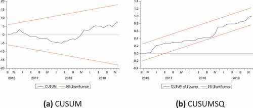
Additionally, Table 5 illustrates individuals’ pairings using the var-cor technique, where the weighting is unlikely to be similar for each model concerning their MAPE. The var-cor and equal weights approaches employ 23 combinations each, including 10 two-way, 9 three-way, 3 four-ways, and 1 five-way combinations. In total, 51 models, which include five individual and forty-six combined models. Additionally, the authors determined that the model was stable by performing the CUSUM and CUSUMQ conditions, as seen in the following Figure 1, demonstrating that the model is stable at a 5% significance level.

Figure 1. CUSUM and CUSUMQ-NARDL.

To conclude, the authors run a total of 51 different techniques for predicting the currency rate where five of which are standalone models, and the remaining are hybrid models integrating multiple methodologies. The combination of NARDL and naïve results to be the best, outperforming all individuals and combining multiple strategies using the equivalent weightage method and the var-cor approach with the lowest MAPE score. Additionally, as Poon and Granger (2003) suggested, incorporating models is critical for economic forecasts. Finally, the combinations of different models validate the authors’ decision to introduce three univariate models of time-driven data.

It is therefore highly recommended to trace the recent observations to forecast the future values of the exchange rate by using Naïve and combination of Naïve and NARDL, which constitutes that the macro-economic fundamentals also play an important role in determining the exchange rate of Turkish Lira. The Turkish government should focus on oil deals that significantly affect their exchange rates.

5. Conclusion

ARMA/ARIMA, exponential smoothing, Nave and one non-linear multivariate model (NARDL) were used to determine the currency rate between the lira and the USD. The authors found that the combined strategy of NARDL and Nave outperformed all other methods, which is why the NARDL model was chosen in this study. Although Nave outperforms than other combinations, NARDL was chosen for this investigation because of its better performance. A few models integrated with each other to achieve superior forecasts than single models, as advocated by the (Poon & Granger, 2001).

5.1. Limitations

The study is limited to Turkish Lira currency only. Three univariate models and one multivariate NARDL model have been applied in this research. Future researchers may alter the applied models and utilize the same methodology to forecast the other currency’s exchange rate. Furthermore, only two combination techniques are used in this study. Results may vary in case of application of other combinations of model techniques.

Disclosure statement

No potential conflict of interest was reported by the author(s).

Additional information

Funding

The authors received no direct funding for this research.

Notes on contributors

Rabia Sabri

Ms. Rabia is a PhD Scholar at PAF-KIET, Karachi and working as a Senior Lecturer at Institute of Business Management. Her research interests include panel data analysis, secondary data and forecasting.

Dr. Abdul Aziz Abdul Rahman is an associate professor at the department of finance and accounting, College of Business, Kingdom University (KU), Bahrain. He has published numerous articles in well-known international journals in accounting, business, and finance.

Dr. Abdelrhman Meero, Associate, Professor, has a Ph.D. Degree in Finance, Bordeaux IV university, Bordeaux, France, 2007. He was the Vice-rector of HIBA (The Higher Institute of Business Administration, Damascus) for 2 years, and he was the Dean of Business College/Kingdom University/Bahrain for five years.

Dr. Liaqat Ali Abro is an advocate in High Court of Pakistan.

Muhammad AsadUllah, PhD Scholar, is the Acting Head of the Department of Department of Professional and Commercial Studies at the Institute of Business Management and a Senior Lecturer.

References

- Al-Gounmein, R. S., & Ismail, M. T. (2020). Forecasting the exchange rate of the jordanian dinar versus the US dollar using a box-jenkins seasonal ARIMA model. International Journal of Mathematics and Computer Science, 15(1), 27–14 http://ijmcs.future-in-tech.net/15.1/R-AlGounmeein.pdf.
- Alshammari, T. S., Ismail, M. T., Al-Wadi, S., Saleh, M. H., & Jaber, J. J. (2020). Modeling and forecasting saudi stock market volatility using wavelet methods. The Journal of Asian Finance, Economics and Business, 7(11), 83–93. https://doi.org/10.13106/jafeb.2020.vol7.no11.083
- Altavila, C., & Grauwe, D. P. (2008). Forecasting and combining competing models of exchange rate determination. Applied Economics, 42(27), 3455–3480. https://doi.org/10.1080/00036840802112505
- Armstrong, J. S. (2001). Combining forecasts. In J. S. Armstrong (Ed.), Principles of forecasting: A handbook of researchers and practitioners (pp. 1–19). KulwerAcademic Publishers.
- Asadullah, M., Ahmad, N., & Dos-Santos, M. J. P. L. (2020). Forecast foreign ExchangeRate: The case study of PKR/USD. Mediterranean Journal of Social Sciences, 11(4), 129–137. https://doi.org/10.36941/mjss-2020-0048
- AsadUllah, M., Bashir, A., & Aleemi, A. R. (2021a). Forecasting exchange rates: An empirical application to Pakistani rupee. Journal of Asian Finance, Economics, and Business, 8(4), 339–347. https://doi.org/10.13106/jafeb.2021.vol8.no4.033
- AsadUllah, M., Uddin, I., Qayyum, A., Ayubi, S., & Sabri, R. (2021b). Forecasting Chinese Yuan/USD Via combination techniques during COVID-19. Journal of Asian Finance, Economics, and Business, 8(5), 221–229. https://doi.org/10.13106/jafeb.2021.vol8.no5.0221
- Bahmani-O, M., Amr, H., & Kishor, N. K. (2015). The exchange rate disconnect puzzle revisited: The exchange rate puzzle. International Journal of Finance & Economics, 20(2), 126–137. https://doi.org/10.1002/ijfe.1504
- Borhan, A. S. M., & Hussain, M. S. (2011). Forecasting exchange rate of Bangladesh – A time series econometric forecasting modeling approach. Dhaka University Journal of Science, 59(1), 1–8 http://journal.library.du.ac.bd/index.php?journal=dujs&page=article&op=view&path%5B%5D=357.
- Box, G. E. P., & Jenkins, G. M. (1994). Time series analysis: Forecasting and control (3rd Upper Saddle, NJ: Prentice-Hall ed.).
- Brooks, C. (2004). Introductory econometrics for finance. Cambridge University Press.
- Chinn, M. D., & Meese, R. A. (1995). Banking on currency forecasts: how predictable is change in money? Journal of International Economics, 38(1–2), 161–178. https://doi.org/10.1016/0022-1996(94)01334-O
- Deka, A., & Resatoglu, N. G. (2019). Forecasting foreign exchange rate and consumer price index with ARIMA model: the case of Turkey. International Journal of Scientific Research and Management, 7(8 1254–1275). https://doi.org/10.18535/ijsrm/v7i8.em01
- Deutsch, M., Granger, C. W. J., & Tera¨svira, T. (1994). The combination of forecasts using changing weights. International Journal of Forecasting, 10(1), 47–57. https://doi.org/10.1016/0169-2070(94)90049-3
- Dunis, D. L., & Chen, Y. X. (2006). Alternative volatility models for risk management and trading: Application to the EUR/USD and USD/JPY rates. Derivatives Use, Trading & Regulation, 11(2), 126–156. https://doi.org/10.1057/palgrave.dutr.1840013
- Faust, J., Rogers, J. H., Swanson, E., & Wright, J. H. (2003). Identifying the Effects of Monetary Policy Shocks on Exchange Rates Using High Frequency Data. Journal of the European Economic Association, 1(5), 1031–1057. http://www.jstor.org/stable/40004851
- Gardner, E. S. (1985). Exponential smoothing: The state of the art. Journal of Forecasting, 4(1), 1–28. https://doi.org/10.1002/for.3980040103
- Goh, T, S., Henry, and Albert, L. (2021) Determinants and prediction of the stock market during COVID-19: Evidence from Indonesia. Journal of Asian Finance, Economics, and Business, 8(1), 1–6. 10.13106/jafeb.2021.vol8.no1.001
- Granger, C. W. J., & Ramanathan, R. (1984). Improved methods of combining forecasts. Journal of Forecasting, 3(2), 197–204. https://doi.org/10.1002/for.3980030207
- Hogan, L. I. (1985). A comparison of alternative exchange rate forecasting models. Bureau of Agricultural Economics.
- Humphrey, F. (2015). Excessive depreciation of the Zambian Kwacha against the US Dollar; firms, household, and government; what is the way forward? International Journal of Applied Research, 1, 1041–1056.
- Hussain. I., Jawad H., Arshad A. K., & Yahya. K. (2019) An analysis of the asymmetric impact of exchange rate changes on G.D.P. in Pakistan: Application of non-linear A.R.D.L. Economic Research-Ekonomska Istrazivanja, 3(1), 3100–3117. 10.1080/1331677X.2019.1653213
- Ince, H., & Trafalis, B. T. (2006). A hybrid model for-exchange rate prediction. Decision Support Systems, 42(2), 1054–1062. https://doi.org/10.1016/j.dss.2005.09.001
- Joshe, V. K., Band, G., Naidu, K., & Ghangare, A. (2020). Modeling exchange rate in india–empirical analysis using ARIMA model. Studia Rosenthaliana (Journal for the Study of Research), 12(3), 13–26 http://www.jsrpublication.com/gallery/2-jsrmarch-s371.pdf.
- Kauppi, H., & Virtanen, T. (2020). Boosting nonlinear predictability of macroeconomic time series. International Journal of Forecasting., 37(1), 151–170. 10.1016/j.ijforecast.2020.03.008
- Khalid, S. M. A. 2008. Empirical exchange rate models for developing economies: A study of Pakistan, China and India References 238. Warwick Business School.
- Khashei, M., Bijari, M., & Raissi, G. A. (2009). Improvement of auto-regressive integrated moving average models using fuzzy logic and artificial neural networks (ANNs). Neurocomputing, 72(4–6), 956–967. https://doi.org/10.1016/j.neucom.2008.04.017
- Lam, L., Fung, L., & Yu, I. (2008). Comparing the forecast performance of exchange rate models. Research Department. Hong Kong Monetary Authority, Working Paper, June.
- Le, H. P., Hoang, G. B., & Dang, T. B. V. (2019). Application of nonlinear autoregressive distributed lag (NARDL) model for analysis of the asymmetric effects of real exchange rate volatility on vietnam’s trade balance. Journal of Engineering and Applied Sciences, 14(13), 4317–4322. https://doi.org/10.36478/jeasci.2019.4317.4322
- MacDonald, R., & Marsh, I. W. (1994). Combining exchange rate forecasts: What is the optimal consensus measure? Journal of Forecasting, 13(3), 313–333. https://doi.org/10.1002/for.3980130306
- MacDonald, R., & Marsh, I. (1997). On fundamentals and exchange rates: a casselian perspective. Review of Economics and Statistics, 79(4), 655–664. https://doi.org/10.1162/003465397557060
- Mahesh, T. K. (2005). Forecasting exchange rate: a univariate out-of-sample approach (box-jenkins methodology. The ICFAI Journal of Bank Management, IV, 60–74.
- Majhi, R., Panda, G., & Sahoo, G. (2009). Efficient prediction of exchange rateswith low complexity artificial neural network models. Expert Systems with Applications, 36(1), 181–189. 10.1016/j.eswa.2007.09.005
- Maria, F. C., & Eva, D. (2011). Exchange-rates forecasting: Exponential smoothing techniques and ARIMA models. The Journal of the Faculty of Economics – Economic, 1(1), 499–508 https://core.ac.uk/download/pdf/6294423.pdf.
- Mark, N. C. (1995). Exchange rates and fundamentals evidence on long-horizon predictability. American Economic Review, 85, 201–218.
- Matroushi, S. (2011). Hybrid computational intelligence systems based on statistical and neural networks methods for time series forecasting: the case of the gold price, Master’s Thesis https://researcharchive.lincoln.ac.nz/handle/10182/3986
- Meese, R. A., & Rogoff, K. (1983). Empirical exchange rate models of the seventies: do they fit out of sample? Journal of International Economics, 14(1–2), 3–24. https://doi.org/10.1016/0022-1996(83)90017-X
- Modugno, M., Soybilgen, B., & Yazgan, E. (2016). Nowcasting Turkish GDP and news decomposition. International Journal of Forecasting, 32(4), 1369–1384. https://doi.org/10.1016/j.ijforecast.2016.07.001
- Moosa, I. A. (2000). Univariate time series techniques. In: I. A. Moosa (Ed.), Exchange rate forecasting: Techniques and applications (pp. 62–97). London: Palgrave Macmillan.
- Newaz, M. K. (2008). Comparing the performance of time series models for forecastingexchange rate. BRAC University Journal, 2, 55–65 http://dspace.bracu.ac.bd/xmlui/handle/10361/438?show=full.
- Nouri, I., Ehsanifar, M., & Rezazadeh, A. (2011). Exchange rate forecasting: A combination approach. American Journal of Scientific Research, 22, 110–118.
- Poon, S., & Granger, C. W. J. (2003). Forecasting volatility in financial markets: A review. Journal of Economic Literature, 41(2), 478–538. https://doi.org/10.1257/.41.2.478
- Poon, S., & Granger, C. W. J. (2003). Forecasting volatility in financial markets: A review. Journal of Economic Literature, 41, 478–538. 10.1257/002205103765762743
- Qamruzzaman, M., Karim, S., & Wei, J. (2019). Do asymmetric relationship exist between the exchange rate and foreign direct investment in bangladesh? evidence from non-linear ARDL analysis. The Journal of Asian Finance, Economics and Business, 6(4), 115–128. https://doi.org/10.13106/jafeb.2019.vol6.no4.115
- Shahriari, M. (2011). A combined forecasting approach to exchange rate fluctuations. International Research Journal of Finance and Economics, 79, 112–119.
- Shin, Y., Yu, B., & Greenwood-Nimmo, M. (2014). Modeling asymmetric co-integration and dynamic multipliers in a nonlinear ARDL framework. In: R. C. Sickles & W. C. Horrace (Eds.), Festschrift in Honor of Schmidt (pp. 281–314). New York: Springer. 10.1007/978-1-4899-8008-3_9.
- Soybilgen, B. (2019). Identifying Turkish business cycle regimes in real time. Applied Economics Letters. https://doi.org/10.1080/13504851.2019.1607243
- Taylor, Mark P., David A. Peel and Lucio Sarno (2001), Nonlinear MeanReversion in Real Exchange Rates: Toward a Solution to the Purchasing Power
- Tlegenova, D. (2014). Forecasting exchange rates using time series analysis: The sample of the currency of Kazakjstan. Statistical Finance, 8, 22–30.
- Turan, T., & Mesut, K. (2018). Asymmetries in twin deficit hypothesis: evidence from CEE Countries. Ekonomický Casopis, 66(1), 580–597 http://cejsh.icm.edu.pl/cejsh/element/bwmeta1.element.cejsh-4a16f6c9-6a7a-4b3e-b9e3-6f057742af2d.
- Wang, S., Tang, Z., & Chai, B. (2016). Exchange rate prediction model analysis based on improved artificial neural network algorithm, 2016th International Conference on Communication and Electronics Systems (ICCES) Coimbatore, India, Coimbatore, 1–5.
- Zhang, Y., & Hamori, S. (2020). The predictability of the exchange rate when combining machine learning and fundamental models. Journal of Risk and Financial Management, 13(48), 1–16. 10.3390/jrfm13030048