The Gini coefficient and discontinuity

Abstract

This article reveals a discontinuity in the mapping from a Lorenz curve to the associated cumulative distribution function. The problem is of a mathematical nature—based on an analysis of the transformation between the distribution function of a bound random variable and its Lorenz curve. It will be proven that the transformation from a normalized income distribution to its Lorenz curve is a continuous bijection with respect to the $L^q$ ([0,1])-metric—for every q ≥ 1. The inverse transformation, however, is not continuous for any q ≥ 1. This implies a more careful attitude when interpreting the value of a Gini coefficient. A further problem is that if you have estimated a Lorenz curve from empirical data,then you cannot trust that the associated distribution is a good estimate of the true income distribution.

Keywords:

• inequality
• probability
• math analysis
• discontinuity

PUBLIC INTEREST STATEMENT

This article deals with the relation between the distribution of income and the measurement of economic inequality in a society. The latter is often expressed as the Gini coefficient, G: the expected difference between two randomly drawn household or individual incomes divided by two times the average income. This division was made to be able to compare the magnitude for different societies. Looking at the income distribution, a reasonable degree of equality in the actual society must imply that the difference between the maximal income and the average income is not too large. If we divide this number by the maximal income, we get a quantity, H, comparable between societies. In this article, it will be shown not only that if H is close to zero, then G is close to zero but also that the opposite is not necessarily true. The most direct consequence is that a small G is not enough to ensure relative economic equality in a society.

1. Introduction

Since the 1960s, economists have widely accepted the Lorenz curve as the tool for deriving measures of income inequality in society, among them the Gini coefficient. The traditional method was to group data in a number of intervals and assume all incomes in an interval to be equal to the average income in the actual interval, Morgan (1962). This gives a lower limit of the “true” Gini coefficient.

The ability in our time to collect and centralize precise data about individual income implies that direct methods are now used to compute the Gini coefficient (see, OECD-IDD, 2017, p. 8). This actual OECD method does not take its offset in the Lorenz curve of observed data. It is based on the relative mean differences of observed income data.¹

In education in the economic sciences, however, the Lorenz curve keeps its position in illustrating the Gini coefficient. Still, in this century, scholars find new ways to derive the approximations made in the 1950s to 70s (see Golden (2008) and Farris (2010)).

At least since 1970, there has been a critical attitude towards the Gini coefficient as a precise measure of inequality (see Atkinson (1970)). Moreover, different proposals using the Lorenz curve have been advanced to give a more multi-faceted idea of inequality. Most influential in that respect were Kakwani (1980), Donaldson & Weymark (1983), and Yitzhaki (1983) with their generalized or higher-order Gini coefficients. Their formulas turned out to be equivalent. In the last twenty years, a variety of new inequality measures have been developed, among them the generalized entropy family of indices. All the way through, we alternatively could use the ratio of the top to bottom shares (see, e.g., Liu and Gastwirth (2020)).

The voice of critics is thus rather comprehensive. The aim of the present article is to point out 2 potential problems working with the Gini coefficient, problems that remain even when using the class of generalized Gini coefficients proposed by Kakwani and others. This is not just another demonstration of the fact that 2 different distributions could have the same Gini coefficient. Rather, we will discover that a small Gini coefficient does not necessarily imply a noticeable degree of equality. Furthermore, if you try to obtain the populations' income distribution from an estimated Lorenz curve—that is solving an inverse problem—then your result might be far from the true distribution. The cause to the problems is not solely due to observed data. It is a discontinuity in the relationship between 'the distribution function and the Lorenz curve for a bounded random variable, which brings trouble.

Consequently, we will in section 2 establish the connection between a cumulative distribution function for a bound, non-negative random variable and its Lorenz curve. It will be proved that any non-decreasing, convex function mapping [0,1] on [0,1] with a non-vertical left-hand tangent in (1,1) will be the Lorenz curve for some bound distribution. the correspondence is 1–1 up to scale. In section 3, the set of normalized income distributions and its subset, the Lorenz curves will be conceived of as subsets in the linear $L^q\left(\left[0,1\right]\right)$-spaces. Thus, for any $q\ge 1$, a metric is present, and it will be established that the Lorenz curve results from its income cdf through a continuous transformation. Traditional measures of inequality, especially the Gini coefficient, appear as distances in $L^q\left(\left[0,1\right]\right)$, and in section 4, we shall see that the inverse transformation, mapping the Lorenz curve to its normalized distribution function, is not continuous. In section 5, we will draw some implications from this fact. The results will be derived in a general manner, which means that there will be no restrictions with respect to the type of bound distribution. This implies that the formal language departs somewhat from prevalent presentation in the economic literature.

2. The transformation mapping a cumulative distribution function to its Lorenz function

A Lorenz curve² is formally a curve in the plane with the property, which for every point belonging to it, $\left(p,y\right),p$, will denote a fraction of a population, while $y$ will denote the relative share of some limited resource or goods, which this fraction possesses. $p$ is explicitly the fraction that has the lowest share of the resource. If we assume that $y$ can never be negative, the curve will contain the points (0,0) and (1,1), and it will be non-decreasing. The associated cumulative distribution function, which has this curve as its graph, will in accordance with the current style also be termed the Lorenz curve. In fact, we have implicitly chosen a statistical model that operates with a large or an indefinite number of members of the population, which is treated as a continuous medium. Furthermore, we will only work with bound and non-negative distributions of the good.

As preliminary results, we have that for any real, non-negative and bound random variable $X$, with cumulative distribution function $F,$ the expectation exists and could be calculated as

(1) $m=E\left(X\right)={\int }_0^{X_{e.s.}}\left(1-F\left(x\right)\right)dx={\int }_0^1{F}^{-1}\left(u\right)du.$(1)

The integral used is the Lebesgue integral, and $X_{e.s.}$ is the essential supremum of $X.$ Note that (1) is valid for any mixture of continuous and atomic distribution functions.

$F^{-1}\left(u\right)$ might not exist as a function as it is not required that $F$ is strictly increasing. So, in this text, $F^{-1}\left(u\right)$ simply means the u-fractile of $F$, formally,

$F^{-1}\left(u\right)=inf\left\{x:F\left(x\right)\ge u\right\}$

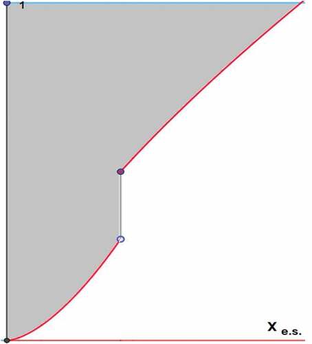
If you are not used to work with $F^{-1}$ in this way, the correctness of the last equality sign in (1) can be justified by Figure 1. The red curve is the graph of $F,$ and the area of the shaded set is both, $E\left(X\right)$ and $\underset{0}{\overset{1}{\int }}{F}^{-1}(u)du,$

Figure 1. The graph of a non-continuous cdf. The area of the shaded set is $\underset{0}{\overset{1}{\int }}{F}^{-1}\left(u\right)du$.

(2) $L\left(p\right)=\frac{1}{m}{\int }_0^p{F}^{-1}\left(u\right)du,p\in \left[0,1\right]\hspace{0.17em}.$(2)

Expression (2) was used by Gastwirth to define the Lorenz curve (see Gastwirth (1971)). Dorfman (1979) in fact generally proves an equivalent result to (2).³

Note that there is no problem with this definition. As $F^{-1}\left(u\right)$ is uniquely determined as a measurable function with up to countably many discontinuities, $L\left(p\right)$ is given in [0.1]. That the Lorenz curve might not be differentiable is merely a consequence of the model (half of me earns half of my income, and my income ranked neighbor to the right-hand side might earn the same as me or (considerably) more). If $F$ is an empirical cdf, then one could object to its application if the sample is small (see Yitzhaki and Schechtman (2013) p 28–29). Let us assume that this is not the case.

Formula (2) defines a mapping, $\mathcal{L}$, of the class of non-negative, finite distribution functions into itself,

$\mathcal{L}:F\left(x\right)\curvearrowright L\left(p\right)$.

Furthermore, (2) ensures that the Lorenz curve, $L,$ will always be convex.

As the third assumption, familiar to the reader, we have that the distribution function of $a\cdot X,a>0$ is given by $F_{aX}\left(x\right)=F_X\left(\frac{x}{a}\right).$ We therefore conclude that

(3) $\mathcal{L}\left(F_{aX}\right)=\frac{1}{m}\hspace{0.17em}{\int }_0^p{F_X}^{-1}\left(u\right)du.$(3)

We will now determine the preimage of an arbitrary Lorenz curve, $L.$ Formula (3) means that for every $a>0,$ $F_{aX}$ will belong to the same preimage as $F_X.$

Equation (2)(2) $L\left(p\right)=\frac{1}{m}{\int }_0^p{F}^{-1}\left(u\right)du,p\in \left[0,1\right]\hspace{0.17em}.$(2) is equivalent to

$m\cdot L(p)=\underset{0}{\overset{p}{\int }}{F}^{-1}(u)du$

(4) $\iff m\cdot l(p)=F^{-1}(p).$(4)

Here, $l\left(p\right)$ is the density function corresponding to $L\left(p\right)$, uniquely determined almost everywhere.

Note that $l\left(p\right)$ is non-decreasing, and because of that, its inverse function will exist in the sense explained above.

In order that $X$ is bound, $F^{-1}\left(1\right)$ must be the finite number $X_{e.s.}$ Consequently, we have

Theorem 2.1

A non-negative random variable is bound if, and only if, the Lorenz curve associated with it has a non-vertical left-hand tangent in the point (1,1). The slope of this tangent is $\frac{X_{e.s.}}{m}$

Equation (4)(4) $\iff m\cdot l(p)=F^{-1}(p).$(4) is equivalent to

$(m\cdot l{)}^{-1}(x)=F(x)$

$\iff l^{-1}\left(\frac{x}{m}\right)=F\left(x\right).$

So, for any fixed $m$ and any given $L$—without a vertical left-hand tangent in (1,1)—$F$ as a cumulative distribution function will be uniquely determined for $x\in \left[0,X_{e.s.}\right].$ We can arrive at the below conclusion:

If the cumulative distribution function $F_X$ for some non-negative, finite random variable $X$ is in the preimage, with respect to the mapping $\mathcal{L},$ of a Lorenz function $L$, the preimage will be exactly $\{F_{aX}:a>0\}$. Thus, we have that

Theorem 2.2

Any finite non-negative distribution function—up to scale—is determined by its Lorenz curve. If the expectation or essential supremum is known, the distribution function is uniquely given.

Formula (4) and Theorem 2.2 were proved by Lambert (1990), p 40–41, in the case of $F$ being differentiable and strictly increasing. In the present context, no results depend on the existence of a density function for the actual distribution function.

We realize that, from now on, we only have to look at the normalized random variable,

$Y=\frac{1}{X_{e.s.}}\cdot X$

when we are working with Lorenz functions for finite random variables. We achieve that $Y\in [0,1]$ and that the transformation

$\mathcal{L}:F_Y\to \frac{1}{m}{\int }_0^p{F_Y}^{-1}\left(u\right)du$

is an injection of the class of distribution functions for normalized non-negative random into itself. Remark: Note that for the graph of $L,$ by Theorem 2.1, the left-hand tangent in (1,1) has a slope of $\frac{1}{m}$, where $m$ is the expectation of $Y.$

Let us illustrate what we found with an example: Suppose that in a given situation,

$L(p)=\left\{\begin{array}{cc}{p}^2& \mathrm{f}\mathrm{o}\mathrm{r}p\in [0,0.5]\\ 1.5(p-1)+& 1\mathrm{f}\mathrm{o}\mathrm{r}p\in ]0.5,1]\end{array}\right.$

and that $m=2.$

As

$l(p)=\frac{1}{2}\cdot F^{-1}(p)$

we get

$F^{-1}\left(p\right)=\left\{\begin{array}{c}4p\mathrm{f}\mathrm{o}\mathrm{r}p\in \left[0,0.5\right]\\ 3\mathrm{f}\mathrm{o}\mathrm{r}p\in \left]0.5,1\right]\end{array}.\right.$

Hence,

$\mathrm{F}(\mathrm{x})=\left\{\begin{array}{c}0.25xforx\in \left[0,2\right[\\ 0.5forx\in \left[2,3\right[\\ 1forx=3\end{array}\right.$

It is the unique solution for $F$ in this situation.

As a random variable, $X,$ with this distribution function $F,$ has the maximal value of 3, and the normalized random variable is $Y=\frac{X}{3}.Y$ has the distribution function,

$F_Y(\mathrm{x})=\left\{\begin{array}{c}0.75\mathrm{x}\mathrm{f}\mathrm{o}\mathrm{r}\mathrm{x}\in [0,\frac{2}{3}[\\ 0.5\mathrm{f}\mathrm{o}\mathrm{r}\mathrm{x}\in [\frac{2}{3},1[\\ 1\mathrm{f}\mathrm{o}\mathrm{r}\mathrm{x}=1\end{array}\right.$

We will denote this class of distribution functions for normalized random variables $NCDF,$ Normalized Cumulative Distribution Functions.

From the way we constructed $Y,$ it is essential that any member of $NCDF$ fulfills that

$x<1\iff F_Y\left(x\right)<1.$

We know that $L=\mathcal{L}\left(F\right)$ is a convex function that maps [0,1] on [0,1]. From Theorem 2.1, we further know that $L$ cannot have an infinite left-hand derivative at $x=1.$ But will any convex function with the domain and range [0,1] be the $\mathcal{L}$-image of some member of $NCDF$ if it only has finite left-hand derivatives?

In the strict sense of convex function, the answer must be no, because the $\mathcal{L}$-image will have to be a distribution function. Consider therefore a convex nondecreasing function $f,$ mapping [0,1] on [0,1], satisfying that $\underset{t\to 1_{-}}{lim}\frac{f\left(1\right)-f\left(t\right)}{1-t}$ is a finite number. We denote this class of functions $CCDF,$ Convex Cumulative Distribution Functions. Every member of $CCDF$ must be continuous.

If $c\in \left]0,1\right[$ then,

$\alpha \left(t\right)=\frac{f\left(c\right)-f\left(t\right)}{c-t},t\in \left[0,1\right],t\ne c$

will be a non-decreasing and non-negative function,⁴ and hence, $\alpha \left(c-\right)=\underset{t\to c-}{lim}\alpha \left(t\right)$ and $\alpha \left(c+\right)=\underset{t\to c+}{lim}\alpha \left(t\right)$ exist and

$\alpha \left(c-\right)\le \alpha \left(c+\right).$

So, $f$ is differentiable from both the left and the right in any point in [0,1] and $f{{ }^{\mathrm{\prime }}}_{-}\left(c\right)\le f{{ }^{\mathrm{\prime }}}_{+}\left(c\right).$ $f$ must be differentiable almost everywhere in [0,1] for the following reason: The set of points fulfilling

$f{{ }^{\mathrm{\prime }}}_{-}\left(c\right)<f{{ }^{\mathrm{\prime }}}_{+}\left(c\right)$

is at most of numerable cardinality, because if we define

$g(x)=\left\{\begin{array}{c}{f}^{\prime }(x)\mathrm{i}\mathrm{f}f\mathrm{i}\mathrm{s}\mathrm{d}\mathrm{i}\mathrm{f}\mathrm{f}\mathrm{e}\mathrm{r}\mathrm{e}\mathrm{n}\mathrm{t}\mathrm{i}\mathrm{a}\mathrm{b}\mathrm{l}\mathrm{e}\mathrm{i}\mathrm{n}x\\ f^{\prime }\mathrm{\_}(x)\mathrm{i}\mathrm{f}f\mathrm{i}\mathrm{s}\mathrm{n}\mathrm{o}\mathrm{t}\mathrm{d}\mathrm{i}\mathrm{f}\mathrm{f}\mathrm{e}\mathrm{r}\mathrm{e}\mathrm{n}\mathrm{t}\mathrm{i}\mathrm{a}\mathrm{b}\mathrm{l}\mathrm{e}\mathrm{i}\mathrm{n}x\end{array}\right.$

$g$ will be non-decreasing in [0,1] and therefore continuous almost everywhere. So, in this way, we found that $f\left(t\right)=\underset{0}{\overset{t}{\int }}g\left(x\right)dx$ on [0,1].

We can identify $g$ with $k\cdot F^{-1}$, the inverse function to a member of $NCDF,$ multiplied by a constant of value $g\left(1\right)$, which, in fact, equals $\frac{1}{m}$, with $m$ being the expectation associated with $F.$ Thus, any member of $CCDF$ is the $\mathcal{L}$-image of a member of $NCDF$.

So far, our investigation has shown the following:

Theorem 2.3

The mapping

$\mathcal{L}:F\to \frac{1}{m}\cdot {\int }_0^p{F}^{-1}\left(u\right)du$

is a bijection of the class $NCDF$ on the class $CCDF.$

Thus, any member of $CCDF$ will be the Lorenz curve for some finite cdf.

3. Convergence of sequences in NCDF and CCDF

$NCDF$ is a subset of the Banach spaces $L^q\left(\left[0,1\right],\lambda \right)$⁵ for every $q\in \left[1,\mathrm{\infty }\right],$ with $\lambda$ being the Lebesgue measure. $NCDF$ and $CCDF$ can now be conceived of as metric spaces—the metric of course induced by $L^q\left(\left[0,1\right],\lambda \right)$. Neither of them is complete, which can be seen in the following example. Let

$F_n\left(x\right)=\{\begin{array}{c}1-\frac{1}{n}\mathrm{f}\mathrm{o}\mathrm{r}x\in \left[0,1\right[\\ 1\mathrm{f}\mathrm{o}\mathrm{r}x=1\end{array}.$

Then, $\left\{F_n\right\}$ is a Cauchy sequence in the space $NCDF$ for any of the metrics in $L^q\left(\left[0,1\right],\lambda \right),q\in \left[1,\mathrm{\infty }\right].$

Since

${∥1-F_n∥}_q={\left({\int }_0^1{\left|1-F_n\left(x\right)\right|}^{q}dx\right)}^{\frac{1}{q}}=\frac{1}{n}\to 0forn\to \mathrm{\infty },$

$\left\{F_n\right\}$ must converge to 1 in the $L^q$-metric, $q<\mathrm{\infty }$. In the $L^{\mathrm{\infty }}$-metric—the supremum norm—the convergence is obvious. Function 1 on [0,1] is certainly not in $NCDF.$

The $\mathcal{L}$-image of $\left\{F_n\right\}$ is the sequence $\left\{n\left(p-\left(1-\frac{1}{n}\right)\right)\cdot 1_{\left[1-\frac{1}{n},1\right]}\left(p\right)\right\}.$ It is a Cauchy sequence in the $L^q$-metric for any real $q\ge 1,$ because the distance between numbers $n$ and $m$ is less than ${\left|\frac{m-n}{2mn}\right|}^{\frac{1}{q}}$, which shrinks to zero with increasing $n$ and $m$ $.$ The limit of the sequence will be

$F(p)=\left\{\begin{array}{c}0forp\in \left[0,1\right[\\ 1forp=1\end{array}\right.$

Although $F$ is a member of $NCDF,$ and although it is convex in $\left[0,1\right]$, it cannot be in $CCDF$, because this set contains exclusively continuous functions. In the $L^{\mathrm{\infty }}$-metric, the $\mathcal{L}$-image of $\left\{F_n\right\}$ is not even a Cauchy sequence.

We will now examine to which extent convergence of a sequence in $NCDF$ implies convergence in $CCDF$ of its $\mathcal{L}$-image.

Lemma 3.1

Given that $F,G\in NCDF$, if we name the expected values connected with $F$ and $G$, respectively,$m_F$ and $m_G$, then

$|m_G-m_F|\le {∥F-G∥}_1$

Proof:

$\left|m_G-m_F\right|=\left|{\int }_0^1\left(1-G\left(x\right)\right)dx-{\int }_0^1\left(1-F\left(x\right)\right)dx\right|$

$=\left|\underset{0}{\overset{1}{\int }}\left(F\left(x\right)-G\left(x\right)\right)dx\right|\le \underset{0}{\overset{1}{\int }}\left|F\left(x\right)-G\left(x\right)\right|dx.$

Now, let $\left\{F_n\right\}$ be a sequence in $NCDF.$

At first, we demand that $\left\{F_n\right\}$ converges to $F$ belonging to $NCDF$ in the $L^{\mathrm{\infty }}\left(\left[0,1\right],\lambda \right)$-metric. Let $m_n$ and $m$ be the expected values connected with $F_n$ and $F,$ respectively.

Now,

${\left|\left|\mathcal{L}\left(F_n\right)-\mathcal{L}\left(F\right)\right|\right|}_{\mathrm{\infty }}=\underset{p\in \left[0,1\right]}{sup}\left|\frac{1}{m_n}\underset{0}{\overset{p}{\int }}{F}_n^{-1}\left(u\right)du-\frac{1}{m}\underset{0}{\overset{p}{\int }}{F}^{-1}\left(u\right)du.\right|$

We see that

${\left|\left|\mathcal{L}\left(F_n\right)-\mathcal{L}\left(F\right)\right|\right|}_{\mathrm{\infty }}\le \frac{\left|m-m_n\right|}{m\cdot m_n}\underset{0}{\overset{1}{\int }}{F}_n^{-1}\left(u\right)du+\frac{1}{m}\underset{0}{\overset{1}{\int }}\left|F_n^{-1}\left(u\right)-F^{-1}\left(u\right)\right|du.$

As a consequence of Lemma 3.1, $m_n\to mforn\to \mathrm{\infty },$ which means that the first term shrinks to 0 as $n$ increases.

For 2 members of $NCDF,$ $G$ and $H$, we consider

${∥G-H∥}_1={\int }_0^1\left|G\left(x\right)-H\left(x\right)\right|dx.$

But this is exactly identical to $\underset{0}{\overset{1}{\int }}\left|G^{-1}\left(u\right)-H^{-1}\left(u\right)\right|du,$as visualized in figure 2. As $\underset{0}{\overset{1}{\int }}\left|F_n\left(x\right)-F\left(x\right)\right|dx$$<\underset{x\in \left[0,1\right]}{\mathrm{s}\mathrm{u}\mathrm{p}\left|F_n\left(x\right)-F\left(x\right)\right|,}$we conclude $\frac{1}{m}\underset{0}{\overset{1}{\int }}\left|{F_n}^{-1}\left(u\right)-F^{-1}\left(u\right)\right|du\to 0$for $n\to \mathrm{\infty }.$

Figure 2. The graph of 2 members of $NCDF,$ named $G$ and $H.$ The area of the shaded set is ${\left|\left|G-H\right|\right|}_1.$

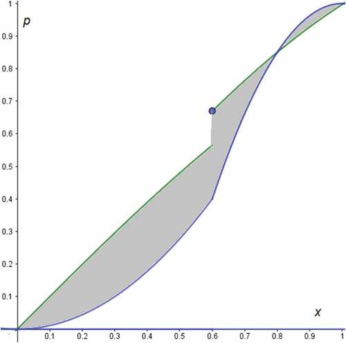
So, ${\left|\left|\mathcal{L}\left(F_n\right)-\mathcal{L}\left(F\right)\right|\right|}_{\mathrm{\infty }}\to 0$

whenever ${\left|\left|F_n-F\right|\right|}_{\mathrm{\infty }}\to 0.$

Next, we let $\left\{F_n\right\}$ converge to $F$ belonging to $NCDF$ in the $L^1\left(\left[0,1\right],\lambda \right)$-metric and look at

$\parallel \mathcal{L}\left(F_n\right)-\mathcal{L}\left(F\right){\parallel }_1=\underset{0}{\overset{1}{\int }}\left|\frac{1}{m_n}\underset{0}{\overset{p}{\int }}{F}_n^{-1}\left(u\right)du-\frac{1}{m}\underset{0}{\overset{p}{\int }}{F}^{-1}\left(u\right)du\right|dp$

With an argument similar to the above one, we get that

$\parallel \mathcal{L}\left(F_n\right)-\mathcal{L}\left(F\right){\parallel }_1\le \underset{0}{\overset{1}{\int }}\frac{\left|m-m_n\right|}{m\cdot m_n}\underset{0}{\overset{1}{\int }}{F}_n^{-1}\left(u\right)dudp+\underset{0}{\overset{1}{\int }}\left|\frac{1}{m}\underset{0}{\overset{p}{\int }}\left(F_n^{-1}\left(u\right)-F^{-1}\left(u\right)\right)du\right|dp,$

Again, the first term will shrink to zero as $n$ increases. The second term will be equal to or lesser than

$\frac{1}{m}\underset{0}{\overset{1}{\int }}\underset{0}{\overset{p}{\int }}\left|F_n^{-1}\left(u\right)-F^{-1}\left(u\right)\right|dudp=\frac{1}{m}\underset{0}{\overset{1}{\int }}\underset{u}{\overset{1}{\int }}\left|F_n^{-1}\left(u\right)-F^{-1}\left(u\right)\right|dpdu,$

where we switched the order of integration. The last expression will be less than

$\underset{0}{\overset{1}{\int }}\left|F_n^{-1}\left(u\right)-F^{-1}\left(u\right)\right|du\to 0forn\to \mathrm{\infty }.$

So,

${\left|\left|F_n-F\right|\right|}_1\to 0\Rightarrow {\left|\left|\mathcal{L}\left(F_n\right)-\mathcal{L}\left(F\right)\right|\right|}_1\to 0.$

We now face the case where $\left\{F_n\right\}$ converges to $F$ belonging to $NCDF$ in the $L^q\left(\left[0,1\right],\lambda \right)$-metric for a $q>1.$

If ${\left|\left|F_n-F\right|\right|}_q\to 0$, then ${\left|\left|F_n-F\right|\right|}_1\to 0$ according to Jensen’s inequality. We just saw that this implies that $|\left|\mathcal{L}\left(F_n\right)-\mathcal{L}\left(F\right)\right|{|}_1\to 0forn\to \mathrm{\infty }.$

As $x^{\frac{1}{q}}\to 0forx\to 0_{+}$ for any $q>1,$ we have that $\parallel \mathcal{L}\left(F_n\right)-\mathcal{L}\left(F\right){\parallel }_1^{\frac{1}{q}}\to 0\mathrm{f}\mathrm{o}\mathrm{r}n\to \mathrm{\infty }.$

Furthermore, $\left|\mathcal{L}(F_n)(p)-\mathcal{L}(F)(p)\right|<1$ for every $p\in \left[0,1\right],$ which means that for every $p\in [0,1],$

$|\mathcal{L}(F_n)(p)-\mathcal{L}(F)(p){|}^q<|\mathcal{L}(F_n)(p)-\mathcal{L}(F)(p)|.$

We can conclude that

$\parallel \mathcal{L}(F_n)-\mathcal{L}(F){\parallel }_q\to 0forn\to \mathrm{\infty }.$

This finishes the proof of the following:

Theorem 3.2

For any sequence $\left\{F_n\right\}$ belonging to $NCDF$ and any $q\in \left[1,\mathrm{\infty }\right],$

$\underset{n\to \mathrm{\infty }}{lim}\parallel F_n-F_q\parallel =0\Rightarrow \underset{n\to \mathrm{\infty }}{lim}\parallel \mathcal{L}(F_n)-\mathcal{L}(F){\parallel }_q=0.$

The result could also be stated this way: The transformation $\mathcal{L}$ that maps any cdf for a normalized random variable 1–1 to its Lorenz curve is continuous with respect to the $L^q\left(\left[0,1\right],\lambda \right)$-metric for every $q\in \left[1,\mathrm{\infty }\right].$

4. The $L^1\left(\left[0,1\right]\right)$-metric and generalized Gini coefficients

With the $L^1$-metric in $NCDF,$ we have introduced a way of measuring distances between bound distribution functions. If we name the completely equal distribution of the resource under observation $\mathbb{I}$, we have

$\mathbb{I}\left(x\right)=\left\{\begin{array}{c}0forx\in \left[0,1\right[\\ 1forx=1\end{array}\right..$

Given that an $F\in NCDF,{\left|\left|F-\mathbb{I}\right|\right|}_1$ will be a measure of the distance between $F$ and a complete equality with respect to the actual resource. We see that

(7) ${∥F-\mathbb{I}∥}_1=1-m.$(7)

$withm$ being the expectation associated with $F.$

Note that this distance should not be confused with Ebert’s distance between income distributions (Ebert, 1984). Every member of Ebert’s class,

$d^r\left(X,Y\right)={\left({\int }_0^1\left|F_X^{-1}\left(v\right)-F_Y^{-1}\left(v\right)\right|{ }^{r}dv\right)}^{\frac{1}{r}},r\ge 1$

is an absolute measure, because the income distributions are meant for absolute income. In contrast, (7) is strictly relative: If you add the same amount to every individual share, the distance will decrease—this also happens for the distance between 2 arbitrary members of $NCDF.$

Replacing $\left(7\right)$ with ${\left|\left|\mathcal{L}\left(F\right)-\mathcal{L}\left(\mathbb{I}\right)\right|\right|}_1$ gives

${\left|\left|\mathcal{L}\left(F\right)-\mathcal{L}\left(\mathbb{I}\right)\right|\right|}_1=\underset{0}{\overset{1}{\int }}\left(p-L\left(p\right)\right)dp=\parallel p-L{\parallel }_1,$

where we have named $\mathcal{L}\left(F\right)L$—as usual—and calculated $\mathcal{L}\left(\mathbb{I}\right)$ to be $p,$ the identical mapping.

The value of this integral will be in [0, 0.5], since $L$, as we know, is convex. If we normalize it, i.e., multiply it with 2, we of course get the Gini coefficient for the distribution function $F$,

$G=2\parallel p-L{\parallel }_1.$

This is the most popular way to explain the Gini coefficient, because it is illustrated as the size of an area. If $\parallel F-\mathbb{I}{\parallel }_1$ is a quantity near zero, then the Gini coefficient will also be near zero—this is a consequence of theorem 3.2. But the opposite conclusion can generally not be drawn. In other words, we could have a small Gini coefficient in a rather polarized population. E.g., if 96.7 % of the population each earns 37.9% of the maximal income and while 3.3% each earns the maximal income, then $G=0.05$, while $\parallel F-\mathbb{I}{\parallel }_1=\mathrm{0.6.}$ This is a symptom of the following:

Theorem 4.1

The inverse mapping to $\mathcal{L},{\mathcal{L}}^{-1},$ which maps $CCDF,$ the set of Lorenz curves, 1–1 on $NCDF,$ the set of distribution functions for normalized random variables, is not continuous with respect to the $L^q\left(\left[0,1\right]\right)$-metric for any $q\in \left[1,\mathrm{\infty }\right].$

Proof:

If we can construct a sequence in $CCDF$ with the property that it converges to the identical mapping—and that at the same time its ${\mathcal{L}}^{-1}$-image will not converge to $\mathbb{I},$ which is the ${\mathcal{L}}^{-1}$-image of the identical mapping, then we are through with the proof.

In fact, we are able to choose the sequence in $CCDF$ in the following two-parameter-class of linear combination of power functions⁶,

(8) $L\left(p\right)=ap+\left(1-a\right)p^b,a\in \left[0,1\right],b>1.$(8)

As

$\left|p-L\left(p\right)\right|=\left|p-ap-\left(1-a\right)p^b\right|=\left(1-a\right)\left(p-p^b\right),$

we have that

$a\to 1_{-}\Rightarrow \underset{p\in \left[0,1\right]}{sup}\left|p-L\left(p\right)\right|\to 0.$

So, if $L$ is given by (8), for every $q\in \left[1,\mathrm{\infty }\right],$

$\parallel p-L{\parallel }_q\to 0fora\to 1_{-}.$

According to theorem 2.1, $L{ }^{\mathrm{\prime }}\left(1\right)$ equals $\frac{1}{m},withm$ being the expectation of a normalized random variable with Lorenz curve $L.$ $m$ can be chosen as any value in $[0,1].$

Following formula (8), $L{ }^{\mathrm{\prime }}\left(1\right)=a+\left(1-a\right)b.$ So, in $CCDF$, we choose a sequence $\left\{L_n\right\}$ of type (8) fulfilling that for every $n\in \mathbb{N},$

(9) $a=1-\frac{1}{n}andb=\frac{\frac{1}{m}-a}{1-a}.$(9)

We regard now,

${∥{\mathcal{L}}^{-1}\left(L_n\right)-{\mathcal{L}}^{-1}\left(p\right)∥}_q={∥{\mathcal{L}}^{-1}\left(L_n\right)-\mathbb{I}∥}_q.$

For $q=1$, we have ${\left|\left|{\mathcal{L}}^{-1}\left(L_n\right)-\mathbb{I}\right|\right|}_1=\underset{0}{\overset{1}{\int }}\left({\mathcal{L}}^{-1}\left(L_n\right)-\mathbb{I}\right)dx=\underset{0}{\overset{1}{\int }}{\mathcal{L}}^{-1}\left(L_n\right)\left(x\right)dx=1-m.$

As $\parallel {\mathcal{L}}^{-1}\left(L_n\right)-\mathbb{I}{\parallel }_q\ge \parallel {\mathcal{L}}^{-1}\left(L_n\right)-\mathbb{I}{\parallel }_{1}forq\in \left[1,\mathrm{\infty }\right],$ we conclude that $\left\{{\mathcal{L}}^{-1}\left(L_n\right)\right\}$ does not converge to $\mathbb{I}$ for any $q\in \left[1,\mathrm{\infty }\right].$ This finishes the proof.

Note that we also showed that you could have a situation where the Gini coefficient shrinks to zero for a sequence of Lorenz curves, while at the same time, every one of the associated distribution functions has an arbitrarily great difference between the mean and maximal income!

This pattern in fact repeats for every higher-order Gini coefficient for the sequence ${\left\{L_n\right\}}_{n\in N}.$

Corollary 4.2

For the sequence of Lorenz curves given by (8) and (9), any generalized Gini coefficient will shrink to zero with increasing $n.$

Proof:

Using the formula of Kakwani (1980), we have

$G_k=k\left(k-1\right)\underset{0}{\overset{1}{\int }}\left(p-ap-\left(1-a\right)p^b\right){\left(1-p\right)}^{k-2}dp,k\in \left\{2,3\dots \right\}$

$\iff G_k=1-k(k-1)\underset{0}{\overset{1}{\int }}(ap+(1-a)p^b){(1-p)}^{k-2}dp,k\in \{2,3\dots \}.$

For $k=2,G_k$ is the ordinary Gini coefficient.

We achieve an estimate of $G_k$ using partial integration. Set

$L^{(i)}(p)=\frac{a}{(i+1)!}{p}^{i+1}+\frac{1-a}{(b+1)\cdot \dots \cdot (b+i)}{p}^{b+i},i\in \{0,1\dots k-1\}$

which is the $i$ th integral of the Lorenz function (8), then

$G_k=1-\left(k\left(k-1\right)\left({\left[L^{\left(1\right)}\left(p\right){\left(1-p\right)}^{k-2}\right]}_0^1+\underset{0}{\overset{1}{\int }}{L}^{\left(1\right)}\left(p\right)\left(k-2\right){\left(1-p\right)}^{k-3}dp\right)\right)$

$=1-k\left(k-1\right)\left(k-2\right)\underset{0}{\overset{1}{\int }}{L}^{\left(1\right)}\left(p\right){\left(1-p\right)}^{k-3}dp.$

Iterating this process, we get

$G_k=1-k!\underset{0}{\overset{1}{\int }}{L}^{\left(k-2\right)}\left(p\right)dp=1-k!{\left[L^{\left(k-1\right)}\left(p\right)\right]}_0^1$

$\iff G_k=1-k!\left(\frac{a}{k!}+\frac{1-a}{\left(b+1\right)\dots \left(b+k-1\right)}\right)$

$\iff G_k=\left(1-a\right)\left(1-\frac{1}{{\prod }_{j=2}^k\frac{b+j-1}{j}}\right).$

Inserting the values of $a$ and $b$ given by (9), it is easy to see that for every $k,$ $G_k$ will shrink to zero as $n\to \mathrm{\infty }.$

In principle, the transformation $\mathcal{L}$ creates a unique connection between any bound, non-negative probability distribution and its Lorenz curve. The mean value is intrinsic when calculating one of the objects from the other. Although the transformation proves to be continuous, the inverse transformation does not possess this feature. The very example that points out the discontinuity shows that the Gini coefficient of a population income can be very small, while in the same population, the income obtained by the majority can be far below the maximal income. This repeats for higher-order Gini coefficients although they were meant to weight poverty higher.

The specific property in our model, which creates this weakness, is the fact that the expected value of the individual share of the good in question determines the slope of the left-hand tangent of the Lorenz curve in the point (1,1).

5. Some conclusions related to the discontinuity of the inverse mapping

The results from section 4 rise at least 2 problems which our examples can illustrate.

First, we already saw that there is an obvious inequality in the non-continuous distribution example mentioned just before theorem 4.1. One can construct a continuous case almost parallel to it with a Lorenz curve of the type (8) choosing $a=0.95$ and $b=31$. This example has $m=0.4$ and a Gini coefficient value of 0.04688. In both examples, there is a majority with homogeneous and low income. The minority though is big enough to create a feeling of inequality. Following the advice in Liu and Gastwirth (2020) about supplying the Gini coefficient with other measures, one finds that the series of generalized Gini coefficients gives only slightly different values. The so-called generalized entropy family of indices gives only smaller values. Even Gastwirth’s more promising modified Gini coefficient multiplying the Gini coefficient with the ratio of the mean value to the median gives only a value near 0.05. These measures of inequality are presented in Liu and Gastwirth (2020). In this situation, one should turn to the relative deviation of the income distribution. This means the square root of the variance divided by the double mean value.⁷ Yitzhaki and Schechtman (2013, p 22–25) gives thorough analysis and discussion on the relationship between the Gini coefficient and variance. So, if you accept that 5% of a population is not an extremely small part and if the Gini coefficient is suspiciously low, or lower than 0.1, then supply it with a computation of the relative deviation. In our examples, it is about 0.096. You could state it like this: A low Gini coefficient is necessary for relative equality in a society, but it is not sufficient.

Second, the fact that the continuous mapping of a cdf for a normalized random variable to its Lorenz curve has an inverse mapping, which is discontinuous, is in fact just another example of inverse problems in econometry. Horowitz (2014) gives a survey of the problem—all his examples are with respect to the supremum norm—in economics and also some rather different fields. It seems that the phenomenon has a certain prevalence in the empirical sciences. Trying to estimate a distribution following the discontinuous mapping, one is faced with an ill-posed inverse problem. Horowitz shows in his examples how to deal with the problem in some specific cases through regularization.

In our case, one could ask: Is it possible to estimate the income distribution in the society if we have information related to the Lorenz curve? Kleiber and Kotz (2002) point out that a finite, non-negative cdf always could be found exactly as all the moments of it are known. Alternatively knowing the mean of the minimum of $n$ independent random variables sharing the cdf for every $n\in \mathbb{N}$ gives the same possibility. From there, they conclude that if the sequence ${\left\{G_k\right\}}_{k=2}^{\mathrm{\infty }}$ of generalized Gini coefficients is known, then the cdf can be determined. They refined the result somewhat proving that you could do with a subsequence ${\left\{G_{k_j}\right\}}_{j=1}^{\mathrm{\infty }}$ fulfilling that $\sum _{j=1}^{\mathrm{\infty }}\frac{1}{k_j}=\mathrm{\infty }.$

Farris (2010) states an idea to make it less labor-intensive: Suppose that you take a sample of incomes. You compute $G_2,G_3$, and $G_4$ from the empirical distribution function. Then, calculate a Lorenz curve of the type (8) directly from the values of $G_2$ and $G_3,$ which means that you have estimates of $a$ and $b$ in (8). Finally, you compute the 4th order Gini coefficient from the Lorenz curve you found, $\widetilde{G_4}$. . If it fits well to $G_4$, then you have good model. But if you from this stage conclude that you have a well-estimated income distribution function based on $a$ and $b,$ then you are facing an ill-posed inverse problem, and you cannot be sure that your estimated cdf is useful.

6. Epilogue

The widespread idea of illustrating the Gini coefficient as the area between the segment from (0,0) to (1,1) and the Lorenz curve of empirical data or some approximation to them is sound because this area can be conceived of as a distance—in $L^1\left(\left[0,1\right]\right).$ Still, a small Gini coefficient is not enough to ensure a high degree of income equality in a society.

This conclusion is not the same as a removal of the Gini coefficient or its generalizations. Corrado Gini’s own introduction, and especially the moderate rewriting of it made by Dorfman (1979), gives this interpretation: In the population, pick 2 individual shares of the good in question, $X_1$ and $X_2$. Let $Y=min\left(X_1,X_2\right)$. Then,

$G=1-\frac{E\left(Y\right)}{E\left(X_1\right)}.$

Therefore, if you make a repeated experiment choosing a sample of 2 values, note the first and the least, then in the long run, the ratio between the average of the latter and of the former subtracted from 1 will approximate the Gini coefficient. So, if you take a stroll somewhere in your town and ask a random and honest pedestrian about her income, then on average, the answer would be close to your own income—if the Gini coefficient is low.

Disclosure statement

It is a pleasure to thank the editor and the anonymous reviewers for helping to improve this paper

No potential conflict of interest was reported by the author(s).

Additional information

Funding

The author received no direct funding for this research.

Notes on contributors

Jens Peter Kristensen

Being a math teacher, I often took an interest in courses of teaching in applied mathematics. In the 2 latest decades, this was frequently interdisciplinary courses with social science and economics. After some courses about economic inequality, I wrote an article (in Danish) to the magazine of the Danish Association of Mathematics Teachers, LMFK-bladet 4/2015 p 10 - 15. In a comment, a colleague referred to Farris’ article in AMM 12/2010, leading me to some of the comprehensive economics literature on measuring inequality, Lorenz curve, and Gini coefficient. My prime interest was to analyze the transformation from which you derive the Lorenz curve from a given income distribution. If you demand the distributions to be normalized, this mapping is 1-1 of a set of distributions into itself. The set is contained in a normed space. So, mathematically, you can ask if it is continuous and if the inverse is. Having answered these questions, it remains drawing consequences in economics methodology – which could be further refined. Have among other high schools worked at Hasseris Gymnasium, Denmark.

Notes

1. Furthermore, the current OECD formula weights income higher, the more numerous the household in which the individual lives is.

2. Named after M. O. Lorenz, the American economist who developed the concept in his pioneering research on income inequality. Se Lorenz, M O. (1905) Methods of measuring the concentration of wealth. Journal of American statistical Association. p 209–219.

3. Dorfman does not use the concept of $F^{-1}\left(u\right)$. Furthermore, he uses Stieltjes integrals. Other writers I found only prove the case with a differentiable distribution function. We will at present be content with this, although it is not difficult to prove (2) for any kind of distribution using the Lebesgue measure on [0,1].

4. More details in the proof of these claims about convex functions could be found in Rudin (1974) p 62–63.

5. The term is chosen because here – in accordance with the current literature – is used as argument for Lorenz curves.

6. I found this class of functions in Farris (2010) p 863. He calls them Pareto functions which they obviously not are. They can only be Lorenz curves for finite random variables. One could utter that for b > 2 the associated cdf has a certain resemblance to Pareto distributions.

7. In Liu & Gastwirth’s (2020) terminology this is “one half of the coefficient of variation”.

References

- Atkinson, A. B. (1970). On the measurement of inequality. Journal of Economic Theory, 2(3), 244–16. https://doi.org/10.1016/0022-0531(70)90039-6
- Donaldson, D., & Weymark, J. A. (1983). Ethically flexible gini indices for income distributions in the continuum. Journal of Economic Theory, 29(2), 353–358. https://doi.org/10.1016/0022-0531(83)90053-4
- Dorfman, R. (1979). A formula for the gini coefficient. Review of Economics and Statistics, 61(1), 146–149. https://doi.org/10.2307/1924845
- Ebert, U. (1984). Measures of distance between income distributions. Journal of Economic Theory, 32(2), 266–274. https://doi.org/10.1016/0022-0531(84)90054-1
- Farris, F. A. (2010). The gini index and measures of inequality. American Mathematical Monthly, 12(10), 851–864. https://doi.org/10.4169/000298910x523344
- Gastwirth, J. (1971). A general definition of the Lorenz Curve. Econometrica, 39(6), 1037–1039. https://doi.org/10.2307/1909675
- Golden, J. (2008). A simple geometric approach to approximating the Gini coefficient. Journal of Economic Education, 39(1), 68–77. https://doi.org/10.3200/JECE.39.1.68-77
- Horowitz, J. L. (2014). Ill-posed inverse problems in economics. Annual Review of Economics, 6(1), 21–51. https://doi.org/10.1146/annurev-economics-080213-041213
- Kakwani, N. (1980). On a class of poverty measures. Econometrica, 48(2), 437–446. https://doi.org/10.2307/1911106
- Kleiber, C., & Kotz, S. (2002). A characterization of income distributions in terms of generalized gini coefficients. Social Choice and Welfare, 19(4), 789–794. https://doi.org/10.1007/s003550200154
- Lambert, P. (1990). The distribution and redistribution of income. Basil Blackwell.
- Liu, Y., & Gastwirth, J. (2020). On the capacity of the Gini index to represent income distribution. Metron, 78(1), 61–69. https://doi.org/10.1007/s40300-020-00164-8
- Morgan, J. (1962). The anatomy of income distribution. Review of Economics and Statistics, 44(3), 270–282. https://doi.org/10.2307/1926398
- OECD: Income Distribution Database. (2017). http://www.oecd.org/els/soc/IDD-ToR.pdf
- Rudin, W. (1974). Real and complex analysis. McGraw-Hill.
- Yitzhaki, S. (1983). On an extension of the Gini inequality index. International Economics Review, 24(3), 617–628. https://doi.org/10.2307/2648789
- Yitzhaki, S., & Schechtman, E. (2013). Chapter 2. In The Gini methodology.Springer Series in Statistics 272 (New York: Springer).