Bayesian technical efficiency analysis of groundnut production in Ghana

Abstract

This paper considered Bayesian Stochastic Frontier Model to analyse technical efficiency and their determinants of groundnut farmers in Ghana. The paper used a cross-sectional data of three-hundred (300) observations to obtain posterior distributions of the farmers’ technical efficiency levels. All computations were done using Markov Chain Monte Carlo methods (MCMC). Results revealed that the groundnut farmers produce at an increasing return to scale of 1.10. Average technical efficiency of the farmers was found to be 70.5%, ranging from a minimum of 13.0% to a maximum of 95.1%. Frequency of extension visit, educational level and gender of the farmers were identified to significantly explain inefficiency of the farmers. The paper concluded that groundnut farmers in the northern part of Ghana are operating in the first stage of the production function and could increase their frontier output by 29.5%.

Keywords:

• Bayesian stochastic frontier model
• posterior distributions
• Markov Chain Monte Carlo Methods
• return to scale

PUBLIC INTEREST STATEMENT

Groundnut is an important leguminous crop in Ghana in terms of its role in enhancing food security of the rural farmers. Evidence suggests that achieving optimum productivity among groundnut farmers in Sub-Sahara Africa remains a bottleneck. This study sought to estimate the productivity and efficiency levels of the groundnut farmers in Ghana as well as the factors that determines groundnut output of farmers in Ghana. The result of the study indicates that groundnut farmers are producing at an increasing return to scale that demands expansion of operation to achieve optimum output. The estimated mean technical efficiency value revealed that given the technology adopted and the level of inputs, groundnut farmers obtained a yield of 70.5% of the achievable output. Extension visit, education and gender were the factors that explains the differences in the efficiency levels of farmers. We therefore recommend increase in scale of operation by farmers, regular extension visit to farmers and facilitation of information to farmers who did not attain formal education.

1. Introduction

It has been estimated that by year 2050 agriculture output need to increase by 48.6% globally to meet demand (FAO, 2017). The report further indicated that the need for this increase is more rampant in the Sub-Saharan Africa and South Asia where output would have to more than double (112.4%) to meet demand due to projected increase in population by (UN, 2015). It has been noted that the current trend in the increase of cereals for example, send a worrying signal if the projected demand is to be achieved (Alexandrators and Bruinsma, 2012).

Generally, high-income countries experienced high increases in agriculture output over time

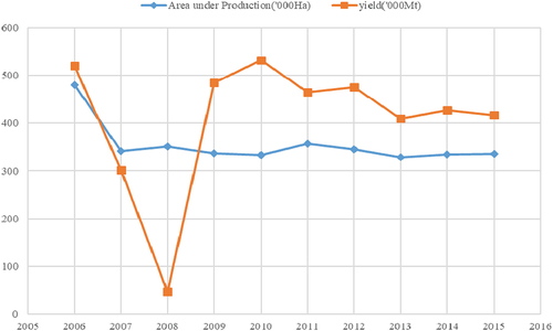
compared to low-income countries. it has been emphasized that the Maputo Declaration serves as a signal for strong political resolution of African leaders to revitalize agriculture as a driver of economic growth, reducing poverty and food and nutrition insecurity (Badiane et al., 2015). These efforts have become necessary because agricultural production and productivity has for the past decades not seen the light of progressive growth rate in Sub-Saharan Africa (SSA; Norton, 2004; Adzawla et al., 2015). In Ghana, the average yield of maize, groundnut, rice and yam, have been estimated as; 1.7Mt/ha, 1.5Mt/ha, 2.4 Mt/ha, and 15.3 Mt/ha, respectively, as against the estimated potential yield of 6.0Mt/ha, 2.5Mt/ha, 6.5 Mt/ha, and 49Mt/ha, respectively (Ministry of Food and Agriculture (MOFA), 2016). Following this, it can be noted that output of groundnut per hectare for the past years had been on the declining rate despite the abundant resources that are needed for its production in Ghana (refer to Figure 1). The trends of groundnut production in Ghana as depicted by Figure 1 also shows that land area cultivated and output obtained are not concurrent.

Figure 1. Trends of groundnut production in Ghana.Source: Authors Own Plot with Data from MoFA 2016

The agriculture’s sector contribution to the gross domestic product of Ghana’s economy cannot be over emphasized as it contributed about 24% on the average (over the last decade) to the annual GDP of Ghana (Budget of Ghana 2010–2020). Out of the five (5) sub-sectors of agriculture in Ghana (crops, livestock, cocoa, forestry and fisheries), the crop sub-sector of which groundnut is part has greater share of agriculture contribution to GDP (Ghana Statistical Service, 2015).

Groundnut (Arachis hypogaea L.) is the most important legume that contributes partly to the agriculture share of Ghana’s GDP (Ministry of Food and Agriculture (MOFA), 2016). Its production is dominant in the northern part of the country. It serves as a source of both livelihood and nutrition to the producers (Danso-Abbeam et al., 2015). Globally, groundnut is reported to be the fourth oil seed crop, third most significant source of vegetable protein after soybean, followed by cotton seed and it is the thirteenth most important food crop (Taphe et al., 2015). In terms of proportion of nutrients, groundnut seeds contain 20% of carbohydrates; 25% of digestible protein and 50% of high-quality edible oil (Girei et al., 2013). The fruits or nuts can be eaten raw, by boiling or roasted. The nuts are ground into paste and is used in diverse ways including; soup preparation, cake (locally called kulikuli), and extracted for oil. The paste (peanut butter) can be eaten with bread. The by-product of groundnut (fodder) serves as feed for livestock and the cake also serves as an important ingredient in animal feed (Tsigbey et al., 2003). From the agronomic point of view, groundnut plant aids in weed control, soil-water conservation and improves organic matter content in the soil and fixes atmospheric nitrogen into the soil.

Estimates of productivity, technical efficiency levels and their determinants are important in making decisions among farmers if productivity is to be improved. This, therefore, has led to a lot of research work on technical efficiency using the classical methods of estimation (e.g., Maximum Likelihood Estimation technique). Meanwhile, it is argued that the classical methods of estimation have some limitations including inability to make probability statements, inability to incorporate non-sample information into analysis, problem of obtaining exact finite-sample results and its asymptotic property nature (Kurkalova & Carriquiry, 2003; Coelli et al., 2005). However, Bayesian estimation approach has been found as appropriate to overcome the limitations of the classical method of estimation (Tonini, 2011). Authors including Koop et al. (1997); Kim & Schmidt (2000); Kurkalova & Carriquiry (2003); Bezemer et al. (2005); Ehlers, 2011) used Bayesian stochastic frontier models in their various work of efficiency studies. In the light of the benefits of the Bayesian estimation method, this study adopts a Bayesian Stochastic Frontier Model to estimate technical efficiency of farmers in Ghana.

2. Materials and methods

2.1. Conceptual framework

Using the parametric approach, the stochastic frontier model as independently and simultaneously proposed by (Aigner et al., 1977; Meeusen & Van den Broeck, 1977), was employed for this study. The concept behind this model is that the determining factors of output variation of a producer can be grouped into two categories, that is, the noise effect and the inefficiency effect.

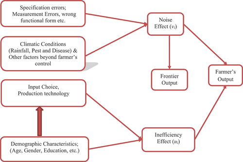
The inefficiency effect consists of the demographic factors and management decisions of the farmer. Figure 2 shows that demographic factors of farmers influence their choice of inputs and technology adopted. These factors are assumed to be controllable by the producer, therefore, any deviation from the frontier output resulting from these factors form the inefficiency on the part of the farmer. The productivity differences of farmers producing under the same noise effect would result from these factors. The noise effect on the other hand, is also due to the specification errors, and climatic conditions. These factors are noted to be beyond the control of the farmer. A positive noise effect (v_i) leads to an increase in the quantity of the output of the deterministic production function. On the other hand, if the effect is negative, there is a reduction in the output of same. (Battese, 1991)

Figure 2. Conceptual framework.Source: Authors own construct, 2022

2.2. Theoretical framework

The theory of production as it relates to efficiency can be traced as far back as Farrel (1957). He defined efficiency as the capacity to produce a given level of output at the minimum cost. In addition, Farrel proposed three measurement categories of efficiency, that is; technical, allocative and economic efficiency. This paper basically considers the measure of technical efficiency. In the same work, Farrel asserted that using the stochastic frontier approach, it is possible to estimate individual firms’ performances and compare it to the optimal performance such that we are able to differentiate firms that are efficient from non-efficient ones, as well as explain the differences in their performances. This approach to analysing technical efficiency have been applied by many researchers in the field of agricultural economics to determine efficiency of farmers (Shamsudeen et al., 2011; Adzawla et al., 2015; Onumah et al., 2018). The general form of the Stochastic Frontier Model (SFM) is specified as Equation 1(1) $Y_i=f(x;\beta ).(v_i-u_i)$(1) ;

(1) $Y_i=f(x;\beta ).(v_i-u_i)$(1)

Where; Y_i = the mean output of farmer i, $f(.)$ is a known function of the firm’s (farm’s) inputs, X = 1, …,N and a vector of parameters, β, to be estimated, v_i is the random component representing errors of measurement and other unforeseen occurrences, finally, the u_i is a non-negative error term that represent the technically inefficiency, that is, the amount by which the firms output falls short in terms of the potential output achievable given the inputs and the technology available. The following assumptions about the random variable v_i and the error term u_i were adopted for this study following (Battesse and Coelli, 1995). v_i ~ N(0, σ²)—v_i is assumed to be independently, identically and normally distributed with mean 0 and a constant variance. The u_i is also assumed to be distributed as a truncation of the normal distribution with mean μ_i and a constant variance; u_i~N(μ_i, σ²). In this case, the inefficiency u_i is explained by some exogenous variables which could be expressed as;

(2) ${\mu }_i=z_i\delta$(2)

Where;

μ_i represents inefficiency effects; Z_i denotes a 1 × n vector of exogenous variables, δ is an n × 1 set of unknown parameters of the inefficiency factors to be estimated. Equation (2)(2) ${\mu }_i=z_i\delta$(2) was adopted for the analysis of the technical inefficiency model. Technical efficiency (TE) is expressed as the ratio of the observed output relative to the output of the frontier production function (Battese, 1991).

(3) $T{E}_i=\frac{Y_i}{Y^{\ast }}=exp(-u)$(3)

Where $Y_i^{\ast }=f(x_i;\beta ).exp(v_i)$ and can be obtained from the Equation 1(1) $Y_i=f(x;\beta ).(v_i-u_i)$(1) by replacing it with Y_i and setting u_i to zero (0), implying that there is no inefficiency effect. That is to say that the deviation of the output of the producer is due to only statistical noise and unforeseen circumstances that are beyond the control of the farmer.

Bayesian SFM was proposed and used by authors including; (Van den Broeck et al., 1994; Koop & Steel, 1995; Osiewalski & Steel, 1998). Bayes’ Theorem states that “the posterior probability density function (pdf) is proportional to the likelihood function times the prior pdf” (Coelli et al., 2005). The theory can be specified mathematically as;

(4) $p(\theta \left|y\right.)\propto L(y\left|\theta \right.)p(\theta )$(4)

Where;

P(θ|y) = the posterior pdf; “α” denotes is proportional to; L(y |θ) = the likelihood function and P(θ) = the prior Pdf. θ in Equation 4(4) $p(\theta \left|y\right.)\propto L(y\left|\theta \right.)p(\theta )$(4) denotes the parameters of the model and this includes; u_i, β, and λ. This paper adopted the exponential model because it has been found to be least sensitive to changes in priors, that is, it is least sensitive to changing the prior information that are to be incorporated into the model (Van den Broeck et al., 1994; Battese, 1991). In Bayesian inference, the following assumptions are made about v_i and u_i, in addition to those that were stated earlier for the MLE (Koop & Steel, 1995).

1. $p(v_i\left|{\sigma }^2\right.)=f(v_i\left|0,{\sigma }^2\right.)$ that is, the independent assumption of the v_i with mean zero and a constant variance.

2. u_i and v_i are independent of each other for all farmers.

3. $p(u_i\left|\lambda \right.)=f(u_i\left|1,\lambda )\right.$, thus, the u_i’s are independent of each other (exponential distribution assumption)

Bayesian stochastic frontier function, is known to be a three-level hierarchical model (Kurkalova & Carriquiry, 2003). In the first level, the logarithms of the output of the farmers in kilograms is modelled as normally distributed random variable with mean equal to a linear combination of logarithms of the production inputs minus the amount of inefficiency u_i and with variance as specified in Equation 5(5) $ln(y_i)={\beta }_0+{\beta }_{1}ln{x}_1+\dots .+{\beta }_{N}ln{x}_N+v_i-u_i$(5) ;

(5) $ln(y_i)={\beta }_0+{\beta }_{1}ln{x}_1+\dots .+{\beta }_{N}ln{x}_N+v_i-u_i$(5)

In the second level, technical inefficiency (u_i) is modelled as the exponential random variables to explain technical inefficiencies among the farmers specified as Equation 6; $u_i{\left|{\delta }_{i}z\right.}_i-Gamma(1,\prod _{j=1}^m{\delta }_j^{z_{ji}})$ (6)

Finally, in the Level three of the hierarchical model, priors for the parameters of the model are specified. The following distributions were specified for the various parameters of the model. Βs ~ N(0, ∞)—the intercept and parameters of the production frontier variables has a multivariate truncated normal distribution with zero (0) mean and an infinite variance to depict a non-informative prior. u_i ~N(μ, λ⁻¹); that is, the inefficiency error term u_i has a truncated normal distribution with constant mean and constant variance. ~Ga (0.1, 0.1); the white noise variance also fellows a gamma distribution with flat priors giving non-informative prior for the white noise variance. λ ~ Ga (φ, φ (lnr*)); that is λ has a Gamma distribution, where r* denotes a prior median efficiency which take the value of 0.8 as adopted from literature (Koop et al., 1997; Kim & Schmidt, 2000; Tonini, 2011).

The conditional posterior distribution for each of the parameters are derived from the joint posterior distribution as specified. (For derivation of these functions see, Jondrow et al., 1982).

(7) $p(u_i\left|y,\beta ,h,,\lambda \right.)=f(u_i\left|x;\beta -y_i\right.-{\left(h\lambda \right)}^{-1},h^{-1})\times I(u_i)$(7)

$u_i$ is a truncated normal distribution, $u_i$$\ge$ 0.

(8) $p(\beta \left|y,h,u,\lambda \right.)=f_N(\beta \left|\stackrel{\wedge }{\beta },h^{-1}{(X^{\prime }X)}^{-1}\times I(\beta )\right.$(8)

$\beta$ is a multivariate normal distribution,$\beta$ $\ge$ 0

(9) $p(h\left|y,\beta ,u,\lambda \right.)=f_G(h\left|I/(y+u\right.-X^{\prime }\beta {)}^{\prime }(y+u-X^{\prime }\beta ),I)$(9)

$h$ has a gamma distribution, $h$ $\ge$ 0

(10) $p({\lambda }^{-1}\left|y,\beta ,u,\lambda \right.)=f_G({\lambda }^{-1}\left|(I+1\right.)/(u^{\prime }j,-ln(r^{\ast })),2(I+1))$(10)

${\lambda }^{-1}$ also have a gamma distribution,${\lambda }^{-1}$ $\ge$ 0

Note: h in the equations = σ² in this paper

The Gibbs sampler was then adopted by the MCMC method to simulate draws for each of the parameters of the model. With the draws, the posterior distributions of the parameters of the model were then approximated and summarized using posterior density functions into descriptive statistics such as the mean, variances and percentiles as presented in the results and discussion section.

2.3. Empirical model specification

Both the Cobb-Douglass and translog functional forms were initially considered for this paper and the latter chosen based on its Deviance Information Criterion (DIC) value. In analysing Bayesian SFM, the DIC value is used to measure the fitness of a model for a particular data and the model with the least DIC value best fit the data (Ehlers, 2011).

Considering the output and input variables of this study, the empirical model for the analysis was specified as;

(11) $lny=ln{\beta }_0+\sum _{i=1}^4{\beta }_{i}ln{x}_i+\frac{1}{2}\sum _{i=1}^4\sum _{j=1}^4{\beta }_{ij}ln{x}_{i}ln{x}_j+(v_i-u_i)$(11)

Where;

Y = Output of groundnut (kg/acre), X₁ = Labour (man-days/acre), X₂ = Seed (kg/acre), X₃ = Herbicides (litres/acre), X₄ = intermediate inputs (GH₵/acre). Note that all variables of Equation 11(11) $lny=ln{\beta }_0+\sum _{i=1}^4{\beta }_{i}ln{x}_i+\frac{1}{2}\sum _{i=1}^4\sum _{j=1}^4{\beta }_{ij}ln{x}_{i}ln{x}_j+(v_i-u_i)$(11) are normalised by their corresponding farm size so that there will be no land size effect on the analysis. The normalisation eliminates farm size as a variable (reduces the number of variables) which is significant in controlling for the occurrence of multicollinearity with translog functional form.

2.3.1. Estimating productivity

The productivity levels of the farmers were analysed by calculating the elasticities and return to scale of the farmers. Since this study employed translog functional form, all variables of Equation 12(12) ${\epsilon }_{{\mathrm{y}}_{\mathrm{i}}}=\frac{\mathrm{\partial }lnE(Y_i)}{\mathrm{\partial }ln{X}_{ji}}=\left\{{\beta }_j\right.+{\beta }_{jj}ln{X}_{ji}+\sum _{i=1}^4{\beta }_{jk}ln\left.X_{ki}\right\}={\beta }_j$(12) were normalised with their respective means to have unit means so that the first order parameter estimates were interpreted as the elasticities. The elasticities are then obtained by taking the derivatives of output variable with respect to the input variables in Equation 11(11) $lny=ln{\beta }_0+\sum _{i=1}^4{\beta }_{i}ln{x}_i+\frac{1}{2}\sum _{i=1}^4\sum _{j=1}^4{\beta }_{ij}ln{x}_{i}ln{x}_j+(v_i-u_i)$(11) as shown in Equation 12(12) ${\epsilon }_{{\mathrm{y}}_{\mathrm{i}}}=\frac{\mathrm{\partial }lnE(Y_i)}{\mathrm{\partial }ln{X}_{ji}}=\left\{{\beta }_j\right.+{\beta }_{jj}ln{X}_{ji}+\sum _{i=1}^4{\beta }_{jk}ln\left.X_{ki}\right\}={\beta }_j$(12) . From Equation 12(12) ${\epsilon }_{{\mathrm{y}}_{\mathrm{i}}}=\frac{\mathrm{\partial }lnE(Y_i)}{\mathrm{\partial }ln{X}_{ji}}=\left\{{\beta }_j\right.+{\beta }_{jj}ln{X}_{ji}+\sum _{i=1}^4{\beta }_{jk}ln\left.X_{ki}\right\}={\beta }_j$(12) , the coefficients of the squared terms and the cross-product terms are equated to zero so that the first terms, β_j’s, are interpreted as direct elasticities.

(12) ${\epsilon }_{{\mathrm{y}}_{\mathrm{i}}}=\frac{\mathrm{\partial }lnE(Y_i)}{\mathrm{\partial }ln{X}_{ji}}=\left\{{\beta }_j\right.+{\beta }_{jj}ln{X}_{ji}+\sum _{i=1}^4{\beta }_{jk}ln\left.X_{ki}\right\}={\beta }_j$(12)

Return to scale (RTS) value of the farmers was computed by the summation of the individual elasticities as;

(13) $RTS=\sum {\epsilon }_{y_i}$(13)

The value of RTS indicates the scale of production of the farmers, such that a value of RTS>1; RTS<1 and RTS = 1 implies increasing return to scale, decreasing return to scale and constant return to scale respectively.

2.3.2. Estimation of technical efficiency

The technical efficiency of the ith farmer is obtained by taking the ratio of the output obtained by the ith farmer (Y_i) relative to the fully efficient output (Y*) as depicted in Equation 3(3) $T{E}_i=\frac{Y_i}{Y^{\ast }}=exp(-u)$(3) .

2.3.3. Explaining technical inefficiency

Following Equation 2(2) ${\mu }_i=z_i\delta$(2) , an empirical model was specified to explain technical inefficiency among groundnut farmers as;

(14) ${\mu }_i={\delta }_0+\sum _{i=1}^5{\delta }_i{z}_i+{\omega }_i$(14)

Where;

δ₀ = constant; δ_i = parameters of inefficiency variables to be estimated; Z_i = inefficiency variables; ω_i = error term to capture the effect of inefficiency variables that are not captured in the model. The error term µ_i is used to explain inefficiency among groundnut producers. The variables in Equation 14(14) ${\mu }_i={\delta }_0+\sum _{i=1}^5{\delta }_i{z}_i+{\omega }_i$(14) are the socio-economic characteristics of the farmers as well as some exogenous factors. Table 1 gives the description, measurement, a priori expected signs and literature that support the choice of variables and their a priori expected signs.

Table 1. Summary of inefficiency variables and a priori expectations

Variable	Description	Measurement	A priori Sign	Literature Support
Z1	Age of farmer	Number of years	+/-	Bezemer et al. (2005)
Z2	Gender of farmer	Dummy (male = 0 & female = 1)	+/-	Bezemer et al. (2005)
Z3	Educational level	Number of years spent in school.	+	Danso-Abbeam et al. (2015)
Z4	Household Size	Number of persons	+	Taphe et al. (2015)
Z5	Extension visits	Frequency of times	+	Mahgoup et al. (2017)

Source: Field Survey, 2017

2.4. Study area and sampling procedure

Three administrative regions of Ghana including; Oti, Northern and Upper West regions were purposively selected for the study. The choice of the regions was based on the fact that groundnut is produced in large quantities in those regions and they best serve as a representative (Martey et al., 2015). In each of the three regions, two districts each were also purposively chosen from each of the three regions on the basis of their records in groundnut production. These includes; Krachi Nchumuru and Krachi West from Oti region, Nanumba South and Yendi Municipality from Northern region and Sissala West and Sissala East from Upper West Region. Subsequently, two communities from each district, were randomly selected from the six district which made up a total of 12 communities. Finally, twenty-five (25) farmers were randomly selected from each of the communities and interviewed with a well-designed questionnaire amounting to a sample size of 300 farmers.

3. Results and discussions

3.1. Productivity levels of groundnut producers

Result from the analysis revealed that average output of groundnut is 326.33 kg with a range of 20 kg (min) to 2,722.50 kg (max). Meanwhile, in terms of per acre basis, the minimum and maximum output of groundnut were found to be 9.33 kg and 595 kg respectively. Mean output per acre was also noted to be 134.74 kg. Comparatively, this output value (converting 134.74 kg/ha to Mt/ha gives a value of 0.34mt/ha) is far less than that of the national output of 1.65mt/ha (Ministry of Food and Agriculture (MOFA), 2016). The estimates from the translog model indicate that a percentage increase in any of the inputs lead to an increase in the productivity level of groundnut (Table 2). This implies that the production function is well behaved and satisfies the monotonicity assumption as noted by (Tonini, 2011). This means that farmers could continue to increase their input levels to the point that any increase in the input level would yield no additional output (constant return to scale). The sum of elasticities of the estimated translog model gives RTS value of 1.10 which means that the production function of the groundnut farmers demonstrates an increasing return to scale. This indicates that when all inputs are increased by 1%, groundnut output in the study area will increase by 1.10%. The return to scale value in this study is different from that obtained by (Shamsudeen et al., 2011), who found groundnut producers in West Manprusi district of northern Ghana to be producing at a constant return to scale—RTS value of 1.03. Following the work of (Danso-Abbeam et al., 2015), who employed the translog functional form, the estimates of the first order coefficient showed that farmers were producing at an increasing return to scale.

Table 2. Bayesian Parameter Estimates of the Stochastic Frontier Model

Variable	Parameters	Mean	SD	MC_err	2.5%	Median	97.5%
Constant	β0	0.326	0.124	0.006	−0.020	0.348	0.507
Labour	β1	0.269	0.112	0.002	0.054	0.264	0.498
Seed	β2	0.547	0.131	0.002	0.290	0.547	0.806
Herbicides	β3	0.215	0.084	0.009	0.048	0.215	0.379
Intermediate Input	β4	0.071	0.126	0.002	−0.183	0.072	0.317
Labour Square	β5	−0.566	0.339	0.004	−1.208	−0.573	0.097
Seed Square	β6	−0.658	0.273	0.003	−1.190	−0.660	−0.118
Herbicide Square	β7	−0.166	0.185	0.002	−0.529	−0.165	0.198
Intermediate Input Square	β8	−0.167	0.151	0.002	−0.461	−0.168	0.131
Labour * Seed	β9	1.000	0.221	0.003	0.565	1.001	1.426
Labour * Herbicides	β10	−0.804	0.165	0.002	−1.132	−0.802	−0.481
Labour * Intermediate Inputs	β11	−0.082	0.170	0.002	−0.408	−0.083	0.255
Seed * Herbicides	β12	0.472	0.184	0.003	0.113	0.475	0.826
Seed * intermediate Inputs	β13	0.084	0.169	0.002	−0.247	0.083	0.421
Herbicide* Intermediate inputs	β14	0.044	0.087	0.001	−0.121	0.043	0.212
White-noise variance	σ^2	0.223	0.066	0.003	0.141	0.043	0.405
Lambda	λ	0.295	0.098	0.004	0.007	0.298	0.567
DIC		521.50

Source: Field survey with Authors Own Calculations

3.2. Posterior distributions of the parameters of the stochastic frontier model

Table 2 presents the posterior distributions of the parameter estimates. The Gibbs sampler was run for one chain, with burn-in of 20,000 iterations, 80,002 retained draws and a thinning to every 20th draw in order to reduce the level of autocorrelation of the chain. One way to check the accuracy of the estimates in Table 2, is by comparing the Monte Carlo (MC) error with the corresponding posterior standard deviation. Convergence is normally achieved when the MC errors are found to be lower than the standard deviation (Tonini, 2011). From Table 2, it can be realized that the MC error values are lesser than their corresponding standard deviation values, indicating the convergence of the estimated model and accuracy of the estimates.

Sigma square value (σ²), the variance of the white noise in Table 2 explains the variation of total output due to random factors (Kurkalova & Carriquiry, 2003). The value of the sigma square was found to be 0.223. This means that 22.3% of the variation in total output is due to random shocks. In other words, it can be deduced that 77.7% of the variation in total output is associated to farmer specific factors.

The value of lambda—λ, gives information about the inefficiency level of the farmers. In other words, it shows by how much the producer has fallen short of the total output. The value of λ (0.295) in Table 2 denotes that the groundnut farmers are 29.5% technically inefficient. That is to say that the groundnut farmers are producing at 70.5% of the total groundnut output that can be obtained given the input resources and the technology at hand.

The estimates of the production elasticities (at the sample mean) for labour, seed, herbicide, and intermediate inputs are; 0.269, 0.547, 0.2145 and 0.071 respectively. All the input variables met their a priori expectation. The result of the parameter estimates implies that a percentage increase in labour, seed, herbicides and expenditure on intermediate inputs will lead to a corresponding increase of 0.27%, 0.55%, 0.21% and 0.07% into total output of groundnut respectively.

SD = Standard Deviation; MC_err. = Monte Carlo error; DIC: Deviance Information Criterion; % = Percentile

From the result of the input elasticities, it has been demonstrated that seed contributes largely to increase in output level compared to the other input variables in the model. This result commensurate the work of (Taphe et al., 2015) who found groundnut seed as the most important input factor among the other input variables that increases output of groundnut in Taraba State in Nigeria. The study of (Shamsudeen et al., 2011) also noted a positive relationship between output of groundnut and seed sown.

The positive relationship between labour and groundnut output is also in agreement with the work of (Danso-Abbeam et al., 2015). Asekenye (2012) also found a positive relationship between output of groundnut and labour among groundnut farmers in Kenya. However, he noted a positive statistically insignificant effect for this variable among the groundnut farmers in Uganda in same study. Shamsudeen et al. (2011) on the contrary found a negative insignificant relationship between output of groundnut and labour. The possible implication of this relationship between output of groundnut and labour in this current study is that as labour used per acre increases, cultural activities performed are done with accuracy.

Herbicide usage was found to have a positive effect on groundnut output, thus, increase in the quantity of herbicide lead to increase groundnut output. This finding commensurate the work of (Taphe et al., 2015) who noted a positive relationship between output of groundnut and agrochemicals among small scale farmers in Taraba State of Nigeria. Farmers who used herbicide during land preparation stage opined that as the weeds are controlled with the herbicide before sowing of the groundnut, the growth of weeds in the field is suppressed and the groundnut turn to grow faster.

The positive relationship between output of groundnut and intermediate inputs implies that as the amount of money spent on intermediate inputs increases, output level of groundnut increases. This could be explained in diverse ways, for example, increased output would mean increased in the quantity of sacks needed to store groundnut and for that matter increased expenditure on sacks. From Table 2, all the squared terms of the input variables have a negative sign as opposed to the positive sign observed for the first order parameters of the input variables. The implication is that output will increase initially when input levels are increased, but as more and more of the inputs are added, output level eventually reduces at the long run

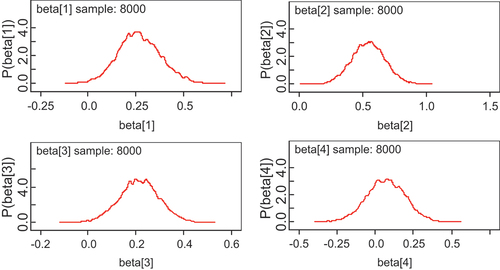
The Bayesian approach, unlike the frequentist approach, allows the posterior kernel density to be recovered for all parameter estimates instead of a single point estimate. This gives more information about the underlying parameter certainty (Tonini, 2011). Figure 3 shows the posterior kernel density for the first order parameter estimates of the model.

Figure 3. Posterior kernel density plots of input variable parameters.

3.3. Technical efficiency levels of groundnut farmers in Ghana

Bayesian econometrics provides additional information about farmers’ technical efficiency scores that are not provided in the classical methods (Griffin & Steel, 2007).

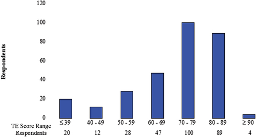
The minimum and maximum technical efficiency scores were found to be 13% and 95.1% respectively, with an average of 70.5%. The technical efficiency scores imply that given the inputs and the technology adopted by the farmers, the least efficient farmer was producing at 13% of the output of groundnut, whiles the most efficient groundnut farmer among the respondents produces at 95.13% of the total output obtainable. The predicted average technical efficiency score implies that on the average, groundnut farmers interviewed are producing at 70.5% of the total output of groundnut achievable, given the inputs and the technology adopted. Figure 4 shows the technical efficiency scores across the respondents. This result is different from the work of (Taphe et al., 2015) who found the mean technical efficiency score of groundnut farmers to be 77%.

Figure 4. Distribution of Technical Efficiency Scores of Farmers.Source: Field Survey with Author’s Own Plot

The implication of the technical efficiency value of 70.5% is that on average, there is an output loss of 29.5% resulting from inefficiency. From the estimate of the white noise variance, it implies that 22.3% of the 29.5% output loss is due to factors that are beyond the control of the farmer. Therefore, controlling for about 77.7% of the 29.5% loss of output would reduce output loss to about 9.5%.

3.4. Determinants of inefficiency of groundnut farmers

Table 3 presents the posterior distribution of the inefficiency variables. The value of parameters (δs) of the inefficiency variables that are essentially different from one indicates the ability of the corresponding exogenous factor to explain technical inefficiency (Kurkalova & Carriquiry, 2003). Specifically, value of parameters greater than one implies that the corresponding inefficiency variable has a negative effect on technical inefficiency. From Table 3, the parameter value of variables including; gender of farmers, educational level of farmers and number of extension visits are significantly greater than 1 indicating their explanatory power on technical inefficiency. These variables met their a priori expectation sign.

Table 3. Posterior Distributions of Determinants of Inefficiency

Variables	Param-eters	Mean	SD	MC_error	2.5%	Median	97.5%
Constant	δ0	1.504	0.466	0.997	0.654	1.460	2.819
Age of famer	δ1	0.899	0.771	0.001	0.045	0.201	2.483
Gender of farmer	δ2	1.743	1.079	0.002	0.078	0.185	5.929
Educational level	δ3	2.309	1.599	0.030	0.115	0.294	7.991
Household size	δ4	0.872	0.617	0.002	0.044	0.128	2.877
Extension visits	δ5	1.413	1.046	0.011	0.053	0.367	5.100

Source: Field Survey with Author’s Own Calculations

The value of parameter estimate of the variable gender implies that female groundnut farmers are less technically inefficient than their male counterparts. This higher efficiency level of female groundnut farmers may be due to the fact that they are committed to their groundnut farms and perform their cultural practices on timely basis. Martey et al. (2015) noted that groundnut production is a female dominated economic activity in northern Ghana. Most males who engaged in groundnut production do it as an extra farm activity and do not regard it as a major farm economic activity

Educational level also had a value of 2.3 which is significantly above 1 and implied a negative effect on technical inefficiency. The negative effect of education on technical inefficiency means that as the educational level of the farmer increases, their inefficiency level also reduces. The result on education is in agreement with the work of (Mahgoup et al., 2017), who found a negative relationship between technical inefficiency and years of education in Sudan. They argued that the negative relationship between technical inefficiency and years of education demonstrates the potentials of groundnut farmers who attained formal education to adopt new agricultural technologies, understand and implement agricultural extension recommendations and efficiently allocate their resources to increase their productivity levels.

Extension visits parameter also had a value of 1.4 which is above 1, indicating a negative relationship between numbers of extension visits the farmer had within the production season and their technical inefficiency levels. In other words, farmers who were visited frequently by agricultural extension agents were found to be less technical inefficient compared to their counterpart farmers who received less or no visit. The result is in conformity with the work of (Taphe et al., 2015) who noted a negative relationship between technical inefficiency and extension visit. This relationship is suggested to be due to the fact that farmers who had access to extension contact are likely to become aware and could adopt new agricultural technologies and improve upon their cultural practices in the farm. Recommendations made by extension workers are expected to enhance farm management level decisions of the farmer. Farm management level decisions have a great impact on farmers’ level of efficiency.

The other inefficiency variables had parameter values below 1 and implied lack of statistical explanatory power. The lack of explanatory power by these variables is common in Bayesian technical efficiency analysis (Bezemer et al., 2005).

5. Conclusions and recommendations

5.1. Conclusion

This paper estimated the productivity and technical efficiency levels of groundnut farmers in Ghana and as well determined the factors that explain the technical inefficiency using Bayesian SFM. Bayesian approach was adopted because, it was possible to derive a full posterior distribution of any individual efficiency, impose regularity conditions on the parameters that would be estimated through consistently specification of the priors and considered parameter uncertainty by providing probability distribution for each estimated parameter. A total sample of 300 groundnut farmers were interviewed.

This study concludes that groundnut farmers are producing at the stage one of the production function. Producing at the stage one is not economically viable, since increasing inputs leads to increasing output, and the implied need for improvement at this stage.

The predicted technical efficiency scores implied that on the average groundnut producers in Ghana are producing at a technical efficiency level of 70.5% and none of the producers were found to be fully efficient.

From the inefficiency model analysis, it has also been concluded that factors including; gender of the farmers, extension visit to farmers and educational levels of the farmers, significantly explain inefficiencies among the farmers interviewed.

5.2. Policy recommendations

The study recommends increased scale of production with effective management decisions by groundnut farmers so as to take advantage of economies of scale of production since farmers were found to be producing at an increasing return to scale.

The study also recommends that groundnut farmers should be given the necessary support in the form of subsidy on inputs including; groundnut seeds, herbicides and intermediate inputs by the district assemblies through the department of agriculture to enable them fill the gap in output so as to increase the level of technical efficiency as they only produce at efficiency score of 70.5%.

The study also strongly recommends that government through MoFA should extend the scope of extension delivery and increase the number of extension agents. Increase in the scope of extension delivery because most areas were found not to be part of the catchment areas of the extension agents and farmers in those areas did not receive any extension visit. Furthermore, when the number of extension agents is increased, it will improve upon farmer/AEA ratio and subsequently increase the number of visits. District assemblies through department of agriculture should facilitate access to information to farmers who did not have access to formal education. These farmers should also be given intensive training to boost their level of understanding of recommendations and new technologies introduced to them.

Acknowledgement

The authors declare that this research has not receive any funding for the executing of the work nor has it receive any funding for the publication cost.

Disclosure statement

No potential conflict of interest was reported by the author(s).

Additional information

Funding

The authors received no direct funding for this research.

Notes on contributors

Dominic Chakuri

Dominic Chakuri is a PhD student at the Department of Agricultural Economics and Agribusiness, University of Ghana, Legon, Accra. His research interest includes productivity and efficiency analysis, poverty analysis, and environmental sustainability.

Freda Elikplim Asem

Freda Elikplim Asem is a lecturer at the Department of Agricultural Economics and Agribusiness, University of Ghana. She holds a PhD in Development Studies, from the University of Ghana. She is passionate about agriculture development in Ghana and Africa at large, particularly in relation to small holder farmer. Her research interests include agricultural marketing, agribusiness, agrifood systems and agricultural value chains analysis.

Edward Ebo Onumah

Edward Ebo Onumah is a Senior lecturer at the Department of Agricultural Economics and Agribusiness, University of Ghana. He holds a PhD in Agricultural Sciences with a specialty in Agricultural Economics from Georg-August University of Göttingen, Germany. His research interest includes productivity and efficiency analysis, agricultural production risk and uncertainty, food security investigation, microfinance and poverty analysis, economics of aquaculture and fisheries investigation, and agricultural trade and market analysis.

References

- Adzawla, W., Donkoh, S. A., Nyarko, G., O’reilly, O. O. E., & Awai, P. E. (2015). Technical efficiency of bambara groundnut production in Northern Ghana, 2(2). UDS International Journal of Development. UDSIJD. http://www.udsijd.org
- Aigner, D. J., Lovell, C. A. K., & Schmidt, P. (1977). Formulation and estimation of stochastic frontier production function models. Journal of Econometrics, 6(1), 21–15. https://doi.org/10.1016/0304-4076(77)90052-5
- Alexandratos, N., & Bruinsma, J. (2012). World Agriculture Towards 2030/2050, the 2012 revision. Agriculture Development Economics Division, 12(03), 15–160. www.fao.org/fileadmin/templates/esa/Global_persepctives/world_ag_2030_50_2012_rev.pdf
- Asekenye, C., (2012). An Analysis of Productivity Gaps among Smallholder Groundnut Farmers in Uganda and Kenya. Master’s thesis. Master’s thesis: University of Connecticut Graduate School at DigitalCommons@UConn. http://digitalcommons.uconn.edu/gstheses/323
- Badiane, O., Makombe, T., Lam, E., Nicholson, J., Oumar Ba, I., Diallo, A., Fall, A., Masresha, B. G., & Goodson, J. L. (2015). Beyond a middle income Africa: Transforming african economies for sustained growth with rising employment and incomes. ReSAKSS Annual Trends and Outlook Report 2014. Washington, D.C.: International Food Policy Research Institute (IFPRI). 36(9), 1708–1717. https://doi.org/10.1111/risa.12431.
- Battese, E. G. (1991). Frontier production functions and technical efficiency: A survey of empirical applications in agricultural economics. Agricultural Economics, 7(3–4), 185–208. https://doi.org/10.1016/0169-5150(92)90049-5
- Bezemer, D., Balcombe, K., Davis, J., & Frazer, I. (2005). Livelihood and Farm Efficiency in Rural Georgia. Applied Economics. University of Groningen. https://doi.org/10.1080/00036840500215253.
- Coelli, T. J. (1995). Recent development in frontier modelling and efficiency measurement. Australian Journal of Agricultural Economics, 39(3), 219–245. https://doi.org/10.1111/j.1467-8489.1995.tb00552.x
- Coelli, T., Rao, D. S. P., O‟Donnell, C. J., & Battese, G. E. (2005). An Introduction to Efficiency and Productivity Analysis. Springer Publication.
- Danso-Abbeam, G., Dahamani, A. M., & Bawa, A.-S. (2015). Resource-use- efficiency among mallholder groundnut farmers in Northern Region, Ghana. American Journal of Experimental Agriculture, 6(5), 290–304. https://doi.org/10.9734/AJEA/2015/14924
- Ehlers, S. R. (2011). Comparison of Bayesian models for production efficiency. In Journal of Applied Statistics (Vol. 38. pp. 2433–2443). Taylor & Francis Group. https://doi.org/10.1080/02664763.2011.559203
- Farrel, M. J. (1957). The measurement of productive efficiency. Journal of Royal Statistical Society, 3(3), 253–290. https://doi.org/10.2307/2343100
- Ghana Statistical Service. (2015). Annual Gross Domestic Product. Statistics for Development and Progress. Ghana statistical service.
- Girei, A. A., Duana, Y., & Dire, B. (2013). An economic analysis of groundnut (Arachis hypogea) production in Hong Local Government Area of Adamawa State, Nigeria. Journal of Agricultural and Crop Research, 1(6), 84–89.
- Griffin, E. J., & Steel, J. F. M. (2007). Bayesian stochastic frontier analysis using WinBUGS. In Journal of Productivity Analysis (Vol. 27pp. 163–176.). Springer. URL. http://www.jstor.org/stable/41770273
- Jondrow, J., Lovell, V. A. K., Materov, I. S., & Schmidt, P. (1982). On the estimation of technical efficiency in the stochastic frontier production function model. Journal of Econometrics, 19(2–3), 233–238. https://doi.org/10.1016/0304-4076(82)90004-5
- Kim, Y., & Schmidt, P. (2000). A review and empirical comparison of bayesian and classical approaches to inference on efficiency levels in stochastic frontier models with panel data. Journal of Productivity Analysis, 14(2), 91–118. https://doi.org/10.1023/A:1007801006988
- Koop, G. J., Osiewalski, Steel, M. F. J., & J, S. M. F. (1997). Bayesian efficiency analysis effects: Hospital cost frontiers. Journal of Econometrics, 76(1–2), 77–105. https://doi.org/10.1016/0304-4076(95)01783-6
- Koop, G. J., & Steel, M. F. J. (1995). Bayesian analysis of Stochastic frontier models. University of Edinbergh.
- Kurkalova, L. A., & Carriquiry, A. (2003). Input- and output-oriented technical efficiency of Ukrainian collective farms, 1989-1992: Bayesian analysis of a stochastic production frontier model. Journal of Productivity Analysis, 20(2), 191–211. Springer. https://doi.org/10.1023/A:1025132322762
- Mahgoup, O. B., Ali, A. E. S., & Mirghani, A. O. (2017). Technical efficiency analysis of groundnut production in the gezira scheme, Sudan. International Journal of Scientific and Research Publications, 7(1). www.ijsrp.org
- Martey, E., Wiredu, N. A., & Oteng-Frimpong, R. (2015). Base line study of groundnut in northern Ghana. Lambert Academic Publishing.
- Meeusen, W., & Van den Broeck, J. (1977). Efficiency estimation from cobb- douglas production functions with composed errors. International Economic Review, 18(2), 435. https://doi.org/10.2307/2525757
- Ministry of Food and Agriculture (MOFA). (2016). Agriculture in Ghana: Facts and Figures (2015). Statistics, Research and Information Directorate (SRID), Ministry of Food and Agriculture, Ghana.
- Norton, R. D. (2004). Agricultural development policy: Concepts and experiences. John Wiley & sons, Ltd, The Atrium.
- Onumah, E. E., Onumah, A. J., & Onumah, G. E. (2018). Production risk and technical efficiency of fish farms in Ghana. Science Direct, 05.033(495), 55–56. https://doi.org/10.1016/j.aquaculture
- Osiewalski, J., & Steel, M. F. J. (1998). Numerical tools for the Bayesian analysis of stochastic frontier models. Journal of Productivity Analysis, 10(1), 103–117. https://doi.org/10.1023/A:1018302600587
- Shamsudeen, A., Donkoh, S. A., & Sienso, G. (2011). Technical efficiency of groundnut production in West Mamprusi District of Northern Ghana. Journal of Agriculture and Biological Sciences, 2(4), 71–77. http://www.globalresearchjournals.org/journal/?a=journal&id=jabs
- Taphe, B. G., Agbo, F. U., & Okorji, E. C. (2015). Resource productivity and technical efficiency of small scale groundnut farmers in Taraba State, Nigeria. Journal of Biology, Agriculture and Healthcare, 5(17), 2224–3208. www.iiste.org
- Tonini, A. (2011). Bayesian stochastic frontier: An application to agricultural productivity growth in European countries. In Economic Change and Restructuring (Vol. 45, pp. 247–269). Springerlink.com. Springer, US.
- Tsigbey, F. K., Brandenburg, R. I., & Clottey, V. A. (2003). Peanut production methods in northern ghana and some disease perspectives. Online Journal of Agronomy, 34, 36–47.
- Van den Broeck, J., Koop, G., Osiewalski, Steel, M. F. J., & Osiewalski, J. (1994). Stochastic frontier models: A bayesian perspective. Journal of Econometrics, 61(2), 273–303. XXXV-1:48–6. https://doi.org/10.1016/0304-4076(94)90087-6.