Time-frequency moment interdependence of equity, oil, and gold markets during the COVID-19 pandemic

Abstract

Like no other calamitous event in recent memory, the COVID-19 pandemic has plunged the world’s financial system into disarray, triggering systemic risk spillovers across markets. In this study, we use 5-minute index futures price data to examine the multiscale interdependence structure of global equity, gold, and oil markets prior to and following the COVID-19 outbreak, in terms of the first four realized moments of their respective return distributions (i.e., mean, variance, skewness, and kurtosis). With respect to the equity-gold nexus, we find that stock (gold) returns and volatility negatively (positively) lead their gold (stock) counterparts at medium- and long-term scales in the pandemic period, while asymmetry risk in stock markets positively leads its counterpart in gold markets at the same scales before and during the early months of the health crisis. Concerning the oil-equity nexus, our results reveal a positive (negative) co-movement between asymmetry risks at short- and medium-term scales in January-April (May-July) 2020, whereas heavy tail risks are positively synchronized at low frequencies in the turbulent period of March-April 2020. Some policy implications are derived from the analysis.

Keywords:

• Equity markets
• gold
• crude oil
• realized moments
• moment linkage
• wavelet phase-difference

JEL classification:

• C32
• C53
• G10

PUBLIC INTEREST STATEMENT

This study conducts a three-dimensional wavelet analysis to examine the multiscale co-movement dynamics and lead-lag effects of the world’s equity, gold, and oil markets prior to and in the aftermath of the COVID-19 outbreak, in terms of the first four moments of their respective return distributions (i.e., mean, variance, skewness, and kurtosis). The results show that stock-gold and oil-stock market pairs are linked not only through mean and volatility, but also through skewness and, sometimes, kurtosis, which imply that patterns of asymmetry and tail dependence should be considered when it comes to building cross-asset class portfolios. Besides, gold still stands out as a battle-tested and recession-proof investment alternative.

1. Introduction

In a world of apparently ever-escalating uncertainty, large-scale crises, whether of a political, economic, social, or public-health nature, continue to be an overriding prognostic and causal risk factor to the global system. The spiraling spatio-temporal spread of the novel coronavirus (2019-nCoV) is one such example, potentially bringing economic and financial Armageddon to the world. With, perhaps, no end in sight to its calamities, the COVID-19 pandemic has disrupted both people’s livelihoods and businesses of all sizes across industries. Many corporate giants, especially in energy, transportation, and tourism sectors, have been on the edge of a financial precipice, while others have taken drastic actions to ensure their survival. Governments have introduced different measures to maintain an optimal balance between saving lives and weathering the pandemic’s socioeconomic repercussions. To control the disease’s further propagation, many countries have adopted strict lockdowns and other temporary mitigation and containment strategies, which, in turn, weighed heavily on supply and demand sides. Baker et al. (2020) indicate that the present emergency gives rise to a profound degree of uncertainty, which exceeds the one accompanied the 2007–2009 global financial crisis and is comparable in magnitude to the uncertainty during the 1929–1933 Great Depression. Yarovaya et al. (2022) highlight that the pervasive uncertainty surrounding the pandemic has sent the world economy into a tailspin.

As forward-looking indicators of future economic circumstances, financial markets have not been far afield from the shocks emanating from the COVID-19 crisis. Since its outbreak in the early weeks of 2020, the virus has wreaked havoc on advanced and emerging equity markets alike, leading to abrupt shifts in market-wide investor sentiment. With much pessimism regarding the pandemic’s trajectory spooking investors into a panic sell-off, the world’s major equity indices have experienced a dramatic collapse. Over the course of four weeks in February and March, benchmark indices racked up losses of more than $16 trillion. For instance, the US S&P 500, Europe’s EURO STOXX 600, London’s FTSE 100, Japan’s Nikkei 225, Australia’s S&P/ASX 200, Hong Kong’s Hang Seng, Thailand’s SET 100, and South Korea’s KOSPI indices posted massive falls, shedding between 10% and 40% of their respective values. Level 1 market-wide circuit breakers (MWCB) for the US stock markets halted trading on multiple occasions on 9 March 2012, 16, and 18, in view of steep price declines (World Economic Forum, 2020).¹ Since its institution in 1988, the MWCB has kicked in only once during the 1997 Asian financial crisis. Albuquerque et al. (2020) contend that the COVID-19 outbreak and its ensuing systemic effects are thought to be an extraordinary exogenous shock to global equity markets. Dai et al. (2021) demonstrate that the severity of the pandemic tends to amplify the crash risk (measured by the conditional skewness) of the US stock market.

In parallel, the health crisis has not left crude oil markets unscathed. Due to the subsequent confinement measures enforced worldwide (e.g., border closures, business lockdowns, mobility restrictions, shutdown of entertainment destinations, flight suspension), global demand for black gold cratered. The July 2020 oil market report, by the International Energy Agency (IEA), indicates that the world petroleum demand declined by 16.4 million barrels a day (mb/d) year-on-year in the second quarter of 2020, and it is expected to shrink by 7.9 mb/d in the same year and to rebound in growth by 5.3 mb/d in 2021. Over the January-March 2020 quarter, China, the first country plagued by the virus and the world’s foremost importer of oil and liquefied natural gas, reduced considerably demand for energy products, because of the pandemic-driven business disruptions. On the supply side, amid an unprecedented oil glut, energy markets have been battered by a historic price meltdown due to a fierce price war between Saudi Arabia and Russia, the second- and third-largest suppliers of oil across the globe. Altogether, these influences seem to have contributed to plunging oil prices into an 18-year trough, from which is it is unlikely to bounce back in the near-future term. For example, the spot prices of the European Brent crude and the US West Texas Intermediate (WTI) crude, the world’s primary oil benchmarks, plummeted to record-low levels, where the former dipped by about 83% between March and April, while the latter nosedived far below zero on April 20. Shaikh and Huynh (2022) show that negative news about the COVID-19 pandemic has important explanatory power for global stock, commodity, and foreign exchange markets.

The resultant downside risk in equity and oil markets has created an acute risk-off sentiment, which, in turn, pushed investors towards a flight to safety by resorting to such potential safe-haven candidates as gold. In its gold mid-year outlook 2020 report, the World Gold Council (WGC) highlights that the yellow metal has been the top performing investment in the first half of 2020, ahead of mainstream asset classes with positive year-to-date (YTD) returns of 17%. Besides, by the end of June 2020, holdings of physically-backed gold exchange traded funds (ETFs) hit an all-time high of 3619 tonnes, bringing global net inflows to 732 tonnes, equivalent to $39.4 billion of assets under management. The report emphasizes that the ultra-low interest rate climate and bleak global economic prospects corroborate the typical role of gold as the safe asset of choice. Ji et al. (2020) find that major stock market indices of the US, Europe, and China and the WTI crude oil experience notable changes in the left tail of their respective return distributions in March 2020. The results also suggest gold and soybean commodity futures as effective safe-haven assets during the COVID-19 crisis. Beckmann et al. (2015) demonstrate the relevance of gold as a diversifier and a safe-haven investment in times of extreme market conditions. Kinateder et al. (2021) show that gold acts as a reliable safe-haven investment option during both the global financial turmoil of 2007–2009 and the ongoing COVID-19 pandemic.

The heavy toll that the COVID-19 outbreak has taken on equity and oil markets offers a vivid example of “Black Swan” events or “worst-case” episodes, which are far beyond the scope of common experience and produce enormous losses. Those rare unexpected shocks underline the pertinence of heavy tails to such themes as extreme event dependence, cross-market spillovers, risk management systems, and economic evaluation. Corbet et al. (2021) indicate that the speed and magnitude of the pandemic outbreak epitomize the unique attributes of black swan events. In this respect, it is well acknowledged in the literature that extreme-tail risk events cannot be captured via a Gaussian distribution (e.g., Arditti, 1967; Cont, 2001; Dittmar, 2002; Peiró, 1999; Press, 1967; Sortino & van der Meer, 1991). Lucas and Klaassen (1998) point out that a shortcoming of the normal distribution is that its tails decay exponentially fast to zero and, hence, extreme realizations are indeed unlikely. However, in practice, extremely large returns of either sign, reflecting asset price booms and crashes, occur much more frequently than suggested by the Gaussian distribution. Rubinstein (1973) argues that if returns are not normally distributed and investors’ utility function is non-quadratic, then investors will be concerned not only with the mean and variance, but with higher-order moments as well (i.e., skewness and kurtosis). A strand of research (e.g., Arditti & Levy, 1975; Kraus & Litzenberger, 1976; Scott & Horvath, 1980; Simkowitz & Beedles, 1978) shows that higher-order moment risks matter for explaining returns of risky assets. A preference for positive skewness is an indication of investors’ predilection for lottery-like securities (Bordalo et al., 2012), while negative skewness reflects a source of tail risk (Bollerslev et al., 2015) or crash risk (Kozhan et al., 2012). A leptokurtic (platykurtic) distribution implies that more extreme outcomes are more (less) likely to happen. Since extreme price movements in one market are highly likely to spill over into other markets, it is of great importance to look into the risk transmission mechanisms of extreme returns not only in the context of variance, but also in terms of skewness and kurtosis of empirical distributions. Skewness transmission reveals information about how upside or downside risk spreads across markets, while kurtosis transmission provides vital clues on whether, and to what extent, extreme events propagate across markets. Hou and Li (2020) emphasize that an investigation of the transmission of higher-order moment risks sheds light on informational efficiency and informational linkages in times of wild price swings, which, in turn, may yield crucial implications for the development of appropriate hedging strategies, risk management practices, and optimal portfolio structures. This may also help regulators establish suitable institutional frameworks to curb the cross-market impact of volatility, asymmetry, and heavy tail risks.

Against this backdrop, the current study conducts a three-dimensional wavelet analysis to examine the multiscale co-movement dynamics and lead-lag effects of the world’s equity, gold, and oil markets prior to and in the aftermath of the COVID-19 outbreak, in terms of the first four moments of their respective return distributions (i.e., mean, variance, skewness, and kurtosis). More explicitly, using the wavelet coherence and wavelet phase-difference, we seek concrete answers to the following questions:

1.   What does the time-frequency interdependence structure of global stock and gold markets, in terms of mean, variance, skewness, and kurtosis of their respective return distributions, look like on the heels of the COVID-19 pandemic?

2.   What does the time-frequency interdependence structure of global stock and oil markets, in terms of mean, variance, skewness, and kurtosis of their respective return distributions, look like on the heels of the COVID-19 pandemic?

We contribute to the expanding body of literature on market interdependence in at least three ways. First, although the COVID-19 outbreak has inspired a burgeoning research field that considers the pandemic-induced linkage patterns and contagion effects between financial markets (e.g., Atif et al., 2022; Corbet et al., 2021; Dutta et al., 2020; Elgammal et al., 2021; Ji et al., 2020; Jiang et al., 2022; Kliber & Łęt, 2022; Salisu et al., 2020; Sharif et al., 2020; Sharma et al., 2022), the main contribution of these works revolves around understanding the dynamics of return and/or volatility spillovers, hence overlooking the potential role of downside risk and tail risk dependence in chaotic times. Do et al. (2016) indicate that in view of the recent waves of global financial instability, there is a strong case for a thorough assessment of the propagation of cross-market higher-order moment risks to account for correlated shocks and to predict probable financial crashes. Del Brio et al. (2017) assert that given the cross-country knock-on effects of episodic financial turmoil, a meticulous analysis of market interdependence, with respect to extreme downside risk and tail risk, becomes all the more pertinent. We are unaware of any papers exploring cross-market information transmission, via moments beyond the second order of the return distribution, under the economic and financial pressures of the COVID-19 infection. Our work constitutes one such effort to address this void in the literature.

Second, there are some research attempts (e.g., Del Brio et al., 2017; Do et al., 2016; Finta & Aboura, 2020; Greenwood-Nimmo et al., 2016; Hashmi & Tay, 2007; Hou & Li, 2020) that look into how downside and heavy tail risks are transmitted within and across markets. Nonetheless, these studies draw inferences solely from the time-domain perspective, thus, neglecting information hidden in the frequency domain. That is, they fail to capture the frequency-varying characteristics of higher-order moment spillovers. Thanks to wavelet multiscaling techniques, we are better able to extract information simultaneously from time and frequency spheres. The results of this integrated investigation are expected to elucidate how volatility, asymmetry, and heavy tail risks spread across markets over different time horizons.

Third, even though it is still too premature, at the time of writing, to conduct a comprehensive evaluation of the ripple effects of the ongoing COVID-19 pandemic on financial market dynamics, we endeavor to provide a preliminary assessment of whether cross-market spillovers, in terms of the first four moments, changed in the wake of the outbreak of COVID-19. From a practical standpoint, our evidence generates insights that could be of use to investors and fund managers in such areas as asset price models, portfolio diversification decisions, hedging strategies, and risk management. The implications may also prove beneficial for relevant regulatory authorities charged with minimizing financial stability risks and vulnerabilities.

It should be noted that although the issues addressed in this paper are altogether similar to those of Ahmed (2022), there are variable and sampling-period differences between the two papers. More specifically, the dataset in Ahmed (2022) includes the S&P global Broad Market Index (BMI), the S&P GSCI gold index, and the S&P GSCI energy index, whereas our main variables of interest are the S&P 500 futures, the COMEX gold futures, and the NYMEX West Texas Intermediate crude oil futures. Ederington (1979) indicates that futures prices represent market participants’ shared sentiment about the future demand and supply of commodities, thus revealing information signals concerning the anticipated trajectory of overall economic activity. The second difference is that Ahmed (2022) examines the time-frequency moment interdependence over the 2010–2020 decade, while ours focuses on the most stressful period throughout the first year of the COVID-19 pandemic, in which no vaccination had been officially authorized for use.

The remainder of the paper is organized as follows. Section 2 provides a brief literature review. Section 3 describes our sample data and realized measures of higher-order moments. Section 4 presents the wavelet methodology, whereas Section 5 reports and discusses the empirical findings. Some concluding remarks are given in Section 6.

2. Relevant literature

In recent decades, financial markets have become much intertwined, owing to globalization and trade liberalization processes. In particular, the outbreak of prolonged disruptive events (e.g., the 1997–1998 Asian financial crisis, the 2007–2009 global financial crisis, the 2010–2012 European sovereign debt crisis, the 2020-present Coronavirus pandemic crisis) demonstrates that international markets are interconnected. These events usually trigger an immediate and surprising detrimental chain reaction among the world’s economies. Due to its crucial policy and practical implications, the issue of market interlinkages has been at the center stage of attention of both professional and academic communities. An ever-expanding body of research has emerged to uncover the nature, speed, and patterns of cross-market information transmission. In a general sense, relevant literature can be partitioned into three groups.

The first stream of literature makes use of a variety of standard time-domain econometric approaches to examine contagion and spillover effects. The overwhelming proportion of these studies confine their investigations to the first two moments (i.e., mean and variance) of the return distributions. For example, based on the Diebold and Yilmaz (2012) directional spillover measure, Mensi et al. (2022) provide evidence of time-varying asymmetric return spillovers between gold and oil commodity futures and European equity market sectors during the recent episodes of financial and health crises. Drawing on a battery of six behavioral indicators (fake news, panic, sentiment, media coverage, media hype and infodemic), Huynh et al. (2021) develop a Feverish COVID-19 Connectedness Index and examine its spillover effects on 17 major markets. They find that the US, UK, China, and Germany are the main net transmitters of feverish sentiment shocks to other sample countries. Yousaf (2021) employs a BEKK-MGARCH model to explore the potential for volatility risk transmission from the global fear index of COVID-19 to metal and energy markets. The results indicate negative volatility spillover effects from the coronavirus index to crude oil, gold, and palladium, confirming the safe-haven characteristics of these markets. ReboreReboredo et al. (2016) find asymmetric downside and upside risk spillovers from currency returns to stock returns and vice versa, for a group of emerging economies (Brazil, Chile, Colombia, India, Mexico, Russia, South Africa, and Turkey). Andrikopoulos et al. (2014) document bidirectional asymmetric volatility spillovers between currency and stock markets for GIIPS countries (Greece, Italy, Ireland, Portugal and Spain) during crisis periods. Umar et al. (2021) find a substantial connectedness, in terms of returns and volatility, between the level, slope, and curvature of yield curves and Chinese equity sectorial indices, especially in turbulent economic times. He et al. (2020) document significant return spillovers between the US and Chinese stock markets and oil. Moreover, gold has a net negative (positive) volatility spillover effect on Chinese (US) equities. Based on a GARCHSK-Mixed Copula-CoVaR-Network method, Zhu et al. (2021) find considerable multidimensional risk (i.e., conditional variance, skewness, kurtosis) spillover effects from the US and Chinese equities to oil futures markets during the COVID-19 pandemic. Utilizing the Tail-Event driven NETwork (TENET) methodology of Härdle et al. (2016), Huynh et al. (2022) find that Eurozone sectors of industrial goods and services, automobiles and parts, and banks are the largest emitters of systemic risk during crisis periods. Ambros et al. (2021) document that the number of news releases about the COVID-19 pandemic increases the volatility of European stock markets in the early months of 2020.

Complementing the aforementioned studies, the second line of research undertakes a rigorous assessment of market connectedness, in terms of not only mean and variance, but also higher-order moments (i.e., skewness and kurtosis) of the return distributions of financial assets. For instance, Del Brio et al. (2017) show that skewness and kurtosis are key sources of risk spillovers among developed and emerging markets, in both bear and bull markets. Kim and Kim (2010) document significant skewness and kurtosis linkages between the US and Korean stock markets. Hashmi and Tay (2007) establish that the inclusion of time-varying conditional skewness into factor models enhances their statistical fit. Still, they report little evidence of skewness spillovers from the world and regional factors. Uddin et al. (2020) demonstrate symmetric tail risk spillovers between the US stock market and gold in normal and extreme market conditions. Based on intraday futures market data on gold and oil prices, Bonato et al. (2020) report evidence of bidirectional causality between the two commodities, in terms of volatility, skewness, and kurtosis. Hou and Li (2020) find bidirectional volatility and skewness spillovers between China’s benchmark stock index (CSI 300) and its futures contracts counterpart during the 2015 market crash. Greenwood-Nimmo et al. (2016) show that volatility and skewness spillovers within and between the respective currencies of major world economies tend to vary over time. Finta and Aboura (2020) document transmission effects via volatility, skewness, and kurtosis risk premia among the equity markets of Germany, Japan, the US and the UK, particularly during crisis Periods. Based on 5-minute interval data, Do et al. (2015) document positive (negative) reciprocal volatility (skewness) spillovers between stock and foreign exchange markets in developed and emerging economies (only in emerging economies). The results, however, do not offer support for the presence of kurtosis risk linkages at the regional level data. In a subsequent work with a larger sample of countries, Do et al. (2016) demonstrate that exchange rate changes and stock returns in developed (emerging) markets are positively (negatively) related via volatility and kurtosis (skewness). The results of Cui et al. (2022) suggest substantial skewness and kurtosis spillovers between China’s commodity futures and global oil markets.

Since both the direction and intensity of cross-market transmission are likely to differ across time periods, the above strands of research fail to derive vital information embedded in the frequency domain. The third line of literature overcomes this limitation via utilizing techniques capable of extracting information from time and frequency domains concurrently. For example, Hung and Vo (2021), using the wavelet analysis, find high levels of positive comovements between the S&P 500 index and West Texas Intermediate (WTI) oil prices on the wake of the COVID-19 pandemic outbreak. The results of Rua and Nunes (2009) show that the degree of comovements between the representative stock indices of the UK, US, Germany, and Japan is stronger at lower frequencies, suggesting dwindling portfolio diversification benefits for long-term investors. Based on the wavelet coherency analysis, Saiti et al. (2016) find that conventional stock indices have contagious effects in the aftermath of the 2008 collapse of Lehman Brothers, whereas Shariah-compliant counterparts do not. Sahabuddin et al. (2022) document significant comovements and lead-lag relationships between Islamic and conventional stock indices in Bangladesh over low frequencies. Özdemir (2022) reports evidence of considerable volatility spillovers among Bitcoin, Ethereum, and Litecoin during the COVID-19 pandemic. Ming et al. (2019) demonstrate the important role of gold as a hedging asset against fluctuations of China’s equity markets over long-term horizons. Bekiros et al. (2016) document significant time-frequency causality and comovement between US stock markets and metal, energy, and agriculture commodities throughout the global financial turmoil of 2007–2009. Ahmed (2022) examines the time-frequency comovements between the S&P global Broad Market Index (BMI), the S&P GSCI gold index, and the S&P GSCI energy index in terms of the first four moments of their respective return distributions, over the period January 2010-May 2020. For the equity-gold market pair, the results suggest the presence of cross-volatility, cross-skewness, and cross-kurtosis spillover effects at medium- and long-term horizons during crisis periods, whereas for the equity-energy market pair the results show that cross-skewness and cross-kurtosis spillover effects are more pronounced at short- and medium-term horizons.

Our study extends the market connectedness literature by carrying out a joint time-frequency investigation on the strength and direction of higher-order moment spillovers between the world’s equity, gold, and oil markets, with particular attention to the adverse systemic impacts of the COVID-19 outbreak.

3. Data description

3.1. Sample and variables

Initially, our sample runs from 31 December 2019 to 1 September 2020. The date of the first data point refers to the day on which the municipal health commission of China’s Wuhan city, later recognized as the epicenter of the COVID-19 pandemic, publicly announced the outbreak of a viral pneumonia with unknown etiology. We label this time interval as the COVID-19 period, which contains 176 daily observations. To further investigate whether a specific exogenous event (e.g., the coronavirus onset) changes the nature of the interdependence structure of the same-order moments, we extend the sample backwards to 28 April 2019. This period is designated as the pre-pandemic, which is also comprised of 176 daily observations. Accordingly, the entire sample includes two non-overlapping intervals of equal length, where the first one is from 28 April 2019 to 30 December 2019 and is labeled as the pre-pandemic period, whereas the second one runs from 31 December 2019 to 1 September 2020 and is regarded as the COVID-19 period.

Our empirical enquiry concentrates on the elongated first wave of the COVID-19, which is believed to be the most traumatic time interval for humanity in modern history. Throughout this pre-vaccination phase of the pandemic, the virus’s unrestrained growth and propensity to wreak havoc on societies and economies have resulted in horrific levels of fatality, enormously costly lockdowns, and unprecedented economic downturns. With effective vaccines not yet fully developed, countries across the globe resorted to government non-pharmaceutical interventions to curb person-to-person transmission of the infectious disease. Since economic consequences and financial market reactions are highly improbable to be the same across consecutive waves of the virus, it is more appropriate to conduct a wave-specific, rather than a one-size-fits-all, analysis. Accordingly, we restrict our investigation to the period pertaining to the first wave of the pandemic, which serves as an excellent testing ground for assessing the pattern and intensity of cross-market risk spillovers in cataclysmic times.

The variables of interest are the global stock, gold, and oil prices, which are represented by the S&P 500 futures, the COMEX gold futures, and the NYMEX West Texas Intermediate (WTI) crude futures, respectively. The three market benchmarks have widely been adopted in empirical research as barometers of global equity, gold, and oil price developments (e.g., Balcilar et al., 2021; Charlot & Marimoutou, 2014; Das et al., 2018; Ji et al., 2020; Khalifa et al., 2014; Palandri, 2015; Uddin et al., 2020; Yoon et al., 2019). The gold and oil prices are in US dollars per ounce and barrel, respectively. In parallel with numerous previous studies (e.g., Andersen et al., 2001, 2011; Bollerslev et al., 2012; Clements & Todorova, 2016; Lee & Hannig, 2010; Rossi & de Magistris, 2013), each time series is sampled at a 5-minute frequency, which is robust to the presence of confounding market microstructure effects. The results of L. Liu et al. (2015) show that a 5-minute realized variance estimator outperforms a rich variety of competing realized measures in terms of estimation accuracy. Andersen et al. (2001) argue that the 5-minute sampling interval is relevant for constructing intraday returns and realized higher-order moments, since it is high (low) enough to minimize measurement errors (market microstructure noises). All data series are sourced from https://www.backtestmarket.com/en/, a world-class provider of analytic applications and financial market data.

As a preliminary step, we utilize the 5-minute prices of each variable to construct its ex-post measures of daily variance, skewness, and kurtosis. To begin with, let us assume that the logarithmic prices of a particular asset, $s_t=\mathrm{l}\mathrm{o}\mathrm{g}\left(S_t\right)$, evolve as a continuous-time jump-diffusion process, which can be decomposed into continuous volatility and discrete jump components as follows:

(1) $s_t=s_0+\underset{0}{\overset{t}{\int }}{\mu }_{t}dt+\underset{0}{\overset{t}{\int }}{\sigma }_{t}d{W}_t+\sum _{i=1}^{N_t}{J}_i$(1)

Eq. (1)(1) $s_t=s_0+\underset{0}{\overset{t}{\int }}{\mu }_{t}dt+\underset{0}{\overset{t}{\int }}{\sigma }_{t}d{W}_t+\sum _{i=1}^{N_t}{J}_i$(1) can equivalently be rewritten as an Itô stochastic differential equation as follows:

(2) $d{s}_t={\mu }_{t}dt+{\sigma }_{t}d{W}_t+J_{t}d{N}_t,t\in \left(0,T\right)$(2)

where $d{s}_t$ is the log-price change, $dt$ denotes a time increment, ${\mu }_t$ represents the drift term, which is a locally bounded process of finite variation, ${\sigma }_t$ denotes the stochastic volatility, which is a cádlág process, $W_t$ is the standard Brownian motion, and $J_{t}d{N}_t$ represents a pure jump process. When the sampling intervals are very short, the drift term becomes negligible and the martingale part is the chief contributor to the price variation (Chan et al., 2008). Barndorff-Nielsen and Shephard (2002) show that the quadratic variation, $QV$, of the above underlying log-price process from interval t to t + 1 can be expressed as the total of variations originating from a continuous diffusive part (aka the integrated variance, $IV$) and a discontinuous jump part as follows:

(3) $Q{V}_{t+1}=\underset{t}{\overset{t+1}{\int }}{\sigma }_t^{2}dt+\sum _{i=N_t}^{N_{t+1}}{J}_{t,i}^2=I{V}_t+\sum _{i=N_t}^{N_{t+1}}{J}_{t,i}^2$(3)

If there are no jumps in the log-price stochastic process, the second right-hand-sided term of Eq. (3)(3) $Q{V}_{t+1}=\underset{t}{\overset{t+1}{\int }}{\sigma }_t^{2}dt+\sum _{i=N_t}^{N_{t+1}}{J}_{t,i}^2=I{V}_t+\sum _{i=N_t}^{N_{t+1}}{J}_{t,i}^2$(3) disappears and $QV$ becomes simply equal to $IV$. Nevertheless, in practice, realizations of $QV$ are not directly observable, since prices are recorded at discrete, rather than continuous, time points. Alternatively, Andersen and Bollerslev (1998) introduce a model-free non-parametric volatility measure, the realized variance ($RV$), which basically boils down to summing the squares of all high-frequency returns over a discrete time interval of typically one trading day. For simplicity, assume that we have a price series over a specific time period T, where t $\in \left\{1,2,\dots ,T\right\}$, and that these prices are sampled Q times per day at equidistant intervals of length $\mathrm{\Delta }t=t_i-t_{i-1},1\le i\le Q$. If $s_{t,i}$ is observed at the i^th interval of day t, then the corresponding intraday return is given by:

(4) $R_{t,i}=s_{t,i}-s_{t,i-1},i=1,2,\dots ,Q,t=1,2,\dots ,T$(4)

Thus, the sample estimate of $RV$ for day t is expressed as:

(5) $R{V}_t=\sum _{i=1}^Q{\left(s_{t,i}-s_{t,i-1}\right)}^2=\sum _{i=1}^Q{R}_{t,i}^2$(5)

Formally, Andersen et al. (2003) demonstrate that $RV$, under a bevy of suitable conditions, constitutes an asymptotically unbiased estimator of the underlying $QV$ and, accordingly, it serves as a canonical measure of daily return volatility. The precision of $RV$ estimator actually rests on the frequency scheme, Q, at which prices are sampled, such that the higher the sampling frequency is, the more consistent is the $RV$. That is, as $\mathrm{\Delta }t\to 0,$ or equivalently, $Q\to \mathrm{\infty },$ $RV$ converges to the true, but latent, volatility process of asset returns:

(6) $\underset{Q\to \mathrm{\infty }}{lim}R{V}_t\equiv \underset{Q\to \mathrm{\infty }}{lim}\sum _{i=1}^Q{R}_{t,i}^2\equiv Q{V}_t$(6)

Subsequently, in the same spirit of Amaya et al. (2015), we deploy $R{V}_t$ to generate estimates of realized skewness, $RS{K}_t$, and realized kurtosis $RK{U}_t$, as follows:

(7) $RS{K}_t=\frac{\sqrt{Q}.{\sum }_{i=1}^Q{R}_{t,i}^3}{\sqrt{R{V}_t^3}}$(7)

(8) $RK{U}_t=\frac{Q.{\sum }_{i=1}^Q{R}_{t,i}^4}{R{V}_t^2}$(8)

Amaya et al. (2015) point out that the scaling of $RS{K}_t$ and $RK{U}_t$ by $\sqrt{Q}$ and $Q$, respectively, guarantees that their corresponding magnitudes reflect daily skewness and kurtosis.

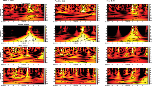
Panels A, B, and C of Figure 1 depict the time-domain evolution of the first- up to the fourth-order moment of the return distributions of equities, gold, and oil, respectively. With respect to the first moment trajectory, we notice that both equity and oil returns exhibit a somewhat similar pattern of consecutive upward and downward trends, with a fairly large amplitude. On the other hand, the amplitude of daily movements in oil returns is utterly high, particularly in the COVID-19 period. In terms of the second moment, oil, equity, and, to a much lesser extent, gold markets appear to suffer from wild price fluctuations under the grip of the pandemic crisis. Such drastic price swings in oil and stock markets are clustered in the stormy period of March-April, which saw oil futures contracts on the NYMEX crashing into negative territory. The skewness plots suggest asymmetry in the return processes, where the magnitude of positive returns looks different from that of negative returns over time, while the kurtosis plots illustrate that the return series are severely leptokurtic, which implies a high likelihood of extreme tail events.

Figure 1. Time evolution of the first four moments of equity, gold, and oil returns.

3.2. Preliminary analysis

At this early stage of analysis, it seems appropriate to shed light on the univariate properties of the moment series. Some descriptive statistics and test results for equity, gold, and oil are shown in Panels A, B, and C, respectively, of Table 1. To gain more insights, we report the statistics for both subsamples. From a row-wise perspective, it is obvious that global gold markets post higher positive average daily returns with lower price volatility than do their stock counterparts, whether prior to or after the outbreak of COVID-19, while oil markets experience negative mean daily returns with huge volatility, especially in the second period. The empirical distributions of equity and oil (gold) returns are skewed to the left (right) with positive excess kurtosis. Paralleling our results, Salisu et al. (2020) find that Brent crude oil returns exhibit negative asymmetry in the pre- and post-COVID-19 announcement periods. Negative skewness coupled with leptokurtosis suggest a higher-than-normal probability of extreme left-tail events (e.g., rare disasters). In terms of the second-order realized moment, $RV$, oil has the largest mean daily realized volatility (i.e., 4.540 and 44.112), as compared to equity and gold over both periods. We also notice that following the advent of the pandemic, realized volatility of oil returns spiked nearly tenfold, which is a glaring manifestation of the recent historic price crash that thrust oil markets into chaos. Likewise, Dutta et al. (2020) and Narayan (2020) find that volatility of oil returns multiplied dramatically during the pandemic crisis. From a column-wise view, all moment series appear to be either positively or negatively skewed and leptokurtic, implying that their underlying distributions are far from being normal. The Jarque-Bera test statistics prove significant at the 0.01 level, providing further evidence against the null hypothesis of normality.

Table 1. Summary statistics and unit root tests

	Mean	Standard deviation	Skewness	Kurtosis	J-B test	Unit root tests
						ADF	KPSS	ZA
Panel A: Equity
RP	0.067	0.760	−0.761	5.029	46.941***	−14.011***	0.031	−10.904*** (21/6/2019)
RC	0.075	1.873	−0.307	5.063	33.408***	−14.153***	0.055	−16.129*** (23/3/2020)
RVP	0.601	0.617	2.412	9.856	512.557***	−3.771**	0.083	−6.763*** (31/7/2019)
RVC	5.287	11.068	3.522	15.802	1.53E+3***	−4.940***	0.085	−5.523** (24/3/2020)
RSKP	−0.073	1.606	0.071	5.683	52.633***	−5.275***	0.047	−13.565*** (12/7/2019)
RSKC	−0.161	1.147	−2.450	18.538	1.91E+3***	−3.904**	0.093	−8.672*** (21/4/2020)
RKUP	12.561	11.661	2.778	11.413	741.294***	−13.016***	0.108	−13.542*** (7/10/2019)
RKUC	8.470	9.265	8.201	88.991	5.52E+4***	−12.281***	0.063	−4.908* (27/7/2020)
Panel B: Gold
RP	0.091	0.729	0.342	5.316	42.520***	−12.579***	0.059	−12.950*** (5/9/2019)
RC	0.167	1.261	0.985	10.182	399.866***	−12.785***	0.044	−7.737*** (30/6/2020)
RVP	0.656	0.569	2.007	7.306	252.697***	−3.874**	0.032	−6.044*** (24/6/2019)
RVC	1.958	2.906	4.104	24.051	3.67E+3***	−5.716***	0.081	−4.133 (8/4/2020)
RSKP	0.017	2.145	0.585	11.641	554.483***	−13.627***	0.047	−14.696*** (11/10/2019)
RSKC	0.029	1.955	−0.093	16.422	1.29E+3***	−14.215***	0.096	−15.333*** (27/7/2020)
RKUP	15.662	21.577	4.254	24.051	3.75E+3***	−4.772***	0.138*	−15.797*** (8/8/2019)
RKUC	13.130	20.969	5.163	32.898	7.21E+3***	−5.754***	0.072	−6.167*** (24/7/2020)
Panel C: Oil
RP	−0.026	1.930	−0.179	5.600	50.236***	−10.681***	0.036	−11.403*** (12/9/2019)
RC	−0.234	6.997	−1.264	14.940	1.07E+3***	−5.209***	0.080	−11.744*** (23/4/2020)
RVP	4.540	12.558	11.959	152.204	1.66E+5***	−4.828***	0.126*	−7.895*** (13/9/2019)
RVC	44.112	132.495	5.867	40.513	1.11E+4***	−5.434***	0.074	−5.311** (26/2/2020)
RSKP	−0.166	2.539	0.907	13.837	880.398***	−11.212***	0.029	−11.344*** (19/8/2019)
RSKC	0.003	3.426	−0.102	14.151	896.678***	−12.252***	0.047	−8.672*** (21/4/2020)
RKUP	17.383	28.405	4.769	30.277	6.08E+3***	−7.812***	0.078	−8.343*** (23/9/2019)
RKUC	21.470	46.141	3.894	17.697	1.99E+3***	−6.232***	0.068	−4.986* (10/4/2020)

Notes: Panels A, B, and C present summary univariate statistics for each of the first four moments of the return distributions of the S&P 500 futures, the COMEX gold futures, and the NYMEX WTI crude oil futures, respectively. The results of normality and unit root tests are also reported in the table. The full sample includes two non-overlapping intervals of equal length, where the first one is labeled as the pre-pandemic period and runs from 28 April 2019 to 30 December 2019, whereas the second one is labeled as the COVID-19 period and extends from 31 December 2019 to 1 September 2020. R, RV, RSK, and RKU denote the ex-post mean, variance, skewness, and kurtosis, respectively. The subscripts P and C refer to the pre-pandemic and COVID-19 periods. J-B denotes the Jarque-Bera test that examines the null hypothesis of normally distributed residuals. ADF is the Augmented Dickey-Fuller test, which examines the null hypothesis of a unit root, whereas KPSS is the Kwiatkowski, Phillips, Schmidt, and Shin test with the null hypothesis of stationarity. For either subsample period, critical values of the ADF (KPSS) test, with both a drift and linear trend, are −4.012, −3.436, and −3.142 (0.216, 0.146, and 0.119) at the 0.01, 0.05, and 0.10 significance levels, respectively. ZA is the Zivot-Andrews structural-break unit-root test, which examines the null hypothesis that a given series is a unit root process against the alternative of a trend-stationary process with a possible structural break in the intercept and the trend (slope) of the series. Break dates are given in parentheses. The appropriate number of lags is identified by the Akaike information criterion (AIC). For either subsample period, critical values for the ZA unit root test with a structural break in both the intercept and trend are −5.570, −5.080, −4.820 at the 0.01, 0.05, and 0.10 significance levels, respectively. ***, ** and * indicate statistical significance at the 0.01, 0.05, and 0.10 levels, respectively.

Standard unit root test statistics are presented in the last three Columns of Table 1. The results of the Augmented Dickey–Fuller (ADF) test (Dickey & Fuller, 1979, 1981) allow us to reject the null hypothesis that a univariate time series possesses a unit root at the 0.05 level or better. When running the KPSS test (Kwiatkowski et al., 1992) as a cross-check, we fail to reject the null hypothesis of stationarity in almost all cases. Overall, these findings confirm that moment series are stationary in their levels. On the other hand, our sample period is fraught with various economic, political, and health shocks, which may give rise to the existence of structural shifts in the individual time series. To account for such a possibility, we perform the Zivot-Andrews (ZA) unit-root test (Zivot & Andrews, 1992), which has the ability of endogenously identifying a single break in the intercept, the slope of the trend function, or both. Once again, the ZA test statistics confirm that the individual moment series are stationary processes at standard significance levels, with a one-time level and trend break. The sole exception is the realized volatility of gold during the pandemic period, which appears to have a unit root. Most break dates are clustered in anxiety-filled months of March, April, and July 2020. The presence of such structural changes justifies our choice of the wavelet analysis, which can adequately be utilized to investigate the time- and frequency-localized information with structural shifts.

We also perform Pearson’s correlation analysis to identify the strength and direction of the associations between the same-order moments of equity, gold, and oil returns. Tables 2 and 3 show the correlation coefficients in the pre-pandemic and COVID-19 periods, respectively. For first period, the first-order moment pair of oil and equity exhibits the largest correlation coefficient of 0.169, which proves positive and statistically significant at the 0.05 level. The remaining pairwise relationships are very small in magnitude and lack statistical significance. For the COVID-19 period, the correlation coefficient of the first-order moment pair of oil and equity becomes stronger, in terms of both magnitude and statistical significance. At the second-order moment level, we find that equity markets are positively correlated with gold and oil counterparts at the 0.01 level, with correlation coefficients of 0.438 and 0.214, respectively, while at the third-moment level, equity and gold are significantly and positively related, with an estimated correlation of 0.172. Across both sample periods, we detect no significant association between gold and oil markets. Besides, the pairwise correlations at the fourth-moment level turn out to be quite low and statistically insignificant. Unlike the classic time-domain correlation analysis, the wavelet coherence technique gives the opportunity to uncover bivariate dynamic interactions, which might be transient in time or could switch directionality across diverse temporal scales.

Table 2. Correlation coefficients during the pre-pandemic period

Panel A: First moments				Panel B: Second moments
	$R_E$	$R_G$	$R_O$		$R{V}_E$	$R{V}_G$	$R{V}_O$
$R_E$	1.000			$R{V}_E$	1.000
$R_G$	0.108 (1.423)	1.000		$R{V}_G$	0.101 (1.337)	1.000
$R_O$	0.169** (2.267)	0.123 (1.632)	1.000	$R{V}_O$	0.021 (0.282)	0.055 (0.723)	1.000
Panel C: Third moments				Panel D: Fourth moments
	$RS{K}_E$	$RS{K}_G$	$RS{K}_O$		$RK{U}_E$	$RK{U}_G$	$RK{U}_O$
$RS{K}_E$	1.000			$RK{U}_E$	1.000
$RS{K}_G$	0.036 (0.477)	1.000		$RK{U}_G$	−0.052 (−0.685)	1.000
$RS{K}_O$	−0.077 (−1.014)	0.049 (0.647)	1.000	$RK{U}_O$	−0.029 (−0.387)	0.025 (0.691)	1.000

Notes: This table provides a snapshot of the pairwise correlation coefficients between the same-order moments of the return distributions of the S&P 500 futures, the COMEX gold futures, and the NYMEX WTI crude oil futures during the pre-pandemic period. R, RV, RSK, and RKU stand for the ex-post mean, variance, skewness, and kurtosis, respectively. The subscripts E, G, and O denote equity, gold, and oil, respectively. The figures given in parentheses are t-statistics. *** indicates statistical significance at the 0.01 level.

Table 3. Correlation coefficients during pandemic period

Panel A: First moments				Panel B: Second moments
	$R_E$	$R_G$	$R_O$		$R{V}_E$	$R{V}_G$	$R{V}_O$
$R_E$	1.000			$R{V}_E$	1.000
$R_G$	−0.123 (−1.625)	1.000		$R{V}_G$	0.438*** (6.377)	1.000
$R_O$	0.349*** (3.370)	−0.090 (−1.183)	1.000	$R{V}_O$	0.214*** (2.865)	0.056 (0.742)	1.000
Panel C: Third moments				Panel D: Fourth moments
	$RS{K}_E$	$RS{K}_G$	$RS{K}_O$		$RK{U}_E$	$RK{U}_G$	$RK{U}_O$
$RS{K}_E$	1.000			$RK{U}_E$	1.000
$RS{K}_G$	0.172** (2.286)	1.000		$RK{U}_G$	0.028 (0.368)	1.000
$RS{K}_O$	−0.016 (−0.212)	−0.107 (−1.419)	1.000	$RK{U}_O$	0.016 (0.215)	0.073 (1.009)	1.000

Notes: This table provides a snapshot of the pairwise correlation coefficients between the same-order moments of the return distributions of the S&P 500 futures, the COMEX gold futures, and the NYMEX WTI crude oil futures during the COVID-19 pandemic. The figures given in parentheses are t-statistics. *** indicates statistical significance at the 0.01 level. For legends, see, Table 2.

4. Methodology

To have a deeper understanding on what the same-order moment interdependence structure between equity, gold, and oil returns looks like under the strain of the global health crisis, we use the wavelet analysis. In contrast to conventional time-series methodologies (i.e., OLS, ARDL, and GARCH models), which are confined to time-domain analysis, and frequency-domain approaches (i.e., Fourier analysis) in which potentially viable information from the time-domain is discarded, the wavelet technique explores concurrently the time-varying and frequency-varying characteristics of the variables under study (Ramsey, 2002). Zapranis and Alexandridis (2008) underscore that a main advantage of this technique is that it can give a proper representation of data with complex structures, without a priori knowledge of the underlying functional form of the data. Moreover, In and Kim (2013) point out that since the vast majority of economic and financial data encompass certain features (e.g., trends, regime shifts, seasonalities, other stochastic processes) belonging to distinct frequency bands, the stringent requirement of stationarity may result in a loss of important information in the data. As a remedy, the wavelet analysis is particularly capable of processing non-stationary signals that tend to display rapid changes. In what follows, we provide a concise account of wavelet coherence and phase-difference techniques.

4.1. Continuous wavelet transform

The continuous wavelet transform (CWT) with the Morlet mother-wavelet function (Morlet et al., 1982) is adopted to address the issues of interest across the time and frequency dimensions. Percival and Walden (2000) and Aguiar-Conraria et al. (2008), among others, indicate that a family of daughter wavelets of some signal evolving in time, x(t), can be generated by dilating and shifting a reference function, $\mathrm{\Psi }$, which is often referred to as the mother wavelet. Mathematically, $\mathrm{\Psi }\left(x\right)$ is expressed as follows:

(9) ${\mathrm{\Psi }}_{u,s}\left(x\right)=\frac{1}{\sqrt{s}}\mathrm{\Psi }\left(\frac{x-u}{s}\right),\phi \left(.\right)\in L^2\left(\mathbb{R}\right),\hspace{0.17em}s\ne 0$(9)

where s and u are the scale (aka dilation) and time (aka translation) parameters, respectively,$L^2\left(\mathbb{R}\right)$ denotes the Hilbert space of square-integrable one-dimensional functions, and $1/\sqrt{s}$ is a factor normalizing the wavelets to guarantee that they have unit variance (i.e.,${{\mathrm{\Psi }}_{u,s}}^2=1$). As pointed out by Rua and Nunes (2009), this factor is important to ensure that different wavelet transforms are comparable across s and u. Corresponding to frequency information, the scale parameter controls the width of the wavelet envelope in the time domain, and, as a consequence, we can obtain stretched or compressed versions of $\mathrm{\Psi }\left(x\right)$. Due to the fact that scale and frequency are inversely proportional, large scales (i.e.,$s>1$) detect low-frequency movements and, hence, reveal coarse information on a large segment of the signal, whereas small scales (i.e.,$s<1$) capture high-frequency oscillations and, thus, are able to disclose detailed information on a small segment of the signal. On the other hand, the translation parameter, u, is employed to advance or delay the wavelet position on the time axis. The value of u influences only the wavelet location in time, but not its bandwidth or duration. Accordingly, through changing u and using different s factors, the whole signal is covered in a more intelligent and adaptive manner.

Torrence and Compo (1998) and Percival and Walden (2000) show that, given a signal or time series x(t), its corresponding CWT is defined by the following convolution:

(10) $W_x\left(u,s\right)={\int }_{-\mathrm{\infty }}^{+\mathrm{\infty }}x\left(t\right){\mathrm{\Psi }}_{u,s}^{\ast }\left(t\right)dt=\frac{1}{\sqrt{s}}{\int }_{-\mathrm{\infty }}^{+\mathrm{\infty }}x\left(t\right){\mathrm{\Psi }}^{\ast }\left(\frac{x-u}{s}\right)dt$(10)

where the asterisk denotes the complex conjugation operator of $\mathrm{\Psi }\left(x\right)$, viz. the basis wavelet function. Eq. (10)(10) $W_x\left(u,s\right)={\int }_{-\mathrm{\infty }}^{+\mathrm{\infty }}x\left(t\right){\mathrm{\Psi }}_{u,s}^{\ast }\left(t\right)dt=\frac{1}{\sqrt{s}}{\int }_{-\mathrm{\infty }}^{+\mathrm{\infty }}x\left(t\right){\mathrm{\Psi }}^{\ast }\left(\frac{x-u}{s}\right)dt$(10) illustrates how x(t) is decomposed into an ensemble of orthonormal basis wavelet functions, ${\mathrm{\Psi }}_{u,s}\left(x\right),$ generated by dilations and translations of $\mathrm{\Psi }\left(x\right)$. In wavelet theory, there are many types of mother wavelets (e.g., Haar, Morlet, Daubechies, Biorthogonal, Meyer, Mexican Hat), each having distinct properties, and thus serving specific purposes. Aguiar-Conraria and Soares (2011) maintain that complex-valued analytic wavelet is considered an appropriate choice to investigate correlations and synchronization of different time series, since its transform demonstrates an outstanding ability of delivering information on both local amplitude and instantaneous phase of the signal. For our work, we apply one of the most popular analytic versions, the Morlet wavelet (a modulated Gaussian function), which is written as:

(11) ${\mathrm{\Psi }}_{{\omega }_0}\left(t\right)=\frac{1}{\sqrt[4]{\pi }}{e}^{i{\omega }_{0}t}{e}^{-t^2/2}$(11)

and its corresponding Fourier transform is expressed as

(12) ${\hat{\mathrm{\Psi }}}_{{\omega }_0}\left(\omega \right)=\sqrt[4]{\pi }\sqrt{2}{e}^{-{\left((\omega -{\omega }_0\right)}^2)/2}$(12)

where $t$ is the non-dimensional time, the term $\sqrt[4]{\pi }$ is a normalization constant ensuring that the wavelet has unit energy, the exponential term $e^{i{\omega }_{0}t}$ represents a complex sinusoid (sine wave), the exponential term $e^{-t^2/2}$ denotes a Gaussian envelope that has unit standard deviation, and ${\omega }_0$ is the central angular frequency of the wavelet that identifies the number of oscillations within the wavelet (Goupillaud et al., 1984). As ${\omega }_0$ increases, we obtain better frequency localization but poorer time localization, and vice versa. Following past studies (e.g., Andrieș et al., 2014; Ferrer et al., 2018; Vacha & Barunik, 2012; Yang et al., 2016), we set ${\omega }_0=6$, by which the admissibility condition of the wavelet transform is fulfilled. Aguiar-Conraria and Soares (2011) emphasize that the Morlet wavelet presents the most desirable compromise between frequency and time localization, due to the equality of their respective radii (i.e., ${\sigma }_{t;{\mathrm{\Psi }}_{{\omega }_0}}={\sigma }_{\omega ;{\mathrm{\Psi }}_{{\omega }_0}}=1/\sqrt{2}$). Based on the CWT, the wavelet power spectrum (WPS), which determines the contribution of the local variance of x(t) at a specific frequency range relative to the total variance of a stochastic process (Fan & Gençay, 2010), is given by:

(13) $WP{S}_x\left(u,s\right)={\left|W_x\left(u,s\right)\right|}^2$(13)

4.2. Wavelet coherency

In addition to its various univariate time-series analysis applications, the wavelet technique can be extended to multivariate frameworks, in which such issues as dynamic patterns of correlation and causality between variables are investigated, not only over time but across frequencies as well. To verify whether or not two same-order moments move in sync, the wavelet coherence method is in place. As shown in Hudgins et al. (1993) and Gençay et al. (2002), let $W_x\left(u,s\right)$ and $W_y\left(u,s\right)$ denote the CWT of two moment time series x(t) and y(t), respectively. Then, we can express their cross-wavelet transform (XWT) as:

(14) $W_{xy}\left(u,s\right)=W_x\left(u,s\right)W_y^{\ast }\left(u,s\right)$(14)

where $W_y^{\ast }\left(u,s\right)$ is the complex conjugation with respect to the CWT of y(t). The cross-wavelet power spectrum, which detects regions in the time-frequency sphere where x(t) and y(t) show high levels of common power (correspondence), is the modulus of XWT as follows:

(15) ${\left|W_{xy}\left(u,s\right)\right|}^2={\left|W_x\left(u,s\right)\right|}^2{\left|W_y^{\ast }\left(u,s\right)\right|}^2$(15)

Based on Eq. (13)(13) $WP{S}_x\left(u,s\right)={\left|W_x\left(u,s\right)\right|}^2$(13) and (15(15) ${\left|W_{xy}\left(u,s\right)\right|}^2={\left|W_x\left(u,s\right)\right|}^2{\left|W_y^{\ast }\left(u,s\right)\right|}^2$(15) ), the wavelet squared coherence is defined as the smoothed cross-wavelet power spectrum of x(t) and y(t), normalized by the product of their respective smoothed WPSs, as follows (Torrence & Webster, 1999):

(16) $R_{xy}^2\left(u,s\right)=\frac{{\left|\mathbb{Q}\left(s^{-1}{W}_{xy}\left(u,s\right)\right)\right|}^2}{\mathbb{Q}\left[s^{-1}{\left|W_x\left(u,s\right)\right|}^2\right]\mathbb{Q}\left[s^{-1}{\left|W_y\left(u,s\right)\right|}^2\right]}$(16)

where $\mathbb{Q}$ represents a smoothing parameter in scale and time, without which the estimates of $R_x^2\left(u,s\right)$ would always be unity across all s and u. Bounded between zero and one ($0\le R_{xy}^2\left(u,s\right)\le 1$), $R_{xy}^2\left(u,s\right)$ constitutes a direct measure of the contemporaneous correlations between x(t) and y(t) at each point in time and for each frequency (Rua, 2010). A value of $R_{xy}^2\left(u,s\right)$ approaching zero (one) is interpreted as evidence of weak (strong) linear association within a specific time-frequency window. Therefore, in contrast to conventional time-series econometric approaches, the wavelet coherence presents an efficient mechanism to carry out a three-dimensional analysis, since it considers simultaneously the time and frequency content of the series, while assessing the degree of dependence between them. In our analysis, we provide an in-depth portrayal of the same-order moment association by not only identifying those areas of the time-frequency plane wherein the same-order moments co-vary, but also determining the strength of their covariation.

Since the theoretical distribution for the wavelet coherence is unknown, we follow Torrence and Compo (1998) and examine the statistical significance of $R_{xy}^2\left(u,s\right)$ using Monte Carlo simulation methods. White (black) colors on the wavelet coherence plots demonstrate a very strong (very weak) co-movement, which suggests that $R_{xy}^2\left(u,s\right)\approx 1$ ($R_{xy}^2\left(u,s\right)\approx 0$). Regions of the time-frequency space wherein $R_{xy}^2\left(u,s\right)$ is statistically significant at our chosen significance level, $\alpha =0.05$, are marked by thick black contours. On the other hand, the thin black line represents the so-called cone of influence (COI), a threshold below which regions of the wavelet spectrum are subject to edge effects. Such effects emerge as the CWT of a finite-length sampled data (e.g., x(t) and y(t)) has border distortions at the beginning and end of the power spectrum. Consequently, edge effects are likely to distort the results (Percival & Walden, 2000). It should be noticed that, when interpreting the results, portions of the wavelet spectrum inside the COI are disregarded in our analysis.

4.3. Wavelet phase difference

Due to its quadratic nature, the wavelet coherence tool is capable of neither identifying the direction of association between x(t) and y(t), nor capturing their potential lead-lag relationships at different frequencies. This is where the wavelet phase difference approach comes into play to complement the role of the wavelet coherence. Basically, the Morlet wavelet function is complex, which implies that the CWT of x(t) can be decomposed into a real portion, $\mathrm{\Re }\left\{W_x\right\}$, and an imaginary portion, $\mathrm{\Im }\left\{W_x\right\}$. In the spirit of Torrence and Webster (1999) and Bloomfield (2013), the phase difference depicting the phase relationship between x(t) and y(t) is written as:

(17) ${\varphi }_{xy}\left(u,s\right)=ta{n}^{-1}\left(\frac{\mathrm{\Im }\left[\mathbb{Q}\left(s^{-1}{W}_{xy}\left(u,s\right)\right)\right]}{\mathrm{\Re }\left[\mathbb{Q}\left(s^{-1}{W}_{xy}\left(u,s\right)\right)\right]}\right),{\varphi }_{xy}\in \left(-\pi ,\pi \right)$(17)

where $\mathrm{\Re }$ and $\mathrm{\Im }$ denote the real and imaginary components, respectively, of the smoothed XWT. A zero-degree phase difference demonstrates synchronization of x(t) with y(t) at a particular time-frequency. On the wavelet coherence plots, ${\varphi }_{xy}\left(u,s\right)$ is symbolized as black rightward, leftward, upward, and downward arrow signs within regions of statistical significance. A rightward (leftward) pointing arrow suggests that x(t) and y(t) are in phase (out of phase); that is, they are positively (negatively) associated, with negligible or no time lag. In terms of the driver-response relationships, an upward pointing arrow implies that the first time series leads the second one, whereas a downward pointing arrow indicates that the second series leads the first one. Accordingly, a diagonally right-up (left-down) arrow means that x(t) positively (negatively) leads y(t), while a diagonally right-down (left-up) arrow suggests that y(t) positively (negatively) leads x(t).

5. Empirical evidence

We first investigate local variations of power for each individual moment series via the auto-wavelet power spectrum. Next, we delve deeper into local co-variability of the same-order moment pairs, utilizing the wavelet coherence phase difference. In three-dimensional visualizations, the wavelet analysis output is shown in Figures 2 through 4.

Figure 2. Continuous wavelet power spectra of the moment time series.

Notes: This figure shows the Morlet wavelet power spectra of the individual time series. Vertical and horizontal axes indicate the frequency bands and investigation period in days, respectively.  

5.1. Continuous wavelet transforms

As elaborated above, the WPS delivers a depiction of the local power (variance) evolution of a given signal in the time-frequency plane. For exposition purposes, each WPS plot is illustrated as a function of three key dimensions, namely frequency (ordinate-axis), time (abscissa-axis), and power. The frequency component is expressed in units of time and embraces 5-time scale levels, of which the shortest level (2–4 days) denotes the highest frequency and the longest level (32–64 days) reflects the lowest frequency. Since market agents have heterogeneous investment horizons, our representative scale bands are classified into three distinct timeframes, where the 2-4- and 4-8-day cycles (i.e., time ranges up to approximately one week) make up the short-term horizon, the 8–16- and 16–32-day cycles (i.e., time ranges up to roughly one month) are related to the medium-term horizon, and the 32–64-day band (i.e., longer than one month) corresponds to the long-term horizon. In their analysis, Boubaker and Raza (2017), Huang et al. (2015), and Phillips and Gorse (2018) adopt similar investment timeframes. The energy of a moment series is translated into color codes, such that white (black) regions evince very high (low) power, whereas shades of red, orange, and yellow indicate a middle degree of power. The power spectra of the individual moment series of equity, gold, and oil returns are given in Panels A, B, and C, respectively, of Figure 2.

For the three markets, the WPS plots of the first- and second-order moments seem to have a great deal of resemblance, since they likewise show high-energy contours concentrated in the first half of 2020 and are extended over multiple frequencies. As indicated in the Introduction section, this period is fraught with cataclysmic and uncertainty-generating events that impinge on many aspects of the global economic and financial landscape. Consequently, such a striking degree of similarity among the power spectra of equity, gold, and oil returns stems, most probably, from their common exposure to the same underlying factors (e.g., the pandemic-induced turmoil in the world’s stock and energy markets). At the mean level, the equity market plot in Panel A reveals a couple of statistically significant and large areas confined between February and May; the first one is of intermediate-to-high power and covers the short- and medium-term scales, and the second one exhibits a relatively high power and is in the low frequency band of 32–64 days. These findings are analogous to those of Sharif et al. (2020), who notice that the Dow Jones Industrial Average (DJIA) index and the WTI crude oil display pockets of statistically significant wavelet power at short-time scales in March 2020. There are also some pockets showing somewhat high variations at the 4-8- and 8–16-day scales in the April-July 2020 period. By the same token, gold and oil returns in Panels B and C, respectively, demonstrate strong levels of variance at high and medium frequencies over the COVID-19 months.

For the most part, the auto-wavelet power spectra of the second-order moment series tend to resemble their counterparts of the first-order moment series. With the onset of the health crisis and the resultant worldwide disruption, volatilities of the three markets display regions of substantial energy at various time horizons. The stock market volatility plot shows a single large zone over the whole span of frequencies, where the variation strength ranges from very high at the long-term scale of 32–64 days to upper-intermediate at short- and medium-term scales. The volatility of gold (oil) returns appears to exhibit the highest level of variation within low and high (high) frequency bands. Consistent with our results, Okorie and Lin (2020) document that the COVID-19 pandemic triggered short-lived fractal contagion effects, in terms of both returns and volatility, on the stock markets of the worst virus-hit countries, over the January-March 2020 period.

In terms of the third-order moment, we observe that the skewness series have a good deal of commonality, as they exhibit considerable power at short- and medium-term scales, primarily prior to the COVID-19 outbreak. Neither at low frequencies nor after March 2020 do we detect significant regions. Specifically, the equity market skewness plot reveals some small areas clustered in the period between July 2019 and February 2020, with intermediate-to-high power. Likewise, the gold and oil counterparts point to several islands reflecting a mostly high level of energy from June 2019 to March 2020.

With respect to the fourth-order moment series, it is evident that pockets of significant energy in the equity and gold plots are located at high and medium frequencies and are scattered over July 2019-February 2020. It should be highlighted that the second half of 2019 witnessed episodes of systemic unrest, the most crucial of which are the escalating trade war between the US and China, interest-rate cuts by the US Federal Reserve, and the drone attack on oil production facilities of Saudi Aramco, the world’s largest crude exporter. The kurtosis plot of oil shows four islands, with an upper-intermediate level of power. The first two are within the 2-4- and 4-8-day scales, whereas the third one is at the medium-term scale of 16–32 days, during February and March 2020. The fourth island is at the low frequency of 32–64 days and spans December 2019-May 2020, coincident with the pandemic outbreak and the ensuing oil market crash. Mazur et al. (2021) find that the overwhelming majority of the S&P 1500 stock universe experienced both extreme negative returns and extreme volatility during March 2020.

5.2. Moment linkages of equity and gold markets

As mentioned in Subsection (3.3), the direction of the arrows on the wavelet coherence plots discloses the phase relationship between each moment pair (e.g., $m_{1,t},m_{2,t}$) in the time-frequency domain. A rightward (leftward) pointing arrow suggests that $m_{1,t}$ and $m_{2,t}$ are in phase (out of phase), with trivial or no time lag. An upward pointing arrow implies that $m_{1,t}$ leads $m_{2,t}$, while a downward pointing arrow indicates that $m_{2,t}$ leads $m_{1,t}$. Thus, $m_{1,t}$ positively (negatively) leads $m_{2,t}$ if the arrows have a right-up (left-down) direction, while $m_{2,t}$ positively (negatively) leads $m_{1,t}$ if the arrows take a right-down (left-up) direction. To develop deeper insights into the lead-lag relationships, we show in Figure 3 contour graphs of the wavelet coherence and phase difference for each of the same-order moment pairs of equity and gold returns. By and large, the coherence and phase difference for the four moment orders turn out to be frequency- and time-dependent.

Figure 3. Cross-wavelet coherence of the first four moment pairs of stock and gold returns.

Notes: This figure depicts the wavelet coherence and phase-difference between each of the first four moment pairs of stock and gold returns. Vertical and horizontal axes show the frequency bands and investigation period in days, respectively.  

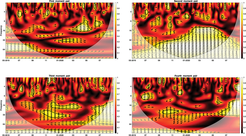
With respect to the cross-mean effects, the predominance of statistically insignificant black- and red-colored areas, especially prior to the pandemic outbreak at medium- and long-term scales, suggests no dependency between stocks and gold. This implies that gold could act as an investment hedge for equities in tranquil times. We notice that, in the high frequency bands of 2–4 and 4–8 days, the nature of the relationship is generally erratic, since arrows inside statistically significant pockets tend to switch directions across the time domain. For instance, arrows point right up in June and November 2019, suggesting that stock returns positively lead gold returns, while they show a right-down direction in February and June 2020, implying that gold returns positively lead stock returns. At the medium-term scale of 8–16 days, we detect two contour regions exhibiting a high degree of cross-wavelet power spectrum during the COVID-19 period. The first one extends over the course of March-May 2020 and its arrows almost point left down, indicating that stock returns negatively lead gold returns. That is, downward trends in equity markets during this unstable period seem to be a precursor of upward trends in the yellow metal counterpart. In fact, the dual exogenous shock of the global health emergency and the later Saudi Arabia-Russia oil price dispute in March-April 2020 sent shudders through stock markets worldwide, prodding investors to shift their capital away from equities to the safe-haven shelter of gold. The second region is in June 2020, with the arrows pointing right down, which means that positive (negative) gold price changes augur well (poorly) for stock markets throughout this month. Likewise, in the medium frequency band of 16–32 days, there is a significant island revealing a relatively high level of coherence in the January-February period. Apparently, contour arrows move again in a right-down direction. On the whole, the positive leading role of gold returns over equities at high and medium frequencies demonstrates that gold may not be a suitable safe-haven asset for equity investors with short- and medium-term horizons, particularly in crisis times. Still, at frequencies greater than a month over the pandemic sample, we observe no significant covariation, which implies that gold could be a weak safe haven for long-term equity investors in periods of global financial turmoil.

In a similar spirit, Bredin et al. (2015) demonstrate the safe-haven (hedge) property of gold during the “Black Monday” crash of 1987 and the global financial crisis of 2008 (non-crisis periods), for horizons up to one year. Employing a DCC-GARCH model, Dutta et al. (2020) document that, amid the oil price crash in April 2020, gold serves as a robust safe-haven investment for global oil markets. Ji et al. (2020) show that gold does not experience fluctuations in the left quantiles of its return distribution during the COVID-19 pandemic, thus validating the safe-haven potential of gold. Baur and McDermott (2016) find that gold demonstrates its safe-haven status following the terrorist attacks in September 2001 and the collapse of Lehman Brothers in September 2008. On the other hand, the results of Cheema et al. (2020) suggest that gold turns out to be an effective safe-haven investment against stock-price declines in the 2007–2009 global financial crisis, but not so in the COVID-19 health crisis. Baur and Trench (2020) establish that corporations in the gold industry (i.e., gold explorers, developers, and miners) are not isolated from the pandemic-triggered stock market crash in March 2020, suggesting that gold equities are not a safe haven.

As far as cross-volatility effects are concerned, there are several small islands over short- and medium-term horizons in the pre-pandemic period. The strength degree of covariation seems to be fairly high in all cases, even though the corresponding arrows show no consistent directional pattern. For example, in June and July 2019, we notice two neighboring regions, wherein the arrows virtually point to the right. This implies that, during this period, equity and gold volatilities move in tandem in the same direction, albeit for only a very short time. In October 2019, the direction of the arrows indicates that the volatility-level pairs are initially out of phase at the shortest time scale of 2–4 days, but become in phase at the subsequent scale of 4–8 days, and then volatility of gold returns positively leads that of stock returns in the medium frequency of 8–16 days. In the pandemic period, there are some tiny islands at high frequency bands, with the arrows taking either a right-up or right-down direction, which is indicative of a positive short-lived lead-lag relationship between the two volatilities. At medium and low frequencies, we observe a huge region overstretched beyond both the time and frequency domains of our analysis. The degree of common power is mostly strong, especially at the long-term scale of 32–64 days. The contour arrows display different paths across scales, which suggest that the cross-volatility effects between stock and gold markets are frequency-dependent. Specifically, in the medium frequency band of 16–32 days, the direction of the phase arrows suggests that volatility of stock returns negatively leads its counterpart of gold returns during the January-June 2020 period, but in the low frequency band of 32–64 days volatility of gold returns positively leads its counterpart of stock returns over the months of October 2019 through June 2020. These findings underscore that price fluctuations in gold markets tend to exert long-run positive effects on stock price volatility, particularly in the aftermath of the pandemic. Accordingly, volatility of gold (stock) returns has a future exacerbating (mitigating) effect on that of equity (gold) returns.

Our cross-volatility results are broadly consistent with those of extant research works. For instance, Balcilar et al. (2021) demonstrate two-way return and volatility transmission effects between the S&P 500 index and gold. Ahmed and Huo (2021) find unilateral shock and volatility spillovers from China’s benchmark stock index, CSI300, to gold futures during July 2012-June 2017. Miyazaki and Hamori (2013) document a unidirectional causality in variance from the S&P 500 index to gold following the onset of the US subprime mortgage crisis in 2007. Based on a battery of stochastic copulas, Boako et al. (2019) find significant price co-jumps between gold and stock markets of Brazil, Russia, Mexico, Indonesia, and Turkey. The results also indicate that the role of gold as a safe-haven asset tends to differ across crisis and non-crisis periods. Utilizing a nonlinear autoregressive distributed lag (NARDL) model, Raza et al. (2016) establish that volatility of gold returns exerts both short- and long-term negative effects on emerging stock markets.

As regards the cross-skewness effects, we can identify several distinct pockets, which feature a relatively strong degree of coherence and are dispersed over the entire sample. As is the case with the cross-volatility effects, the nature of the linkages varies across the time domain at a given scale. For example, in the high frequency band of 4–8 days, the arrows point straight up (down) in June (August) 2019, suggesting that asymmetry risk (e.g., downside risk) of stock (gold) markets leads its counterpart of gold (stock) markets. At the same frequency range, there are two other significant islands. The first one is in March 2020, with its arrows pointing straight left, which implies that asymmetry risks in equity and gold markets move in sync but in opposite trajectories. The second one is in June 2020 and its corresponding arrows exhibit a left-down direction, which indicates that upside and downside crash risks in stock markets negatively lead their respective counterparts of gold markets. As we shift from short- to medium- and long-term scales, we observe that the phase difference becomes more pronounced, since contour regions see an expansion in both time and frequency dimensions. During October 2019-March 2020, the arrows point either straight up or diagonally right up, demonstrating the persistent leading role of asymmetry risks in stock markets over those of gold markets. However, a reversal in the lead-lag relationship in the May-July 2020 period is noted, given the arrowheads mainly point right down. This highlights a clear role reversal between asymmetry risks of stock and gold markets in medium- and low-frequency bands, where the former takes the lead over the latter prior to and in the early months of the COVID-19 outbreak, while the latter leads the former in the subsequent months.

The plot of kurtosis co-movement provides a fairly different picture, since regions delineated by thick contours are scant and sporadic over the time-frequency plane. The coherence strength is predominantly of an upper-intermediate level, and the contour arrows follow heterogeneous paths. Interestingly, the majority of such significant pockets are in the pre-pandemic times. In the period between December 2019 and May 2020, we barely detect areas of common power in all frequencies, a finding implying that the heavy-tail behavior of the distribution of equity returns is uncorrelated with that of gold in this time-frequency space. In June-August 2019 (September-November 2019), fat tail risk (e.g., extreme negative returns) of gold markets seems to negatively (positively) lead its counterpart of equity markets at short- and medium-term scales, because the arrows exhibit almost a left-up (right-down) direction. We note a scale-dependent coherence during the June-July 2020 period, since the kurtosis-level pairs are in phase (out of phase) in the high (medium) frequency band of 4–8 (8–16) days, without significant temporal dependence. Nonetheless, at the subsequent scale (i.e., 16–32 days), arrows show a right-down direction, which corroborates, once again, the leading role of fat tail risk in gold markets over that of stock markets.

In brief, wavelet phase-difference plots of equities and gold provide compelling evidence of cross-market information transmission channeled mainly through the first three moments at medium and low frequencies, particularly in the wake of the global health emergency. By and large, we find that equity (gold) returns and volatility have negative (positive) causal effects on gold (stock) returns and volatility at medium- and long-term scales. Gold may function as a hedge (a weak safe haven) investment for equity investors in tranquil (crisis) times. Asymmetry risk of stock markets positively leads its counterpart of gold markets at medium and low frequencies before and during the initial months of the pandemic, but the relationship becomes reversed in the subsequent sample months.

5.3. Moment linkages of oil and equity markets

In this subsection, we investigate the time-frequency relationship of oil and equity markets. Figure 4 reports the contour graphs of the wavelet coherence and phase difference between the same-order moments of the said markets. A perusal of Figure 4 unveils that cross-mean and cross-volatility dynamics are chiefly characterized by lead-lag relationships, whereas cross-skewness and cross-kurtosis effects are largely characterized by a pattern of zero-degree phase difference.

Figure 4. Cross-wavelet coherence of the first four moment pairs of oil and stock returns.

Notes: This figure depicts the wavelet coherence and phase-difference between each of the first four moment pairs of oil and stock returns. Vertical and horizontal axes show the frequency bands and investigation period in days, respectively.  

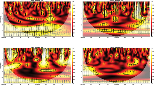
With reference to the first-order moment linkage, the cross-mean effects in the pre-pandemic and pandemic periods resemble each other at short- and medium-term horizons. More specifically, there are several islands dispersed across the full sample period at the short-term scales of 2–4 and 4–8 days, with a comparatively high degree of covariation. The corresponding arrows show either a rightward or leftward direction, suggesting the presence of either a positive or negative contagion effect between oil and stock returns, with minimal or no time lag. Moving from high-frequency to medium-frequency bands, we see some pockets that feature a profound level of coherence and are clustered in June 2019, November 2019, and March–April 2020. The respective arrows seem to point diagonally right up, implying that oil returns positively leads stock returns, for about a two-to-three-week time window. Thus, downward trends in global oil markets could be a harbinger of downward trends in stock markets, and vice versa, over medium-term time cycles. In the low frequency band of 32–64 days, there is a large region mostly reflecting strong coherence and stretching from the start of the sample to June 2020. Once again, positive (negative) oil returns precede positive (negative) stock returns, as the arrows consistently display a right-up direction. Beyond our lowest frequency band of 32–64 days, we observe another significant zone in the period between October 2019 and March 2020. For the most part, the corresponding arrows are north-west facing, which suggests that stock returns negatively lead oil returns. Therefore, it can be inferred that oil returns have a positive leading role over stock returns at medium- and long-term scales, while stock returns have a negative leading role on oil returns for horizons beyond our coarsest time scale in the pandemic period.

Examining the oil-stock nexus under the strain of the COVID-19 outbreak, several studies report results akin to ours. For example, Sharif et al. (2020) provide evidence that the WTI oil prices lead the Dow Jones 30 index at low frequencies. However, Samadi et al. (2021) find a negative co-movement between oil prices and the Tehran Stock Exchange index over short-term horizons. Based on daily data from four major Asian net oil-importing economies (China, India, Japan, and South Korea), Prabheesh et al. (2020) document positive time-varying correlations between oil returns and stock returns, particularly in the early months of the pandemic. Using a panel Vector Autoregressive model, Salisu et al. (2020) demonstrate a bidirectional causality between Brent oil returns and stock returns in the post-COVID-19 announcement period. In the same vein, Wang et al. (2021) propose a dynamic Markov regime switching-copula-extreme value theory (MRS-copula-EVT) model to explore the presence and strength of financial contagion between oil and equities in the US and China. The results confirm the existence of financial contagion between the two markets, with that detected during the COVID-19 crisis being the strongest relative to those found during the 2007–2009 global financial crisis, the 2009–2012 European debt crisis, the 2014 oil crisis, the 2015–2016 China’s stock market crash, and the 2018–2020 Sino-US trade war.

With respect to the second-order moment linkage, we detect several significant pockets that reflect a fairly high level of volatility spillovers and are spread across time and frequency domains. The nature of localized co-movements turns out to be time- and scale-dependent. More explicitly, in July and October 2019 at the short- and medium-term scales of 4–8 and 8–16 days, respectively, volatility of stock returns positively leads volatility of oil returns, since the respective arrows exhibit a mostly right-down direction. Thus, in both months, increases in the stock return volatility precede rises in the oil return volatility for one to three weeks. Nonetheless, in September-November 2019 at the medium-term scale of 16–32 days, the arrowheads become north-west facing, which implies that volatility of stock returns negatively leads that of oil returns. Around December 2019-January 2020, we observe that volatility of stock (oil) returns negatively leads volatility of oil (stock) returns for periods of short-term (medium-term) duration, given the arrows tend to display a left-up (left-down) direction. Over most of the period between February and July 2020, the arrows are north-east facing in nearly all frequency bands, suggesting that the phase-difference relationship is positive and runs from the oil return volatility to the stock return counterpart. In terms of strength, the lead-lag relationship is strong. Moving down to the bottom part of the 32–64-day frequency band, we see a horizontally elongated region spanning September 2019 to April 2020. The direction of the arrows indicates a positive phase-difference relationship, with volatility of stock returns uniformly leading that of oil returns. Hence, we conclude that, during the COVID-19 outbreak, oil price fluctuations maintain a leading role over stock price swings across almost all scales, while the relationship is reversed at very low frequencies.

These results lend support to past research that documents significant volatility transmission between oil and equities in different economies and regions. For example, Bašta and Molnár (2018) demonstrate contemporaneous co-movements (lead-lag relationships) between the implied volatility of the S&P 500 index and its counterpart of oil at high (low) frequencies. X. Liu et al. (2017) establish that mean and volatility spillovers between oil and both of the US and Russian stock markets differ, in terms of direction and strength, across wavelet scales. Ahmed and Huo (2021) report evidence of two-way shock spillovers between the Brent oil and Chinese stock markets, and one-way volatility spillovers from the former to the latter. The results of Yu et al. (2020) show unidirectional volatility spillover effects from the WTI oil price changes to the US DJIA and the Shanghai composite indices, especially in the wake of the global financial crisis. Based on a VAR-GARCH model, Arouri et al. (2012) find that past oil shocks affect volatility of stock prices in six pan-European sector indices. Sarwar et al. (2020) document reciprocal volatility transmission between oil and the Karachi Stock Exchange index, and unidirectional volatility spillovers from oil to the Bombay stock exchange and Shanghai stock exchange indices.

Concerning the third-order moment linkage, it is clear that the vast majority of the significant regions demonstrate a very high degree of strength and are largely localized at short- and medium-term scales across time. For the most part, the corresponding arrows display a rightward or leftward direction, confirming that upside and downside crash risks in oil and stock markets are synchronized and tend to either reinforce or weaken each other across frequencies and time. In more detail, over the June–September 2019 period, the direction of the arrows implies an in-phase coherence at high and medium frequencies. This means that asymmetry risks of both markets move in sync in the same direction, with zero-phase difference, for one to three weeks. Quite similarly, in January–April 2020, we notice a strong positive co-movement stretching over all short- and medium-term scales. There is also a fairly high degree of positive contemporaneous correlation during October 2019–April 2020 at the lowest frequency band and beyond. On the contrary, in December 2019 at short-term horizons and in May–July 2020 at short- and medium-term horizons, asymmetry risks of oil and stock markets move in tandem but in opposite directions since arrows are mostly leftward oriented. Indeed, the prevailing synchronization of asymmetry risks between the two markets at multiple frequencies could potentially arise from their joint exposure to systemic sources of uncertainty (e.g., the record surge in global oil prices due to drone attacks on Saudi refineries in September 2019, the COVID-19 pandemic outbreak, the US stock market crash in March 2020, the Saudi Arabia-Russia oil war and the ensuing sudden price crash in April 2020). As exceptions to the zero-phase difference cases, there appears a couple of significant lead-lag relationships, the first of which is in December 2019 at the short-term scale of 4–8 days, whereas the second one spans February–May 2020 at the medium-term scale of 16–32 days. The former (latter) suggests that the asymmetry risk in stock (oil) markets negatively (positively) leads its counterpart of oil (stock) markets.

In analogy to that of stock and gold markets, the linkage between oil and stock markets via their fourth-order moment appears to be less pronounced, due to the sparse presence of significant contours outside the cone of influence (COI). A careful look at the contour regions reveals that the coherence strength is moderately high, and the arrows are almost north-west, north-east, or south-east oriented. For instance, at high frequencies, fat tail risk of stock markets positively (negatively) leads its counterpart of oil markets in June (August) 2019, since the corresponding arrows show a right-down (left-up) direction. Still, the arrows tend to be north-east facing at medium- and long-term scales (medium-term scales) in June–August 2019 (May–June 2020), suggesting that fat tail risk in oil markets positively leads its counterpart in stock markets. We also notice a positive co-movement during March–April 2020 in the low frequency band of 32–64 days. Finally, barring some tiny islands at short-term scales, fat tail risks of oil and stock returns seem to be independent in the period between September 2019 and end-February 2020 across all frequencies.

In sum, wavelet phase-difference plots indicate the presence of lead-lag correlations between oil and stock markets across time and frequency, predominantly via the first three moments. During the COVID-19 period, oil returns and volatility have substantial causal effects on stock returns and volatility at almost all frequencies, while volatility of stock returns positively leads that of oil returns over longer-term horizons. There is a positive co-movement between asymmetry risks at multiple frequency bands. Heavy tail risks of oil and stock returns are positively related in the stormy period of March–April 2020 at low frequencies.

6. Summary and concluding remarks

With an ever-increasing degree of market connectedness, both regionally and globally, the once-in-a-century COVID-19 pandemic has thrown a pall of gloom and uncertainty on the trajectory of many financial assets. The hefty financial and economic toll, triggered by the global health crisis, has reignited the debate over cross-market linkages and financial contagion, and whether wealth-preserving assets (e.g., gold) can act as a safe haven, even in such times of systemic financial stress. In this study, we run a three-dimensional wavelet analysis to explore the multiscale interdependence structures of the world’s equity, gold, and oil markets under the shadow of the COVID-19 outbreak, with respect to the first four moments of their respective return distributions (i.e., mean, variance, skewness, and kurtosis). More explicitly, we are interested in assessing whether the time-frequency co-movements and lead-lag effects between the same-order moments of the return distributions of equity markets, on the one hand, and both gold and oil markets, on the other, have changed with the spatio-temporal spread of the novel coronavirus. To address these issues, we use 5-minute frequency price data for the S&P 500 futures, the COMEX gold futures, and the NYMEX WTI crude futures. The sample is composed of two non-overlapping intervals of equal length, where the first one runs from 28 April 2019 to 30 December 2019 and is labeled as the pre-pandemic period, whereas the second one is from 31 December 2019 to 1 September 2020 and is regarded as the COVID-19 period. We first apply the wavelet power spectrum to investigate localized variations of power within each individual moment series. Then, both local co-movement and lead-lag relations between the same-order moment of equity-gold and oil-equity pairs are examined via the cross-wavelet coherence and the phase difference, respectively.

Several salient conclusions stand out. First, the coherence and phase difference for each of the same-order moment pairs of equity and gold (oil) returns are frequency- and time-dependent. Second, gold returns have a positive leading role over equity returns at high and medium frequencies during the pandemic period, while, at frequencies greater than one month, there is no significant covariation. This result implies that gold may not be a suitable safe-haven asset for equity investors with short- and medium-term horizons. However, it could be a weak safe haven for long-term equity investors in times of global financial turmoil. Third, price fluctuations in gold (stock) markets exert positive (negative) effects on stock (gold) price fluctuations at low (medium) frequencies, particularly with the onset of the pandemic. Hence, volatility of gold (stock) returns has a future exacerbating (dampening) effect on that of equity (gold) returns. Fourth, there is a role reversal between asymmetry risks of stock and gold markets at medium and low frequency bands, where the former takes the lead over the latter prior to and during the early months of the health crisis, while the latter leads the former in subsequent months. Fifth, the heavy-tail behavior of the distribution of equity returns is uncorrelated with that of gold at almost all scales over most of the sample period. Sixth, oil returns positively lead stock returns at medium- and long-term scales, while stock returns negatively lead oil returns for horizons beyond our coarsest time scale (32–64 days) in the pandemic period. Seventh, volatility of oil prices retains a leading role over stock price swings across most frequencies, but the relationship is reversed at very low frequencies. Eighth, asymmetry risks of oil and stock markets tend to move in sync in the same direction (opposite directions) at short- and medium-term scales in January–April (May–July) 2020. Ninth, the linkage between oil and stock markets via their fourth-order moment appears to be less pronounced.

Our findings offer fresh evidence on the time-frequency moment interdependence between the world’s stock and commodity markets, which bear the economic brunt of the COVID-19 health crisis. Some practical implications can be deduced from the analysis. First, investors should be well cognizant of the mechanisms of information transmission between markets, in terms of higher-order moment risk spillovers. The finding that the stock-gold and oil-stock market pairs are linked not only through mean and volatility, but also through skewness and, sometimes, kurtosis implies that patterns of asymmetry and tail dependence make up a chief concern that should be taken into account when it comes to building cross-asset class portfolios. Moreover, since equities prove sensitive to moment transmission from oil and gold markets, particularly during times of growing uncertainty, investors must pay close attention to price dynamics in these markets, in search of clues about the future course of equity prices.

Second, from a risk management perspective, the results confirm the relevance of the higher-order moments of return distributions as a further potent channel of risk propagation. This suggests that a thorough grasp of the nature and magnitude of market contagion and interdependencies via higher-order moments is essential for developing appropriate hedging strategies. Apparently, the precious yellow metal still stands out as a battle-tested and recession-proof investment alternative. It is also of great importance to explore the time-varying and frequency-varying nature of market interdependencies through moments of their corresponding return distributions, to fulfil the needs of agents with heterogeneous investment time horizons.

Third, the recent oil price tumbles, due to supply glut and COVID-19 outbreak-induced sagging demand, shed doubt on the viability of the black commodity as a safe-haven or a diversifier candidate in the face of equity price swings. Indeed, the coronavirus pandemic and its consequential adverse impacts on oil market dynamics corroborate prior evidence suggesting that the safe-haven characteristic of some investment-asset classes is likely to change over time and, therefore, should be periodically assessed. This sustained assessment is a crucial input for the development of hedging strategies, risk management practices, and optimal portfolios.

Fourth, with the fear of future waves of the pandemic continuing to cast a pall of uncertainty worldwide, policy makers must adopt macroprudential policy toolkits to address the far-reaching socioeconomic repercussions of such a systemic health crisis. In response to lockdowns and disruptions in economic activities, governments and monetary authorities are urged to embark on proper fiscal and monetary stimulus measures, which are thought to be a critical precondition of recovery and growth. Additionally, regulatory bodies should devise innovative strategies intended to maintain capital market resilience and financial stability.

correction

This article has been corrected with minor changes. These changes do not impact the academic content of the article.

Acknowledgment

The authors would like to express their sincere gratitude to the Qatar National Library (QNL) for funding the Open Access of this publication.

Disclosure statement

No potential conflict of interest was reported by the author(s).

Additional information

Funding

The authors received no direct funding for this research.

Notes on contributors

Walid M. A. Ahmed

Walid M. A. Ahmed is an associate professor of Business Administration at the Faculty of Business, Ain Shams University, Cairo, Egypt. Through a channel system between Glasgow Caledonian University, the UK and Ain Shams University, Egypt, he received his Doctorate degree in 2008. His research interests include market volatility dynamics, investor sentiment, and cryptocurrencies. Dr. Walid published many articles in reputed finance and economics journals, such as Applied Financial Economics, Research in International Business and Finance, Resources Policy, The North American Journal of Economics and Finance, Pacific-Basin Finance Journal, and Journal of Economics and Business.

Mohamed A.E. Sleem

Mohamed A.E. Sleem is currently working as a lecturer in finance at school of Management, MSA University, Giza, Egypt. He holds a PhD in Finance from school of management, USM Malaysia, Master of Science degree in EHRM, Sadat Academy, Cairo, Egypt and M.Sc in Information Technology from Nottingham University, UK. He has over 29 years’ experience in teaching finance-related courses at both undergraduate and graduate levels.

Notes

1. Level 1 means that a circuit breaker is triggered to suspend trading for 15 minutes, as the market index drops 7% below its preceding close.

References

- Aguiar-Conraria, L., Azevedo, N., & Soares, M. J. (2008). Using wavelets to decompose the time–frequency effects of monetary policy. Physica A: Statistical Mechanics and Its Applications, 387(12), 2863–30.
- Aguiar-Conraria, L., & Soares, M. J. (2011). Business cycle synchronization and the Euro: A wavelet analysis. Journal of Macroeconomics, 33(3), 477–489.
- Ahmed, A., & Huo, R. (2021). Volatility transmissions across international oil market, commodity futures and stock markets: Empirical evidence from China. Energy Economics, 93, 104741. https://doi.org/10.1016/j.eneco.2020.104741
- Ahmed, W. M. A. (2022). On the higher-order moment interdependence of stock and commodity markets: A wavelet coherence analysis. The Quarterly Review of Economics and Finance, 83, 135–151.
- Albuquerque, R., Koskinen, Y., Yang, S., & Zhang, C. (2020). Resiliency of environmental and social stocks: An analysis of the exogenous COVID-19 market crash. The Review of Corporate Finance Studies, cfaa011, https://doi.org/10.1093/rcfs/cfaa011
- Amaya, D., Christoffersen, P., Jacobs, K., & Vasquez, A. (2015). Does realized skewness predict the cross-section of equity returns? Journal of Financial Economics, 118(1), 135–167.
- Ambros, M., Frenkel, M., Huynh, T. L. D., & Kilinc, M. (2021). COVID-19 pandemic news and stock market reaction during the onset of the crisis: Evidence from high-frequency data. Applied Economics Letters, 28(19), 1686–1689.
- Andersen, T. G., & Bollerslev, T. (1998). Answering the skeptics: Yes, standard volatility models do provide accurate forecasts. International Economic Review, 39(4), 885–905. https://www.jstor.org/stable/2527343
- Andersen, T. G., Bollerslev, T., Diebold, F. X., & Labys, P. (2001). The distribution of realized exchange rate volatility. Journal of the American Statistical Association, 96(453), 42–55.
- Andersen, T. G., Bollerslev, T., Diebold, F. X., & Labys, P. (2003). Modeling and forecasting realized volatility. Econometrica, 71(2), 579–626.
- Andersen, T. G., Bollerslev, T., & Huang, X. (2011). A reduced form framework for modeling volatility of speculative prices based on realized variation measures. Journal of Econometrics, 160(1), 176–189.
- Andrieș, A. M., Ihnatov, I., & Tiwari, A. K. (2014). Analyzing time–frequency relationship between interest rate, stock price and exchange rate through continuous wavelet. Economic Modelling, 41(August), 227–238.
- Andrikopoulos, A., Samitas, A., & Kougepsakis, K. (2014). Volatility transmission across currencies and stock markets: GIIPS in crisis. Applied Financial Economics, 24(19), 1261–1283.
- Arditti, F. D. (1967). Risk and the required return on equity. The Journal of Finance, 22(1), 19–36. https://www.jstor.org/stable/2977297
- Arditti, F. D., & Levy, H. (1975). Portfolio efficiency analysis in three moments multiperiod case. The Journal of Finance, 30(3), 797–809. https://www.jstor.org/stable/2326859
- Arouri, M. H., Jouini, J., & Nguyen, D. K. (2012). On the impacts of oil price fluctuations on European equity markets: Volatility spillover and hedging effectiveness. Energy Economics, 34(2), 611–617. https://doi.org/10.1016/j.eneco.2011.08.009
- Atif, M., Rabbani, M. R., Bawazir, H., Hawaldar, I. T., Chebab, D., Karim, S., & AlAbbas, A. (2022). Oil price changes and stock returns: Fresh evidence from oil exporting and oil importing countries. Cogent Economics & Finance, 10(1). https://doi.org/10.1080/23322039.2021.2018163
- Baker, S. R., Bloom, N., Davis, S. J., & Terry, S. J. (2020). COVID-induced economic uncertainty. NBER Working Paper No. 26983. https://www.nber.org/papers/w26983
- Balcilar, M., Ozdemir, Z. A., & Ozdemir, H. (2021). Dynamic return and volatility spillovers among S&P 500, crude oil, and gold. International Journal of Finance and Economics, 26(1), 153–170. https://doi.org/10.1002/ijfe.1782
- Barndorff-Nielsen, O. E., & Shephard, N. (2002). Econometric analysis of realized volatility and its use in estimating stochastic volatility models. Journal of the Royal Statistical Society: Series B, 64(2), 253–280. https://www.jstor.org/stable/3088799
- Bašta, M., & Molnár, P. (2018). Oil market volatility and stock market volatility. Finance Research Letters, 26, 204–214.
- Baur, D. G., & McDermott, T. K. J. (2016). Why is gold a safe haven? Journal of Behavioral and Experimental Finance, 10, 63–71.
- Baur, D. G., & Trench, A. (2020). Not all gold shines in crisis times- COVID-19 evidence. http://dx.doi.org/10.2139/ssrn.3677925
- Beckmann, J., Berger, T., & Czudaj, R. (2015). Does gold act as a hedge or a safe haven for stocks? A smooth transition approach. Economic Modelling, 48, 16–24.
- Bekiros, S., Nguyen, D. K., Uddin, G. S., & Sjö, B. (2016). On the time scale behavior of equity-commodity links: Implications for portfolio management. Journal of International Financial Markets Institutions and Money, 41, 30–46.
- Bloomfield, P. (2013). Fourier Analysis of Time Series: An Introduction (2nd ed.). John Wiley and Sons.
- Boako, G., Tiwari, A. K., Ibrahim, M., & Ji, Q. (2019). Analysing dynamic dependence between gold and stock returns: Evidence using stochastic and full-range tail dependence copula models. Finance Research Letters, 31.
- Bollerslev, T., Sizova, N., & Tauchen, G. (2012). Volatility in equilibrium: Asymmetries and dynamic dependencies. Review of Finance, 16(1), 31–80.
- Bollerslev, T., Todorov, V., & Xu, L. (2015). Tail risk premia and return predictability. Journal of Financial Economics, 118(1), 113–134.
- Bonato, M., Gupta, R., Lau, C. K. M., & Wang, S. (2020). Moments-based spillovers across gold and oil markets. Energy Economics, 89, 104799.
- Bordalo, P., Gennaioli, N., & Shleifer, A. (2012). Salience theory of choice under risk. Quarterly Journal of Economics, 127(3), 1243–1285.
- Boubaker, H., & Raza, S. A. (2017). A wavelet analysis of mean and volatility spillovers between oil and BRICS stock markets. Energy Economics, 64, 105–117.
- Bredin, D., Conlon, T., & Potì, V. (2015). Does gold glitter in the long-run? Gold as a hedge and safe haven across time and investment horizon. International Review of Financial Analysis, 41, 320–328.
- Chan, K. F., Gray, P., & Campen, B. (2008). A new approach to characterizing and forecasting electricity price volatility. International Journal of Forecasting, 24(4), 728–743.
- Charlot, P., & Marimoutou, V. (2014). On the relationship between the prices of oil and the precious metals: Revisiting with a multivariate regime-switching decision tree. Energy Economics, 44, 456–467.
- Cheema, M. A., Faff, R. W., & Szulczuk, K. (2020). The 2008 global financial crisis and COVID-19 pandemic: How safe are the safe haven assets? Covid Economics, Vetted and Real-Time Papers, 34, 88–115. http://dx.doi.org/10.2139/ssrn.3642945
- Clements, A. E., & Todorova, N. (2016). Information flow, trading activity and commodity futures volatility. Journal of Futures Markets, 36(1), 88–104.
- Cont, R. (2001). Empirical properties of asset returns: Stylized facts and statistical issues. Quantitative Finance, 1(2), 223–236.
- Corbet, S., Hou, G., Hu, Y., Oxley, L., & Xu, D. (2021). Pandemic-related financial market volatility spillovers: Evidence from the Chinese COVID-19 epicentre. International Review of Economics and Finance, 71, 55–81.
- Cui, J., Maghyereh, A., Goh, M., & Zou, H. (2022). Risk spillovers and time-varying links between international oil and China’s commodity futures markets: Fresh evidence from the higher-order moments. Energy, 238(Part B), 121751.
- Dai, P. F., Xiong, X., Liu, Z., Huynh, T. L. D., & Sun, J. (2021). Preventing crash in stock market: The role of economic policy uncertainty during COVID-19. Financial Innovation, 7(1), 1–15.
- Das, D., Kumar, S. B., Tiwari, A. K., Shahbaz, M., & Hasim, H. M. (2018). On the relationship of gold, crude oil, stocks with financial stress: A causality-in-quantiles approach. Finance Research Letters, 27, 169–174.
- Del Brio, E. B., Mora-Valencia, A., & Perote, J. (2017). The kidnapping of Europe: High-order moments’ transmission between developed and emerging markets. Emerging Markets Review, 31, 96–115.
- Dickey, D. A., & Fuller, W. A. (1979). Distribution of the estimators for autoregressive time-series with a unit roots. Journal of the American Statistical Association, 74, 427–431. https://www.jstor.org/stable/2286348
- Dickey, D. A., & Fuller, W. A. (1981). Likelihood ratio statistics for autoregressive time series with a unit root. Econometrica, 49(4), 1057–1072. https://www.jstor.org/stable/1912517
- Diebold, F. X., & Yilmaz, K. (2012). Better to give than to receive: Predictive directional measurement of volatility spillovers. International Journal of Forecasting, 28(1), 57–66.
- Dittmar, R. F. (2002). Nonlinear pricing kernels, kurtosis preference, and evidence from the cross-section of equity returns. The Journal of Finance, 57(1), 369–403.
- Do, H. X., Brooks, R., & Treepongkaruna, S. (2015). Realized spill-over effects between stock and foreign exchange market: Evidence from regional analysis. Global Finance Journal, 28, 24–37.
- Do, H. X., Brooks, R., Treepongkaruna, S., & Wu, E. (2016). Stock and currency market linkages: New evidence from realized spillovers in higher moments. International Review of Economics and Finance, 42, 167–185.
- Dutta, A., Das, D., Jana, R. K., & Vo, X. V. (2020). COVID-19 and oil market crash: Revisiting the safe haven property of gold and Bitcoin. Resources Policy, 69, 101816.
- Ederington, L. H. (1979). The hedging performance of the new futures markets. The Journal of Finance, 34(1), 157–170.
- Elgammal, M. M., Ahmed, W. M. A., & Alshami, A. (2021). Price and volatility spillovers between global equity, gold, and energy markets prior to and during the COVID-19 pandemic. Resources Policy, 74, 102334.
- Fan, Y., & Gençay, R. (2010). Unit root tests with wavelets. Econometric Theory, 26(5), 1305–1331. https://www.jstor.org/stable/40800884
- Ferrer, R., Jammazi, R., Bolós, V. J., & Benítez, R. (2018). Interactions between financial stress and economic activity for the U.S.: A time- and frequency-varying analysis using wavelets. Physica A: Statistical Mechanics and Its Applications, 492, 446–462.
- Finta, M. A., & Aboura, S. (2020). Risk premium spillovers among stock markets: Evidence from higher-order moments. Journal of Financial Markets, 49, 100533.
- Gençay, R., Selçuk, F., & Whitcher, B. (2002). An introduction to wavelets and other filtering methods in finance and economics. Academic Press.
- Goupillaud, P., Grossmann, A., & Morlet, J. (1984). Cycle-octave and related transforms in seismic signal analysis. Geoexploration, 25(1), 85–102.
- Greenwood-Nimmo, M., Nguyen, V. H., & Rafferty, B. (2016). Risk and return spillovers among the G10 currencies. Journal of Financial Markets, 31, 43–62.
- Härdle, W. K., Wang, W., & Yu, L. (2016). TENET: Tail-Event driven NETwork risk. Journal of Econometrics, 192(2), 499–513.
- Hashmi, A. R., & Tay, A. S. (2007). Global regional sources of risk in equity markets: Evidence from factor models with time-varying conditional skewness. Journal of International Money and Finance, 26(3), 430–453.
- He, X., Takiguchi, T., Nakajima, T., & Hamori, S. (2020). Spillover effects between energies, gold, and stock: The United States versus China. Energy & Environment, 31(8), 1416–1447.
- Hou, Y., & Li, S. (2020). Volatility and skewness spillover between stock index and stock index futures markets during a crash period: New evidence from China. International Review of Economics and Finance, 66, 166–188.
- Huang, S., An, H., Gao, X., & Huang, X. (2015). Identifying the multiscale impacts of crude oil price shocks on the stock market in China at the sector level. Physica A: Statistical Mechanics and Its Applications, 434, 13–24.
- Hudgins, L., Friehe, C., & Mayer, M. (1993). Wavelet transforms and atmospheric turbulence. Physics Review Letters, 71(20), 3279–3282.
- Hung, N. T., & Vo, X. V. (2021). Directional spillover effects and time-frequency nexus between oil, gold and stock markets: Evidence from pre and during COVID-19 outbreak. International Review of Financial Analysis, 76, 101730.
- Huynh, T. L. D., Foglia, M., Nasir, M. A., & Angelini, E. (2021). Feverish sentiment and global equity markets during the COVID-19 pandemic. Journal of Economic Behavior & Organization, 188, 1088–1108.
- Huynh, T. L. D., Foglia, M., & Doukas, J. A. (2022). COVID-19 and tail-event driven network risk in the eurozone. Finance Research Letters, 44, 102070.
- In, F., & Kim, S. (2013). An introduction to wavelet theory in finance: A wavelet multiscale approach. World Scientific Publishing Co. Pte. Ltd.
- International Energy Agency. (2020). Oil Market Report - July 2020. https://www.iea.org/reports/oil-market-report-july-2020
- Ji, Q., Zhang, D., & Zhao, Y. (2020). Searching for safe-haven assets during the COVID-19 pandemic. International Review of Financial Analysis, 71, 101526.
- Jiang, S., Li, Y., Lu, Q., Wang, S., & Wei, Y. (2022). Volatility communicator or receiver? Investigating volatility spillover mechanisms among Bitcoin and other financial markets. Research in International Business and Finance, 59, 101543.
- Khalifa, A. A. A., Hammoudeh, S., & Otranto, E. (2014). Patterns of volatility transmissions within regime switching across GCC and global markets. International Review of Economics and Finance, 29, 512–524.
- Kim, S., & Kim, C. S. (2010). Do S&P 500 and KOSPI move together?: A functional regression approach. Korean Economic Review, 26(2), 401–430.
- Kinateder, H., Campbell, R., & Choudhury, T. (2021). Safe haven in GFC versus COVID-19: 100 turbulent days in the financial markets. Finance Research Letters, 43, 101951.
- Kliber, A., & Łęt, B. (2022). Degree of connectedness and the transfer of news across the oil market and the European stocks. Energy, 239, 122171.
- Kozhan, R., Anthony, N., & Schneider, P. (2012). The skew risk premium in the equity index market. Review of Financial Studies, 26(9), 2174–2203.
- Kraus, A., & Litzenberger, R. (1976). Skewness preference and the valuation of risk assets. The Journal of Finance, 31(4), 1085–1100. https://www.jstor.org/stable/2326275
- Kwiatkowski, D., Phillips, P. C. B., Schmidt, P., & Shin, Y. (1992). Testing the null hypothesis of stationarity against the alternative of a unit root: How sure are we that economic time series have a unit root? Journal of Econometrics, 54(1–3), 159–178. https://doi.org/10.1016/0304-4076(92)90104-Y
- Lee, S. S., & Hannig, J. (2010). Detecting jumps from Lévy jump diffusion processes. Journal of Financial Economics, 96(2), 271–290.
- Liu, L., Patton, A. J., & Sheppard, K. (2015). Does anything beat 5‐minute RV? A comparison of realized measures across multiple asset classes. Journal of Econometrics, 187(1), 293–311.
- Liu, X., An, H., Huang, S., & Wen, S. (2017). The evolution of spillover effects between oil and stock markets across multi-scales using a wavelet-based GARCH–BEKK model. Physica A: Statistical Mechanics and Its Applications, 465, 374–383.
- Lucas, A., & Klaassen, P. (1998). Extreme returns, downside risk, and optimal asset allocation. The Journal of Portfolio Management, 25(1), 71–79.
- Mazur, M., Dang, M., & Vega, M. (2021). COVID-19 and the March 2020 stock market crash. Evidence from S&P1500. Finance Research Letters, 38, 101690. https://doi.org/10.1016/j.frl.2020.101690
- Mensi, W., Yousaf, I., Vo, X. V., & Kang, S. H. (2022). Asymmetric spillover and network connectedness between gold, BRENT oil and EU subsector markets. Journal of International Financial Markets, Institutions and Money, 76, 101487.
- Ming, L., Shen, Y., Yang, S., Zhu, S., & Zhu, H. (2019). Does gold serve as a hedge for the stock market in China? Evidence from a time-frequency analysis. Emerging Markets Finance and Trade, 56(3), 659–672.
- Miyazaki, T., & Hamori, S. (2013). Testing for causality between the gold return and stock market performance: Evidence for ‘gold investment in case of emergency’. Applied Financial Economics, 23(1), 27–40.
- Morlet, J., Arehs, G., Fourgeau, I., & Giard, D. (1982). Wave propagation and sampling theory—Part I: Complex signal and scattering in multilayered media. Geophysics, 47(2), 203–221.
- Narayan, P. K. (2020). Oil price news and COVID-19—Is there any connection? Energy Research Letters, 1(1), 1–5.
- Okorie, D. I., & Lin, B. (2020). Stock markets and the COVID-19 fractal contagion effects. Finance Research Letters, 38, 101640.
- Özdemir, O. (2022). Cue the volatility spillover in the cryptocurrency markets during the COVID-19 pandemic: Evidence from DCC-GARCH and wavelet analysis. Financial Innovation, 8(1), 12.
- Palandri, A. (2015). Do negative and positive equity returns share the same volatility dynamics? Journal of Banking and Finance, 58, 486–505.
- Peiró, A. (1999). Skewness in financial returns. Journal of Banking and Finance, 23(6), 847–862.
- Percival, D. B., & Walden, A. T. (2000). Wavelet methods for time series analysis. Cambridge University Press.
- Phillips, R. C., & Gorse, D. (2018). Cryptocurrency price drivers: Wavelet coherence analysis revisited. PLoS ONE, 13(4), e0195200.
- Prabheesh, K. P., Padhan, R., & Garg, B. (2020). COVID-19 and the oil price-stock market nexus: Evidence from net oil-importing countries. Energy RESEARCH LETTERS, 1(2), 1–6.
- Press, S. J. (1967). A compound events model for security prices. The Journal of Business, 40(3), 317–335. https://www.jstor.org/stable/2351754
- Ramsey, J. B. (2002). Wavelets in economics and finance: Past and future. Studies in Nonlinear Dynamics and Econometrics, 6(3), 1–29. https://doi.org/10.2202/1558-3708.1090
- Raza, N., Shahzad, S. J. H., Tiwari, A. K., & Shahbaz, M. (2016). Asymmetric impact of gold, oil prices and their volatilities on stock prices of emerging markets. Resources Policy, 49, 290–301.
- Reboredo, J. C., Rivera-Castro, M. A., & Ugolini, A. (2016). Downside and upside risk spillovers between exchange rates and stock prices. Journal of Banking and Finance, 62, 76–96.
- Rossi, E., & de Magistris, P. S. (2013). Long memory and tail dependence in trading volume and volatility. Journal of Empirical Finance, 22, 94–112.
- Rua, A., & Nunes, L. C. (2009). International comovement of stock market returns: A wavelet analysis. Journal of Empirical Finance, 16(4), 632–639.
- Rua, A. (2010). Measuring comovement in the time–frequency space. Journal of Macroeconomics, 32(2), 685–691.
- Rubinstein, M. E. (1973). The fundamental theorem of parameter-preference security valuation. The Journal of Financial and Quantitative Analysis, 8(1), 61–69. https://www.jstor.org/stable/2329748
- Sahabuddin, M., Hassan, M. F., Tabash, M. I., Al-Omari, M. A., Alam, M. K., & Islam, F. T. (2022). Co-movement and causality dynamics linkages between conventional and Islamic stock indexes in Bangladesh: A wavelet analysis. Cogent Business and Management, 9(1), 2034233.
- Saiti, B., Bacha, O. I., & Masih, M. (2016). Testing the conventional and Islamic financial market contagion: Evidence from wavelet analysis. Emerging Markets Finance and Trade, 52(8), 1832–1849.
- Salisu, A. A., Ebuh, G. U., & Usman, N. (2020). Revisiting oil-stock nexus during COVID-19 pandemic: Some preliminary results. International Review of Economics and Finance, 69, 280–294.
- Samadi, A. H., Owjimehr, S., & Halafi, Z. N. (2021). The cross-impact between financial markets, Covid-19 pandemic, and economic sanctions: The case of Iran. Journal of Policy Modeling, 431, 34–55. https://doi.org/10.1016/j.jpolmod.2020.08.001
- Sarwar, S., Tiwari, A. K., & Tingqiu, C. (2020). Analyzing volatility spillovers between oil market and Asian stock markets. Resources Policy, 66, 101608.
- Scott, R., & Horvath, P. (1980). On the direction of preference for moments of higher order than the variance. The Journal of Finance, 35(4), 915–919. https://www.jstor.org/stable/2327209
- Shaikh, I., & Huynh, T. L. D. (2022). Does disease outbreak news impact equity, commodity, and foreign exchange market? Investors’ fear of the pandemic COVID-19. Journal of Economic Studies, 49(4), 647–664. https://doi.org/10.1108/JES-10-2020-0503
- Sharif, A., Aloui, C., & Yarovaya, L. (2020). COVID-19 pandemic, oil prices, stock market, geopolitical risk and policy uncertainty nexus in the US economy: Fresh evidence from the wavelet-based approach. International Review of Financial Analysis, 70, 101496.
- Sharma, G. D., Sarker, T., Rao, A., Talan, G., & Jain, M. (2022). Revisiting conventional and green finance spillover in post-COVID world: Evidence from robust econometric models. Global Finance Journal, 51, 100691.
- Simkowitz, M. A., & Beedles, W. L. (1978). Diversification in a three-moment world. Journal of Financial and Quantitative Analysis, 13(5), 927–941. https://www.jstor.org/stable/2330635
- Sortino, F., & van der Meer, R. (1991). Downside risk. The Journal of Portfolio Management, 17(4), 27–31.
- Torrence, C., & Compo, G. (1998). A practical guide to wavelet analysis. Bulletin of the American Meteorological Society, 79(1), 61–78.
- Torrence, C., & Webster, P. J. (1999). Interdecadal Changes in the ENSO–Monsoon System. Journal of Climate, 12(8), 2679–2690.
- Uddin, G. S., Hernandez, J. A., Shahzad, S. J. H., & Kang, S. H. (2020). Characteristics of spillovers between the US stock market and precious metals and oil. Resources Policy, 66, 101601.
- Umar, Z., Yousaf, I., & Aharon, D. Y. (2021). The relationship between yield curve components and equity sectorial indices: Evidence from China. Pacific-Basin Finance Journal, 68, 101591.
- Vacha, L., & Barunik, J. (2012). Co-movement of energy commodities revisited: Evidence from wavelet coherence analysis. Energy Economics, 34(1), 241–247.
- Wang, H., Yuan, Y., & Wang, T. (2021). The dynamics of cross-boundary fire—Financial contagion between the oil and stock markets. Journal of Futures Markets, 41(10), 1655–1673.
- World Economic Forum. (2020). Mad March: How the stock market is being hit by COVID-19. https://www.weforum.org/agenda/2020/03/stock-market-volatility-coronavirus/
- Yang, L., Cai, X. J., Zhang, H., & Hamori, S. (2016). Interdependence of foreign exchange markets: A wavelet coherence analysis. Economic Modelling, 55, 6–14.
- Yarovaya, L., Matkovskyy, R., & Jalan, A. (2022). The COVID-19 black swan crisis: Reaction and recovery of various financial markets. Research in International Business and Finance, 59, 101521.
- Yoon, S.-M., Al Mamun, M., Uddin, G. S., & Kang, S. H. (2019). Network connectedness and net spillover between financial and commodity markets. The North American Journal of Economics and Finance, 48, 801–818.
- Yousaf, I. (2021). Risk transmission from the COVID-19 to metals and energy markets. Resources Policy, 73, 102156.
- Yu, L., Zha, R., Stafylas, D., He, K., & Liu, J. (2020). Dependences and volatility spillovers between the oil and stock markets: New evidence from the copula and VAR-BEKK-GARCH models. International Review of Financial Analysis, 68, 101280.
- Zapranis, A., & Alexandridis, A. (2008). Modeling the temperature time‐dependent speed of mean reversion in the context of weather derivatives pricing. Applied Mathematical Finance, 15(4), 355–386.
- Zhu, P., Tang, Y., Wei, Y., & Lu, T. (2021). Multidimensional risk spillovers among crude oil, the US and Chinese stock markets: Evidence during the COVID-19 epidemic. Energy, 231, 120949.
- Zivot, E., & Andrews, D. W. K. (1992). Further evidence on the great crash, the oil price shock and the unit root hypothesis. Journal of Business and Economic Statistics, 10, 251–270. https://doi.org/10.2307/1391541