A Bitcoin price prediction model assuming oscillatory growth and lengthening cycles

Abstract

This article’s motivation is to understand the volatile Bitcoin price increase. The objective is to develop price estimation methods. The methodology is to present five differential equation models estimated against the 23 July 2010–21 June 2021 Bitcoin data. The findings are that Gompertz growth fits the damped oscillations and lengthening cycles well, and tracks the early data better with the weighted least squares method. Gompertz growth combined with charged capacitor growth tracks the early data even better. Logistic growth is too slow to track the early data. Logistic growth combined with charged capacitor growth to some extent tracks the early data. Pure charged capacitor growth is unrealistic. The dates for the future bull market maxima depend to a low degree on the growth model carrying capacity approached asymptotically, assumed to match gold at $10 trillion, and to be 50 times higher. The implications for traders are to focus on the large standard deviations. Investors should understand the growth potential compared with other asset classes. Regulators should ensure financial stability by focusing on the fluctuations. Central banks should adjust the money supply while acknowledging. Bitcoin competition. Collective units should understand Bitcoin growth models to determine whether to accept Bitcoin transactions.

Keywords:

• Bitcoin
• logistic growth
• oscillation
• lengthening cycles
• price prediction
• differential equations
• least squares method

JEL Classification:

• Numbers: C5
• E3

1. Introduction

1.1. Background

Since the genesis block was mined on 3 January 2009 at 18:15:05 UTC, the Bitcoin price has increased above 100% per year subject to fluctuations. Understanding the nature of the growth and fluctuations is of paramount importance. A variety of opinions emerge on how the Bitcoin price evolves into the future. Skeptics believe the Bitcoin price is in a bubble and will collapse. Others see Bitcoin, accompanied with layer 2 solutions for scaling (e.g., the Lightning Network) and layer 3 solutions for interoperability, as the future dominant means of payment, measure of value, medium of exchange, basis of credit, standard of postponed payment, store of value, and possibly unit of account. Other cryptocurrencies may contribute. The decentralized nature of Bitcoin, where anyone can run a node which stores the entire blockchain, emerges as a competitor to traditional media of exchange and stores of value which require an intermediary. Thus for example El Salvador on 7 September 2021 and the Central African Republic on 27 April 2022 accepted Bitcoin as legal tender. Cryptocurrencies and their underlying ledger technologies currently impact how most central banks develop digital currencies. These developments can be expected to reshape the financial system.

1.2. Contribution

This article’s motivation, objectives, research hypotheses, and research questions are as follows. First, the Bitcoin price has increased apparently unpredictably since 3 January 2009, which suggests a need both to understand the evolution so far and to predict the future evolution. Second, applying Bitcoin’s price data since 23 July 2010, methods are developed to estimate and understand this price evolution as accurately as possible. The Bitcoin empirics are such that the methods involve growth models, while accounting for oscillations and lengthening cycles. Third, two different Bitcoin carrying capacities are considered, assumed to express reasonable outer limits for what can be expected over the next decades. Fourth, five differential equation models are compared against each other to determine which is best, applying the least squares method and the weighted least squares method. Fifth, the methods are used to predict the future Bitcoin price and future bull marked maxima.

More specifically, first, a generalized logistic growth model is presented, which depicts the Bitcoin price’s growth with four characteristics: logistic growth, damped oscillation, retracement in bear markets, and lengthening cycles. Second, a generalized charged capacitor growth is introduced with damped oscillation, retracement in bear markets, and lengthening cycles. Third, the article introduces what the authors believe are two hitherto unknown theoretical combinations of growth models, i.e., logistic growth combined with charged capacitor growth, and Gompertz growth combined with charged capacitor growth. This gives five models which are solved analytically and analyzed numerically.

The least squares method is applied to estimate the models’ parameters. Supplementation is made with the weighted least squares method since the Bitcoin price variance increases over time, exhibiting heteroscedasticity. Based on the three bull market local maxima and three bear market local minima during the period 23 July 2010–21 June 2021, the scaling of the inverse of the cycle length of the sine oscillations, and the scaling of the inverse of the degree of lengthening of each subsequent cycle, are estimated. The amplitude of the oscillations, and the start time adjustment parameter for the sine oscillations, are estimated to predict the future bull market local maxima and bear market local minima.

The article outperforms other alternative approaches and adds to our knowledge in various ways. First, the dynamic nature of the Bitcoin price is such that differential time equations are especially well suited. Such differential equations do exist in the literature, but are perhaps in the minority. Second, the Bitcoin price is not only characterized by dynamics, but by dynamic growth. Hence this article focuses explicitly on growth models. Third, the Bitcoin price is characterized by dynamic oscillatory growth with lengthening cycles, which is explicitly incorporated into the analysis.

1.3. Literature

The existing literature predicts the Bitcoin price applying various methods, occasionally using differential equations, and more generally accounting for statistics, econometrics, machine learning, neural network, deep learning, etc. The literature is divided into five groups, i.e., 1. Differential equations, 2. Bitcoin price dynamics, 3. Gompertz growth and Metcalfe’s Law, 4. Machine learning, and 5. Neural network, deep learning and memory models. This article correlates most with the first two groups, while introducing growth with damped oscillatory and lengthening cycles. The last three groups are included for broader positioning.

1.3.1. Differential equations

Relatively few studies apply differential equations to predict the Bitcoin price. K. S. Chen and Huang (2020) adopt a stochastic differential equation to capture the evolution of the Bitcoin price 2015–2018. Their differential equation considers the instantaneous expected return, the instantaneous volatility, and jumps focusing explicitly on the crash after the 17 December 2017 and Brownian motion. They focus on the jump risk distribution of the Bitcoin price and Bitcoin options pricing and hedging. Such a focus on jumps is implicitly present in the current article which determines moves back and forth between bull market maxima and bear market minima. Jalali and Heidari (2020) adopt grey system theory and propose a first order differential equation to predict the Bitcoin price. The approach requires an appropriate time frame. They focus explicitly on five-day predictions. That differs from the current article which predicts over any future time horizon. Wang and Wang (2020) introduce a partial differential equation model to predict the Bitcoin price January 1–31 December 2017. They incorporate the daily Bitcoin transaction volumes and google trends index, and the spatial heterogeneity of chainlet clusters, which proceeds beyond this article’s focus. This article differs from these other articles applying differential equations by focusing explicitly on the Bitcoin price growth patterns. That is, the differential equations consider the Bitcoin price, two different Bitcoin carrying capacities, damped oscillations, lengthening cycles, and bull market maxima and bear market minima for five different growth models.

1.3.2. Bitcoin price dynamics

The following articles pertain to Bitcoin price dynamics, but with a different focus and applying other models than in the current article, thus implicitly illustrating a gap in the literature. Statistics and econometrics are widely used methods to forecast the Bitcoin price. Begusic et al. (2018) demonstrate slowly decaying tails in the distributions of Bitcoin returns, and a power law with 2 < α < 2.5, which means heavier tails than for stocks with alpha around 3. Such slowly decaying tails seem consistent with damped oscillations, and heavy tails seem consistent with the substantial fluctuations between maxima and minima, found in the current article.

Caporale et al. (2019) apply statistical methods for 2013–2018. They find that the frequency of price overreactions is informative about Bitcoin price movements and the Bitcoin price exhibits no seasonality. Their approach constitutes an alternative way of assessing the drive towards bull market maxima and bear market minima.

Roy et al. (2018) apply 2013–2017 data and present an autoregressive integrated moving average model which predicts the Bitcoin price volatility with 90% accuracy, thus also capturing fluctuations between maxima and minima.

Indera et al. (2017) apply 2012–2017 data and develop a multi-layer perceptron-based non-linear autoregressive model to predict the Bitcoin price with good accuracy. They generate moving averages, account for input and output lags, and apply regression analysis, validation and fitting tests. They focus less on the timing and magnitudes of the maxima and minima than the current article.

Cretarola and Figa-Talamanca (2021) apply a continuous time stochastic model to determine how bubbles in the Bitcoin price in 2012–2013 and in 2017 are linked to the correlation between the market attention to Bitcoin and the Bitcoin return being above a threshold, known as market exuberance. Such bubbles are yet another way of assessing bull market maxima. Jana et al. (2021) apply 2013–2019 data to forecast the Bitcoin price through a differential evolution-based regression framework, shown to be superior to six advanced predictive modeling algorithms. Instead of differential equations, they apply polynomial regression on time series.

Further studies consider market attention, market sentiment, active addresses, etc. for Bitcoin price prediction, which is a broader focus than in the current article. Sabalionis et al. (2021) found that the amount of active addresses impacts the Bitcoin and Ethereum prices more than other factors such as google search interest and number of tweets. Haffar and Le Fur (2021) applied a structural vector error correction model to determine that the Bitcoin price in the short run is influenced positively by Asian emerging countries and negatively by North America. In the long run, the influence is negative from all countries in Asia and the Pacific, and positive from Europe. This article adopts a wider range of Bitcoin price data than the above articles, applying growth models to explain and predict the Bitcoin price.

1.3.3. Gompertz growth and Metcalfe’s Law

The quick initial increase in Gompertz growth (commonly used for e.g. tumor growth; see Yorke et al. (1993)) is found to be descriptive in the current article. Two other articles have also identified Gompertz growth as descriptive. Peterson (2018) applies the Gompertz curve to capture the inflationary impacts of the creation of new Bitcoin, shown to follow Metcalfe’s Law. Patel et al. (2020) found that the price of cryptocurrencies follows a Gompertz growth function, which links the traditional time-value-of-money concepts to Metcalfe’s law, and that the growth rate of users impacts the Bitcoin price. This article extends this focus to other growth models, i.e., logistic growth, charged capacitor growth, and combinations of growth models, accounting for damped oscillation and lengthening cycles.

1.3.4. Machine learning

Several studies apply machine learning methods to explain and predict the Bitcoin price. Chevallier et al. (2021) applied six machine learning algorithms to parameterize and disentangle the non-stationary behavior of the Bitcoin price data, as an alternative to classical parameter models. They suggest that machine learning does not teach how to trade due to the substantial Bitcoin price variability, and that long term holding may be preferable. Such a suggestion seems compatible with the current article which determines overall 2010–2021 growth, interrupted by substantial downturns towards bear market minima. Dutta et al. (2020) present a framework of machine learning forecasting methods to predict the Bitcoin’s price. They compare various approaches, arguing that the gated recurring unit model with a recurrent dropout performs best. Z. Chen et al. (2020) predict the Bitcoin price with various frequencies data via machine learning techniques. They also incorporate high-dimension features like property and network, trading and market, attention, etc. They show that statistical methods perform better than machine learning algorithms, reaching accuracy of 66% and 65.3%, respectively.

Some articles combine machine learning and econometrics. Mudassir et al. (2020) developed high-performance machine learning-based classification and regression models to predict the Bitcoin price. The models have accuracy of 65% and 64% for next-day forecast and seventh–ninetieth-day forecast, respectively. Gupta and Nain (2021) use time series involving moving averages, autoregressive integrated moving averages, and multiple machine learning approaches including Support Vector Machine, Long Short Term Memory and Gated Recurrent Unit. They compare these models to determine their accuracy. The machine learning approach is challenging since it requires appropriate data input. Long term forecasting is challenging. Instead of machine learning, this article applies differential equations and least squares methods which more directly cause price explanation and prediction.

1.3.5. Neural network, deep learning and memory models

Recent articles adopt neural networks and deep learning to predict the Bitcoin price, which enables the analysis of instructed data including documents, images, and texts. Ji et al. (2019) explored the performance of a deep neural network model, a Long Short-Term Memory model, and a Convolutional Neural Network model, to predict the Bitcoin price. They show that the deep neural network model predicts price increases and decreases nicely, and that classification models are more effective than regression models. Patel et al. (2020) present a Long Short Term Memory and Gated Recurrent Unit based hybrid cryptocurrency prediction model to predict the price of Litecoin and Monero. They found that the model accurately predicts the prices.

Hua (2020) compares the accuracy of predicting the Bitcoin price via Long Short Term Memory model and an Autoregressive Integrated Moving Average model. He finds that the former performs better, but requires more time to train the neural network. Cocco et al. (2021) compared several approaches to predict the Bitcoin price. They show that two-stage frameworks usually outperform one-stage frameworks, except for one-stage Bayesian Neural Network. Jaquart et al. (2021) proposed a stochastic neural network model based on random walk to predict the price of cryptocurrencies. The approach induces a layer-wise randomness into the neural networks to capture market volatility. Using multi-layer perceptron and Long Short Term memory models, they found that the proposed models perform well compared with deterministic models.

Chkili (2021) applies a long memory model and a Markov switching model to determine the Bitcoin price volatility, which relates to the focus in the current article of assessing fluctuations between maxima and minima. A common challenge faced by the deep learning approach is finding the optimal network hyperparameters. That contrasts with the current article which applies least squares methods to estimate the parameters.

1.4 Article organization

Section 2 presents the materials and methods. Section 3 analyzes the model and presents the results. Section 4 discusses the results. Section 5 concludes.

2. Materials and methods

This section identifies and develops the differential equations believed to capture the Bitcoin price evolution most accurately.

2.1. Nomenclature

Parameters

$k$Growth rate, $k\in \mathbb{R}$

$K$Carrying capacity, $K\ge 0$

$\nu$Parameter for generalized logistic growth impacting near which asymptote maximum growth occurs, $\nu \ge 0$

$\lambda$Adjustment parameter for combined generalized logistic and charged capacitor growth, $\lambda \in \mathbb{R}$

$\alpha$Oscillation amplitude, expressing strength of bull and bear markets, $\alpha \in \mathbb{R}$

$\omega$Scaling of the inverse of the cycle length of the sine oscillations, $\omega \in \mathbb{R}$

$\gamma$Scaling of the inverse of the degree of lengthening of each subsequent cycle, $\gamma \in \mathbb{R}$

$\delta$Start time adjustment parameter relative to time $t=t_0$ for the oscillation of the Sin function, $\gamma \in \mathbb{R}$

$t_0$Initial time $t$

$T$Final time $t$

$p_0$Initial price $p$ at time $t=t_0$

Independent variable

$t$Time

Dependent variable

$p$Price

2.2. Generalized logistic growth

This section generalizes Richards’ (1959) model for growth modeling to

(1) $\begin{array}{cc}\hspace{0.17em}& \frac{\mathrm{\partial }p}{\mathrm{\partial }t}=\left(k+\alpha Sin\left(\omega {\left(t-t_0\right)}^{\gamma }+\delta \right)\right)p\left(1-{\left(\frac{p}{K}\right)}^v\right)\\ \hspace{0.17em}& \Rightarrow p=\frac{K}{{\left(1+{\left(\frac{K}{p_0}-1\right)}^{\nu }{e}^{-\left(k+Q\right)\nu \left(t-t_0\right)}\right)}^{1/\nu }},\underset{t\to \mathrm{\infty }}{lim}p=K,\\ \hspace{0.17em}& Q\equiv \frac{i\alpha }{2\gamma }\left(e^{i\delta }\underset{1}{\overset{\mathrm{\infty }}{\int }}\frac{e^{i\omega {\left(t-t_0\right)}^{\gamma }q}}{q^{\frac{\gamma -1}{\gamma }}}dq-e^{-i\delta }\underset{1}{\overset{\mathrm{\infty }}{\int }}\frac{e^{-i\omega {\left(t-t_0\right)}^{\gamma }q}}{q^{\frac{\gamma -1}{\gamma }}}dq\right),i\equiv \sqrt{-1}\end{array}$(1)

where $\mathrm{\partial }$ means partial differentiation, $t$ means time, $t_0$ is the start time, $k\in \mathbb{R}$ is the growth rate which expresses how quickly the price $p$ changes, and $K\ge 0$ is the carrying capacity, defined as the maximum sustainable price $p$. Equation (1)(1) $\begin{array}{cc}\hspace{0.17em}& \frac{\mathrm{\partial }p}{\mathrm{\partial }t}=\left(k+\alpha Sin\left(\omega {\left(t-t_0\right)}^{\gamma }+\delta \right)\right)p\left(1-{\left(\frac{p}{K}\right)}^v\right)\\ \hspace{0.17em}& \Rightarrow p=\frac{K}{{\left(1+{\left(\frac{K}{p_0}-1\right)}^{\nu }{e}^{-\left(k+Q\right)\nu \left(t-t_0\right)}\right)}^{1/\nu }},\underset{t\to \mathrm{\infty }}{lim}p=K,\\ \hspace{0.17em}& Q\equiv \frac{i\alpha }{2\gamma }\left(e^{i\delta }\underset{1}{\overset{\mathrm{\infty }}{\int }}\frac{e^{i\omega {\left(t-t_0\right)}^{\gamma }q}}{q^{\frac{\gamma -1}{\gamma }}}dq-e^{-i\delta }\underset{1}{\overset{\mathrm{\infty }}{\int }}\frac{e^{-i\omega {\left(t-t_0\right)}^{\gamma }q}}{q^{\frac{\gamma -1}{\gamma }}}dq\right),i\equiv \sqrt{-1}\end{array}$(1) expresses that the price $p$ changes logistically from $p_0$, $p_0\ge 0$, at the initial time $t=t_0$ towards $p=K$ as time $t$ approaches infinity. The parameter $\nu$, $\nu \ge 0$, impacts near which asymptote maximum growth occurs.

Whereas Richards (1959) assumes a constant growth rate, (1) supplements the growth rate $k$ with a Sin function and four additional parameters. The Sin function oscillates between +1 and −1 to reflect bull markets with increased growth rate when the Sin function is positive, and bear markets with decreased growth rate when the Sin function is negative.

The parameter $\alpha \in \mathbb{R}$ expresses the strength of the bull and bear markets, and thus the size of the positive and negative amplitudes in the oscillations. Equation (1)(1) $\begin{array}{cc}\hspace{0.17em}& \frac{\mathrm{\partial }p}{\mathrm{\partial }t}=\left(k+\alpha Sin\left(\omega {\left(t-t_0\right)}^{\gamma }+\delta \right)\right)p\left(1-{\left(\frac{p}{K}\right)}^v\right)\\ \hspace{0.17em}& \Rightarrow p=\frac{K}{{\left(1+{\left(\frac{K}{p_0}-1\right)}^{\nu }{e}^{-\left(k+Q\right)\nu \left(t-t_0\right)}\right)}^{1/\nu }},\underset{t\to \mathrm{\infty }}{lim}p=K,\\ \hspace{0.17em}& Q\equiv \frac{i\alpha }{2\gamma }\left(e^{i\delta }\underset{1}{\overset{\mathrm{\infty }}{\int }}\frac{e^{i\omega {\left(t-t_0\right)}^{\gamma }q}}{q^{\frac{\gamma -1}{\gamma }}}dq-e^{-i\delta }\underset{1}{\overset{\mathrm{\infty }}{\int }}\frac{e^{-i\omega {\left(t-t_0\right)}^{\gamma }q}}{q^{\frac{\gamma -1}{\gamma }}}dq\right),i\equiv \sqrt{-1}\end{array}$(1) simplifies to Richards' (1959) model when $\alpha =0$ which eliminates the sine oscillations causing $Q=0$.

The parameter $\omega \in \mathbb{R}$ scales the inverse of the cycle length of the sine oscillations. Higher $\omega$ gives shorter cycle length, since $\omega$ is multiplied with time $t$, and higher $\omega$ means that each cycle with length $2\pi$ gets completed more quickly.

The parameter $\gamma \in \mathbb{R}$ scales the inverse of the degree of lengthening of each subsequent cycle as time $t$ progresses. Lower $\gamma$ gives more lengthening of each subsequent cycle as time $t$ progresses. Mathematically, if we consider $\gamma =1$ as a common benchmark giving linear oscillatory progression through time $t$, decreasing gamma below 1 causes $\omega {\left(t-t_0\right)}^{\gamma }<\omega \left(t-t_0\right)$, and hence more time $t$ is needed for each subsequent cycle with length $2\pi$ to be completed. In contrast, increasing gamma above 1 causes $\omega {\left(t-t_0\right)}^{\gamma }>\omega \left(t-t_0\right)$, and hence less time $t$ is needed for each subsequent cycle with length $2\pi$ to be completed. Equation (1)(1) $\begin{array}{cc}\hspace{0.17em}& \frac{\mathrm{\partial }p}{\mathrm{\partial }t}=\left(k+\alpha Sin\left(\omega {\left(t-t_0\right)}^{\gamma }+\delta \right)\right)p\left(1-{\left(\frac{p}{K}\right)}^v\right)\\ \hspace{0.17em}& \Rightarrow p=\frac{K}{{\left(1+{\left(\frac{K}{p_0}-1\right)}^{\nu }{e}^{-\left(k+Q\right)\nu \left(t-t_0\right)}\right)}^{1/\nu }},\underset{t\to \mathrm{\infty }}{lim}p=K,\\ \hspace{0.17em}& Q\equiv \frac{i\alpha }{2\gamma }\left(e^{i\delta }\underset{1}{\overset{\mathrm{\infty }}{\int }}\frac{e^{i\omega {\left(t-t_0\right)}^{\gamma }q}}{q^{\frac{\gamma -1}{\gamma }}}dq-e^{-i\delta }\underset{1}{\overset{\mathrm{\infty }}{\int }}\frac{e^{-i\omega {\left(t-t_0\right)}^{\gamma }q}}{q^{\frac{\gamma -1}{\gamma }}}dq\right),i\equiv \sqrt{-1}\end{array}$(1) also simplifies to Richards’ (1959) model at the limit when $\underset{\gamma \mathrm{\infty }}{lim}Q=0$, since each subsequent cycle gets completed immediately and thus the sine oscillations have no impact.

The parameter $\delta \in \mathbb{R}$ adjusts the start time at time $t=0$ for the oscillation of the Sin function. For example, if $\delta =0$, $Sin\left(\omega t^{\gamma }+\delta \right)=0$ when $t=0$, which gives zero amplitude and thus no impact of the Sin function at time $t=0$.

2.2.1. Conventional logistic growth

Inserting $\nu =1$ into (1) gives conventional logistic growth (Lotka, 1924; Verhulst, 1845) with oscillation, retracement in bear markets, and lengthening cycles, where both the initial value asymptote $t=t_0$ and the future value asymptote $t\to \mathrm{\infty }$ are approached symmetrically.

2.2.2 Gompertz growth

Inserting the limit $\nu ->0^{+}$ into (1) gives conventional Gompertz (1825, p. 518) logistic growth with oscillation, retracement in bear markets, and lengthening cycles, i.e.,

(2) $\begin{array}{cc}\hspace{0.17em}& \frac{\mathrm{\partial }p}{\mathrm{\partial }t}=\left(k+\alpha Sin\left(\omega {\left(t-t_0\right)}^{\gamma }+\delta \right)\right)pLn\left(\frac{K}{p}\right)\Rightarrow p=K{\left(\frac{p_0}{K}\right)}^{{\mathrm{e}}^{-\left(k+R\right)\left(t-t_0\right)}},\\ & \\ & R\equiv \frac{\mathrm{i}\alpha }{2\gamma \left(t-t_0\right){\omega }^{\frac{1}{\gamma }}}\left(\begin{array}{c}{\mathrm{e}}^{\frac{\mathrm{i}\left(\pi +2\gamma \delta \right)}{2\gamma }}\left(\underset{-\mathrm{i}{\left(t-t_0\right)}^{\gamma }\omega }{\overset{\mathrm{\infty }}{\int }}{q}^{\frac{1}{\gamma }-1}{e}^{-q}dq-1\right)\\ -{\mathrm{e}}^{-\frac{\mathrm{i}\left(\pi +2\gamma \delta \right)}{2\gamma }}\left(\underset{\mathrm{i}{\left(t-t_0\right)}^{\gamma }\omega }{\overset{\mathrm{\infty }}{\int }}{q}^{\frac{1}{\gamma }-1}{e}^{-q}dq-1\right)\end{array}\right)\end{array}$(2)

where $Ln$ is the natural logarithm, and the initial value asymptote $t=t_0$ is approached more quickly than the future value asymptote $t\to \mathrm{\infty }$. Equation (2)(2) $\begin{array}{cc}\hspace{0.17em}& \frac{\mathrm{\partial }p}{\mathrm{\partial }t}=\left(k+\alpha Sin\left(\omega {\left(t-t_0\right)}^{\gamma }+\delta \right)\right)pLn\left(\frac{K}{p}\right)\Rightarrow p=K{\left(\frac{p_0}{K}\right)}^{{\mathrm{e}}^{-\left(k+R\right)\left(t-t_0\right)}},\\ & \\ & R\equiv \frac{\mathrm{i}\alpha }{2\gamma \left(t-t_0\right){\omega }^{\frac{1}{\gamma }}}\left(\begin{array}{c}{\mathrm{e}}^{\frac{\mathrm{i}\left(\pi +2\gamma \delta \right)}{2\gamma }}\left(\underset{-\mathrm{i}{\left(t-t_0\right)}^{\gamma }\omega }{\overset{\mathrm{\infty }}{\int }}{q}^{\frac{1}{\gamma }-1}{e}^{-q}dq-1\right)\\ -{\mathrm{e}}^{-\frac{\mathrm{i}\left(\pi +2\gamma \delta \right)}{2\gamma }}\left(\underset{\mathrm{i}{\left(t-t_0\right)}^{\gamma }\omega }{\overset{\mathrm{\infty }}{\int }}{q}^{\frac{1}{\gamma }-1}{e}^{-q}dq-1\right)\end{array}\right)\end{array}$(2) simplifies to Richards’ (1959) model when $R=0$.

2.3. Generalized charged capacitor growth

This section assumes generalized charged capacitor growth with damped oscillation, retracement in bear markets, and lengthening cycles, with growth rate $\left(k+\alpha Sin\left(\omega {\left(t-t_0\right)}^{\gamma }+\delta \right)\right)$, i.e.,

(3) $\begin{array}{cc}\hspace{0.17em}& \frac{\mathrm{\partial }p}{\mathrm{\partial }t}=\left(k+\alpha Sin\left(\omega {\left(t-t_0\right)}^{\gamma }+\delta \right)\right)\left(1-{\left(\frac{p}{K}\right)}^{\nu }\right)\\ \hspace{0.17em}& \Rightarrow p=InverseFunction\left[{-}_2^{\hspace{0.17em}}{F}_1\left(1,\frac{1}{v},1+\frac{1}{v},{\left(\frac{\mathrm{\#}}{K}\right)}^{\nu }\right)\mathrm{\#}\mathrm{\&}\right]\\ \hspace{0.17em}& \left[-\left(k+Q\right)\left(t-t_0\right)-{p_0}_2^{\hspace{0.17em}}{F}_1\left(1,\frac{1}{v},1+\frac{1}{v},{\left(\frac{p_0}{K}\right)}^{\nu }\right)\right],\underset{t\to \mathrm{\infty }}{lim}p=K\end{array}$(3)

where $Q$ is defined in (1), which simplifies to

(4) $\begin{array}{cc}\hspace{0.17em}& \frac{\mathrm{\partial }p}{\mathrm{\partial }t}=\left(k+\alpha Sin\left(\omega {\left(t-t_0\right)}^{\gamma }+\delta \right)\right)\left(1-\frac{p}{K}\right)\\ \hspace{0.17em}& \Rightarrow p=K-\left(K-p_0\right)e^{-\left(k+Q\right)\left(t-t_0\right)/K},\underset{t\to \mathrm{\infty }}{lim}p=K\end{array}$(4)

when $\nu =1$, and simplifies to $\frac{\mathrm{\partial }p}{\mathrm{\partial }t}=0\Rightarrow p=p_0$, i.e., no growth, when $\nu =0$. The function ${\hspace{0.17em}}_2^{\hspace{0.17em}}{F}_1\left(a,b,c,z\right)$ is hypergeometric with power series assuming $\left|z\right|<1$. The Mathematica (www.wolfram.com) notation in (3) is as follows: $InverseFunction\left[f\right]$ is the inverse of the function $f$, defined so that $InverseFunction\left[f\right]\left[y\right]$ gives the value of $x$ for which $f\left[x\right]=y$. The symbol $\mathrm{\#}$ is the first argument supplied to a pure function, so that $f\left[\mathrm{\#}\right]\mathrm{\&}\left[x\right]$ evaluates to $f\left[x\right]$. The symbol & expresses the end of the argument. Charged capacitor growth expresses a quick initial price increase, due to the high value of the right-hand side of the differential Equation (3)(3) $\begin{array}{cc}\hspace{0.17em}& \frac{\mathrm{\partial }p}{\mathrm{\partial }t}=\left(k+\alpha Sin\left(\omega {\left(t-t_0\right)}^{\gamma }+\delta \right)\right)\left(1-{\left(\frac{p}{K}\right)}^{\nu }\right)\\ \hspace{0.17em}& \Rightarrow p=InverseFunction\left[{-}_2^{\hspace{0.17em}}{F}_1\left(1,\frac{1}{v},1+\frac{1}{v},{\left(\frac{\mathrm{\#}}{K}\right)}^{\nu }\right)\mathrm{\#}\mathrm{\&}\right]\\ \hspace{0.17em}& \left[-\left(k+Q\right)\left(t-t_0\right)-{p_0}_2^{\hspace{0.17em}}{F}_1\left(1,\frac{1}{v},1+\frac{1}{v},{\left(\frac{p_0}{K}\right)}^{\nu }\right)\right],\underset{t\to \mathrm{\infty }}{lim}p=K\end{array}$(3) when $p_0$ is low.

2.4. Combined generalized logistic and charged capacitor growth

Combining (3) and (1) gives

(5) $\begin{array}{cc}\hspace{0.17em}& \frac{\mathrm{\partial }p}{\mathrm{\partial }t}=\left(k+\alpha Sin\left(\omega {\left(t-t_0\right)}^{\gamma }+\delta \right)\right)p^{\lambda }\left(1-{\left(\frac{p}{K}\right)}^{\nu }\right)\\ \hspace{0.17em}& \Rightarrow p=InverseFunction\left[{\frac{-{\mathrm{\#}}^{1-\lambda }}{1-\lambda }}_2^{\hspace{0.17em}}{F}_1\left(1,\frac{1-\lambda }{v},1+\frac{1-\lambda }{v},{\left(\frac{\mathrm{\#}}{K}\right)}^{\nu }\right)\mathrm{\&}\right]\\ \hspace{0.17em}& \left[-\left(k+Q\right)\left(t-t_0\right)-{\frac{p_0^{1-\lambda }}{1-\lambda }}_2^{\hspace{0.17em}}{F}_1\left(1,\frac{1-\lambda }{v},1+\frac{1-\lambda }{v},{\left(\frac{p_0}{K}\right)}^{\nu }\right)\right],\underset{t\to \mathrm{\infty }}{lim}p=K\end{array}$(5)

where the price $p$ is raised to an exponent $\lambda$, $\lambda \in \mathbb{R}$, and ${\hspace{0.17em}}_2^{\hspace{0.17em}}{F}_1\left(a,b,c,z\right)$ is defined in (3). The adjustment parameter $\lambda$ can be thought of as weighing generalized logistic growth (conventional logistic growth and Gompertz growth) and charged capacitor growth against each other. Equation (5)(5) $\begin{array}{cc}\hspace{0.17em}& \frac{\mathrm{\partial }p}{\mathrm{\partial }t}=\left(k+\alpha Sin\left(\omega {\left(t-t_0\right)}^{\gamma }+\delta \right)\right)p^{\lambda }\left(1-{\left(\frac{p}{K}\right)}^{\nu }\right)\\ \hspace{0.17em}& \Rightarrow p=InverseFunction\left[{\frac{-{\mathrm{\#}}^{1-\lambda }}{1-\lambda }}_2^{\hspace{0.17em}}{F}_1\left(1,\frac{1-\lambda }{v},1+\frac{1-\lambda }{v},{\left(\frac{\mathrm{\#}}{K}\right)}^{\nu }\right)\mathrm{\&}\right]\\ \hspace{0.17em}& \left[-\left(k+Q\right)\left(t-t_0\right)-{\frac{p_0^{1-\lambda }}{1-\lambda }}_2^{\hspace{0.17em}}{F}_1\left(1,\frac{1-\lambda }{v},1+\frac{1-\lambda }{v},{\left(\frac{p_0}{K}\right)}^{\nu }\right)\right],\underset{t\to \mathrm{\infty }}{lim}p=K\end{array}$(5) simplifies to generalized logistic growth in (1) when $\lambda =1$, simplifies to Gompertz growth in (2) when $\lambda =1$ at the limit $v\to 0^{+}$, and simplifies to generalized charged capacitor growth in (3) when $\lambda =0$. Hence $0<\lambda <1$ enables growth intermediate between quick generalized charged capacitor growth when $\lambda =0$, and slower generalized logistic growth when $\lambda =1$. Compared with generalized logistic growth in (4) when $\lambda >1$, initial growth when the price $p$ is low is damped since $p^{\lambda }$ in (5) is comparatively low, and eventual growth is amplified more when the price $p$ is high since $p^{\lambda }$ in (5) is comparatively high.

2.4.1 Combined logistic and charged capacitor growth

Inserting $\nu =1$ into (5) gives combined conventional logistic growth and generalized charged capacitor growth expressed as

(6) $\begin{array}{cc}\hspace{0.17em}& \frac{\mathrm{\partial }p}{\mathrm{\partial }t}=\left(k+\alpha Sin\left(\omega {\left(t-t_0\right)}^{\gamma }+\delta \right)\right)p^{\lambda }\left(1-\frac{p}{K}\right)\\ \hspace{0.17em}& \Rightarrow p=InverseFunction\left[{\frac{{\mathrm{\#}}^{1-\lambda }}{K\left(1-\lambda \right)}}_2^{\hspace{0.17em}}{F}_1\left(1,1-\lambda ,2-\lambda ,\frac{\mathrm{\#}}{K}\right)\mathrm{\&}\right]\\ \hspace{0.17em}& \left[\frac{\left(k+Q\right)\left(t-t_0\right)}{K}+K^{-\lambda }\underset{0}{\overset{p_0/K}{\int }}\frac{q^{-\lambda }}{1-q}dq\right],\underset{t\to \mathrm{\infty }}{lim}p=K\end{array}$(6)

2.4.2 Combined Gompertz and charged capacitor growth

Inserting the limit $v\to 0^{+}$ into (5) gives combined Gompertz growth and generalized charged capacitor growth expressed as

(7) $\begin{array}{cc}\hspace{0.17em}& \frac{\mathrm{\partial }p}{\mathrm{\partial }t}=\left(k+\alpha Sin\left(\omega {\left(t-t_0\right)}^{\gamma }+\delta \right)\right)p^{\lambda }Ln\left(\frac{K}{p}\right)\\ \hspace{0.17em}& \Rightarrow p=InverseFunction\left[e^{\left(1-\lambda \right)Ln\left(K\right)}\underset{\left(1-\lambda \right)Ln\left(\frac{K}{\mathrm{\#}}\right)}{\overset{\mathrm{\infty }}{\int }}\frac{e^{-q}}{q}dq\mathrm{\&}\right]\\ \hspace{0.17em}& \left[\left(k+Q\right)\left(t-t_0\right)+K^{1-\lambda }\underset{\left(1-\lambda \right)Ln\left(\frac{K}{p_0}\right)}{\overset{\mathrm{\infty }}{\int }}\frac{e^{-q}}{q}dq\right],\underset{t\to \mathrm{\infty }}{lim}p=K\end{array}$(7)

3. Results

The results are presented over seven subsections. Sections 3.1 and 3.2 assume no oscillation and estimate and predict the Bitcoin price with the various methods developed in the previous section. Sections 3.3 and 3.4 generate results needed to account for oscillation. These results pertain to Bitcoin price maxima and minima, cycle length and cycle lengthening. Sections 3.5 and 3.6 allow for oscillation and predict the Bitcoin price with the various methods. Section 3.7 estimates future bull market maxima.

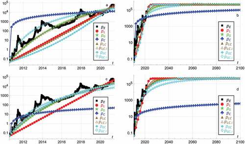
More specifically, section 3.1 estimates the Bitcoin price assuming no oscillation amplitude α = 0 and the Bitcoin carrying capacity K = $476,190 which corresponds to Bitcoin eventually approaching the market capitalization of gold estimated at $10 trillion. Section 3.2 repeats the exercise for the 50 times higher Bitcoin carrying capacity K = $23,809,524 which corresponds to Bitcoin eventually approaching a market capitalization of $500 trillion. Section 3.3 determines the three bull market local maxima and the three bear market local minima which have been established at the writing of this article. Section 3.4 estimates the scaling ω of the inverse of the cycle length of the sine oscillations and the scaling γ of the inverse of the degree of lengthening of each subsequent cycle. Section 3.5 allows for oscillation amplitude α ≥ 0 as determined by the previous two subsections, and estimates the Bitcoin price assuming the carrying capacity K = $476,190. Section 3.6 repeats the exercise for the 50 times higher Bitcoin carrying capacity K = $23,809,524. Section 3.7 estimates bull market local maxima 4,5,6,7,8 assuming the carrying capacities K = $476,190 and K = $23,809,524.

3.1. Bitcoin carrying capacity k=$476,190 and no oscillation amplitude α=0

The Bitcoin carrying capacity $K$ is estimated as the maximum sustainable market capitalization divided by the circulating supply. The Bitcoin circulating supply is capped at 21 million coins, expected to be mined by ca year 2140. Estimating Bitcoin’s maximum sustainable market capitalization is extremely uncertain. This section assumes that Bitcoin approaches a maximum sustainable market capitalization of $10 trillion, which is similar to the market capitalization of gold.¹ The comparison with gold is made since it would constitute a major milestone if Bitcoin were to reach it. Dividing $10 trillion with 21 million coins gives the Bitcoin carrying capacity $K=\mathrm{\$}476,190$. Using daily midnight 11:59.99 pm UTC closing time Bitcoin data,² the initial Bitcoin price at the initial time 23 July 2010 is $p_0=\mathrm{\$}0.04951$. Figure 1 shows the empirical price $p_E$ for the period 23 July 2010–21 June 2021, which increases overall, with intermittent decreases.³

Figure 1. Assuming no oscillation amplitude $\alpha =0$, the empirical price $p_E$, logistic growth $p_L$, Gompertz growth $p_G$, charged capacitor growth $p_C$, combined logistic and charged capacitor growth $p_{LC}$ and $p_{LC\lambda }$, and combined Gompertz and charged capacitor growth $p_{GC}$ and $p_{GC\lambda }$, for 23 July 2010–21 June 2021 (panels a and c) and until 1 January 2100 (panels b and d), $K=\mathrm{\$}476,190$. Panels a and b apply the least squares method. Panels c and d apply the weighted least squares method.

The subsequent seven curves in each panel in Figure 1 assume $\alpha =0$, $K=\mathrm{\$}476,190$ and $p_0=\mathrm{\$}0.04951$ and estimate the growth rate $k$, and the two parameters $\lambda$ and $\beta$, for the models in section 2.2. These seven curves increase strictly, in contrast to the empirical price $p_E$, due to the nature of growth models. In sections 3.5 and 3.6 oscillatory growth is modeled.

3.1.1. Least squares method

Applying the least squares method, Figure 1(a) shows the historical estimates. Figure 1(b) predicts until 1 January 2100. Using data over ca 11 years to predict ca 79 more years into the future, i.e., a ratio 79/11 ≈ 7.2, entails some uncertainty for the more distant future.

The curve $p_L$ estimates the growth rate $k=1.28$ by assuming logistic growth in (1) for $\nu =1$, approaching $K=\mathrm{\$}476,190$ more quickly than the other six curves. The curve $p_L$ appears almost linear on a logarithmic plot with base 10.

The curve $p_G$ estimates the growth rate $k=0.16$ by assuming Gompertz growth in (2). The curve $p_G$ is concave to reflect that the future value asymptote $t\to \mathrm{\infty }$ is approached more gradually than the initial value asymptote $t=t_0$. That is, initial growth is quick, and $K=\mathrm{\$}476,190$ is approached more slowly.

The curve $p_C$ estimates the growth rate $k=1178$ by assuming charged capacitor growth in (4). The curve $p_C$ is extremely concave. It initially increases more quickly than the other six curves, and eventually approaches $K=\mathrm{\$}476,190$ more slowly than the other six curves.

The curve $p_{LC}$ estimates the growth rate $k=1.21$ and adjustment parameter $\lambda =1.02$ by assuming combined logistic and charged capacitor growth in (6). Since $\lambda >1$, initial growth for the curve $p_{LC}$ is slower than for the curve $p_L$ for logistic growth, see section 2.4.

The curve $p_{LC\lambda }$ is intermediate between the curve $p_L$ for logistic growth and $p_C$ for charged capacitor growth. This is obtained by assuming $\lambda =0.88$ and using the least squares method to optimize the growth rate $k$ which gives $k=2.18$. The curve $p_{LC\lambda }$ is similar to Gompertz growth $p_G$.

The curve $p_{GC}$ estimates the growth rate $k=0.08$ and adjustment parameter $\lambda =1.17$ by assuming combined Gompertz and charged capacitor growth in (7). Since $\lambda >1$, initial growth for the curve $p_{GC}$ is slower than for the curve $p_G$ for Gompertz growth, see section 2.4.

The curve $p_{GC\lambda }$ is intermediate between the curve $p_G$ for Gompertz growth and $p_C$ for charged capacitor growth. This is obtained by assuming $\lambda =0.88$ and using the least squares method to optimize the growth rate $k$ which gives $k=0.32$. The curve $p_{GC\lambda }$ initially increases more quickly than all the other curves except the curve $p_C$ for charged capacitor growth.

3.1.2. Weighted least squares method

Applying the weighted least squares method, Figure 1(c) shows the historical estimates. Figure 1(d) predicts until 1 January 2100. The Bitcoin data exhibits heteroscedasticity so that the variance increases over time. That is, the Bitcoin price was $0.04951 on 23 July, 2010, with a few cents variation over the subsequent months until $1 was exceeded on 17 February 2011. In contrast, the Bitcoin price was $32,950 on 21 June 2021, with several thousand US$ variation over the preceding months until $1 was exceeded 17 February 2011. Hence the least squares method is more influenced by recent data than early data. This section assigns more weight to the earlier data by dividing each squared difference (between the model prediction and the data) at each time $t$ with the 20-week moving variance in the data, i.e., the variance over 140 days from time $t$ to time $t+139$. The variance calculation is constrained by the final time $T$ so that at time $T-1$ the variance over only the two final days at $T-1$ and $T$ is determined.

The two curves $p_L$ for logistic growth and $p_G$ for Gompertz growth have the same and slightly lower growth rates $k=1.28$ and $k=0.15$ as Figure 1(a) in section 3.1.1.

The curve $p_C$ for charged capacitor growth has the much lower growth rate $k=4.32$. That is because the early data is weighed more heavily, and more recent data is discounted. Hence the model prediction is worse for the more recent data, and the curve $p_C$ needs more time to approach the carrying capacity $K=\mathrm{\$}476,190$.

The curve $p_{LC}$ for combined logistic and charged capacitor growth estimates the higher growth rate $k=2.33$ and lower adjustment parameter $\lambda =0.85$, compared with Figure 1(a). Weighing the early data more heavily causes more rapid initial growth.

The curve $p_{LC\lambda }$ for combined logistic and charged capacitor growth when $\lambda =0.88$ has the lower growth rate $k=2.10$ compared with Figure 1(a), since it becomes less important to adjust to the recent data.

The curve $p_{GC}$ for combined Gompertz and charged capacitor growth estimates the higher growth rate $k=0.17$ and lower adjustment parameter $\lambda =0.97$, compared with Figure 1a. Weighing the early data more heavily causes more rapid initial growth.

The curve $p_{GC\lambda }$ for combined Gompertz and charged capacitor growth when $\lambda =0.88$ has the lower growth rate $k=0.22$ compared with Figure 1(a), since it becomes less important to adjust to the recent data.

3.2. Bitcoin carrying capacity K=$23,809,524 and no oscillation amplitude α=0

As an alternative, assume that Bitcoin in the future eradicates all or most other digital currencies, overtakes gold, bonds, and most other assets except physical real estate and various other physical assets. That may suggest a maximum sustainable market capitalization of $500 trillion, which may account for future inflation of the US$. Dividing $500 trillion with 21 million coins gives the Bitcoin carrying capacity $K=\mathrm{\$}23,809,524$. Figure 2 replicates Figure 1 for $K=\mathrm{\$}23,809,524$.

Figure 2. Assuming no oscillation amplitude $\alpha =0$, the empirical price $p_E$, logistic growth $p_L$, Gompertz growth $p_G$, charged capacitor growth $p_C$, combined logistic and charged capacitor growth $p_{LC}$ and $p_{LC\lambda }$, and combined Gompertz and charged capacitor growth $p_{GC}$ and $p_{GC\lambda }$, for 23 July 2010–21 June 2021 (panels a and c) and until 1 January 2100 (panels b and d), $K=\mathrm{\$}23,809,524$. Panels a and b apply the least squares method. Panels c and d apply the weighted least squares method.

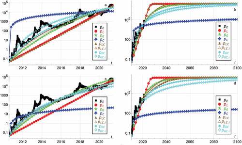
The subsequent seven curves in each panel in Figure 1 assume $\alpha =0$, $K=\mathrm{\$}23,809,524$ and $p_0=\mathrm{\$}0.04951$ and estimate the growth rate $k$, and the two parameters $\lambda$ and $\beta$, for the models in section 2.2, using the least squares method. Figure 1(a) shows the historical estimates. Figure 1(b) predicts until 1 January 2100.

3.2.1. Least squares method

Applying the least squares method, Figure 2(a) shows the historical estimates. Figure 2(b) predicts until 1 January 2100. Figure 2 gives similar parameter estimates to those in Figure 1.

The curve $p_L$ estimates slightly lower growth rate $k=1.27$ compared with Figure 1 for logistic growth in (1) for $\nu =1$.

The curve $p_G$ estimates lower growth rate $k=0.10$ compared with Figure 1 for Gompertz growth in (2).

The curve $p_C$ estimates slightly lower growth rate $k=1171$ compared with Figure 1 for charged capacitor growth in (4).

The curve $p_{LC}$ estimates slightly higher growth rate $k=1.23$ and slightly lower adjustment parameter $\lambda =1.01$, compared with Figure 1 for combined logistic and charged capacitor growth in (6).

The curve $p_{LC\lambda }$ estimates slightly lower growth rate $k=2.17$ when assuming the same adjustment parameter $\lambda =0.88$, compared with Figure 1 for combined logistic and charged capacitor growth in (6).

The curve $p_{GC}$ estimates higher growth rate $k=0.14$ and lower adjustment parameter $\lambda =0.94$ compared with Figure 1 for combined Gompertz and charged capacitor growth in (7).

The curve $p_{GC\lambda }$ estimates lower growth rate $k=0.20$ compared with Figure 1 when assuming adjustment parameter $\lambda =0.88$, for combined Gompertz and charged capacitor growth in (7).

3.2.2. Weighted least squares method

Applying the same weighted least squares method as in section 3.1.2, Figure 2(c) shows the historical estimates. Figure 2(d) predicts until 1 January 2100.

The two curves $p_L$ for logistic growth and $p_G$ for Gompertz growth have the same and slightly higher growth rates $k=1.28$ and $k=0.11$ compared with Figure 2(a) in section 3.2.1.

The curve $p_C$ for charged capacitor growth has the much lower growth rate $k=4.32$. That is because the early data is weighed more heavily, and more recent data is discounted. Hence the model prediction is worse for the more recent data, and the curve $p_C$ needs more time to approach the carrying capacity $K=\mathrm{\$}23,809,524$.

The curve $p_{LC}$ for combined logistic and charged capacitor growth estimates the higher growth rate $k=2.33$ and lower adjustment parameter $\lambda =0.85$, compared with Figure 2(a). Weighing the early data more heavily causes more rapid initial growth.

The curve $p_{LC\lambda }$ for combined logistic and charged capacitor growth when $\lambda =0.88$ has the lower growth rate $k=2.10$ compared with Figure 2(a), since it becomes less important to adjust to the recent data.

The curve $p_{GC}$ for combined Gompertz and charged capacitor growth estimates slightly lower growth rate $k=0.13$ and the same adjustment parameter $\lambda =0.94$, compared with Figure 2(a).

The curve $p_{GC\lambda }$ for combined Gompertz and charged capacitor growth when $\lambda =0.88$ has the lower growth rate $k=0.15$ compared with Figure 2(a), since it becomes less important to adjust to the recent data.

3.3. Determining the three bull market local maxima and the three bear market local minima

The three bull market local maxima since 23 July 2010, are as follows:

$29.6 on 14 June, 2011, expressed as $t_{1max}=2011.449315$, i.e., 327 days after the start date 23 July 2010 which is day 1.

$1131.992853 on 29 November, 2013 expressed as $t_{2max}=2013.909589$, i.e., 1226 days after the start date 23 July 2010 which is day 1.

$19,378.35059 on 16 December, 2017 expressed as $t_{3max}=2017.956164$, i.e., 2704 days after the start date 23 July 2010 which is day 1.

This gives 1226–327 = 899 days, i.e., 2.46027 years, from bull market local maximum 1 to bull market local maximum 2, and 2704–1226 = 1478 days, i.e., 4.04657 years, from bull market local maximum 2 to bull market local maximum 3.

The three bear market local minima since 23 July 2010 are as follows:

$2.2 on 20 November, 2011, expressed as $t_{1min}=2011.884932$, i.e., 486 days after the start date 23 July 2010 which is day 1.

$178.712075 on 14 January, 2015 expressed as $t_{2min}=2015.035616$, i.e., 1637 days after the start date 23 July 2010 which is day 1.

$3226.92952 on 14 December, 2018 expressed as $t_{3min}=2018.950685$, i.e., 3067 days after the start date 23 July 2010 which is day 1.

This gives 1637–486 = 1151 days, i.e., $3.15068$ years, from bear market local minimum 1 to bear market local minimum 2, and 3067–1637 = 1430 days, i.e., $3.915069$ years, from bear market local minimum 2 to bear market local minimum 3.

The modeling assumes oscillations in the sense that a maximum is followed by a minimum, then a new maximum, etc.

3.4. Estimating the scaling ω of the inverse of the cycle length of the sine oscillations and the scaling γ of the inverse of the degree of lengthening of each subsequent cycle

This section estimates the scaling $\omega$ of the inverse of the cycle length of the sine oscillations, and the scaling $\gamma$ of the inverse of the degree of lengthening of each subsequent cycle. The oscillatory growth rate with damped oscillation, retracement in bear markets, and lengthening cycles in all the equations in section 2 contain the sine of $\omega {\left(t-t_0\right)}^{\gamma }+\delta$. One cycle has time length $2\pi$. Hence the two equations

(8) $\left(\omega {\left(t_{2\mathrm{m}\mathrm{a}\mathrm{x}}-t_0\right)}^{\gamma }+\delta \right)-\left(\omega {\left(t_{1\mathrm{m}\mathrm{a}\mathrm{x}}-t_0\right)}^{\gamma }+\delta \right)=2\pi ,\left(\omega {\left(t_{3\mathrm{m}\mathrm{a}\mathrm{x}}-t_0\right)}^{\gamma }+\delta \right)-\left(\omega {\left(t_{2\mathrm{m}\mathrm{a}\mathrm{x}}-t_0\right)}^{\gamma }+\delta \right)=2\pi$(8)

express the time length from bull market local maximum 1 to bull market local maximum 2, and the time length from bull market local maximum 2 to bull market local maximum 3, respectively. Solving (8) by using $t_{1max}$, $t_{2max}$, $t_{3max}$ from section 3.3 gives ${\omega }_{max}=7.05885$ and ${\gamma }_{max}=0.499872$.

Analogously, the two equations

(9) $\left(\omega {\left(t_{2\mathrm{m}\mathrm{i}\mathrm{n}}-t_0\right)}^{\gamma }+\delta \right)-\left(\omega {\left(t_{1\mathrm{m}\mathrm{i}\mathrm{n}}-t_0\right)}^{\gamma }+\delta \right)=2\pi ,\left(\omega {\left(t_{3\mathrm{m}\mathrm{i}\mathrm{n}}-t_0\right)}^{\gamma }+\delta \right)-\left(\omega {\left(t_{2\mathrm{m}\mathrm{i}\mathrm{n}}-t_0\right)}^{\gamma }+\delta \right)=2\pi$(9)

express the time length from bear market local minimum 1 to bear market local minimum 2, and the time length from bear market local minimum 2 to bear market local minimum 3, respectively. Solving (9) by using $t_{1min}$, $t_{2min}$, $t_{3min}$ from section 3.3 gives ${\omega }_{min}=3.45348$ and ${\gamma }_{min}=0.744082$. The average of ${\omega }_{max}$ and ${\omega }_{min}$ is $\omega =5.25616$. The average of ${\gamma }_{max}$ and ${\gamma }_{min}$ is $\gamma =0.621977$.

3.5. Bitcoin carrying capacity K=$476,190 and oscillation amplitude α>0

This section assumes positive oscillation amplitude $\alpha \ge 0$ and assumes the same $k$, $\gamma$, and $\beta$ as when $\alpha =0$. Since $\omega =5.25616$ and $\gamma =0.621977$ are estimated in the previous section, we only have to estimate $\alpha$ and $\delta$. Figure 3 shows the empirical price $p_E$ for the period 23 July 2010–21 June 2021.

Figure 3. Assuming oscillation amplitude $\alpha \ge 0$, the empirical price $p_E$, logistic growth $p_L$, Gompertz growth $p_G$, charged capacitor growth $p_C$, combined logistic and charged capacitor growth $p_{LC}$ and $p_{LC\lambda }$, and combined Gompertz and charged capacitor growth $p_{GC}$ and $p_{GC\lambda }$, for 23 July 2010–21 June 2021 (panels a and c) and until 1 January 2040 (panels b and d), $K=\mathrm{\$}476,190$. Panels a and b apply the least squares method. Panels c and d apply the weighted least squares method.

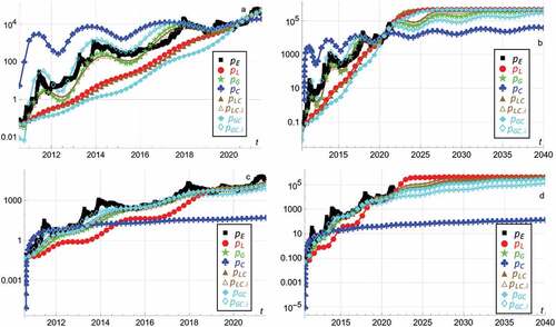
3.5.1. Least squares method

Applying the least squares method, Figure 3(a) shows the historical estimates. Figure 3(b) predicts until 1 January 2040.

The curve $p_L$ estimates the oscillation amplitude $\alpha =0.48$ and start time adjustment parameter $\delta =3.90$ for logistic growth in (1) for $\nu =1$ and $k=1.28$. The oscillation amplitude α is moderate relative to the almost linear curve in Figure 1.

The curve $p_G$ estimates the oscillation amplitude $\alpha =0.37$ and start time adjustment parameter $\delta =4.29$ for Gompertz growth in (2) when $k=0.16$. The oscillation amplitude α is higher than for the curve $p_L$, and conforms with the bull and bear markets.

The curve $p_C$ estimates the oscillation amplitude $\alpha =7209$ and start time adjustment parameter $\delta =5.03$ for charged capacitor growth in (4) when $k=1178$. The curve $p_C$ starts with extreme concavity, thereafter oscillates according to the bull and bear markets, and eventually approaches $K=\mathrm{\$}476,190$ slowly.

The curve $p_{LC}$ estimates the oscillation amplitude $\alpha =0.39$ and start time adjustment parameter $\delta =3.05$ for combined logistic and charged capacitor growth in (6) when $k=1.21$ and $\lambda =1.02$. The curve $p_{LC}$ oscillates similarly to Gompertz growth $p_G$.

The curve $p_{LC\lambda }$ estimates the oscillation amplitude $\alpha =3.93$ and start time adjustment parameter $\delta =4.12$ for combined logistic and charged capacitor growth in (6) when $k=2.18$ and $\lambda =0.88$. The curve $p_{LC\lambda }$ oscillates similarly to Gompertz growth $p_G$.

The curve $p_{GC}$ estimates the oscillation amplitude $\alpha =0.04$ and start time adjustment parameter $\delta =5.05$ for combined logistic and charged capacitor growth in (6) when $k=0.08$ and $\lambda =1.17$ . The curve $p_{GC}$ initially grows slower than all the other curves.

The curve $p_{GC\lambda }$ estimates the oscillation amplitude $\alpha =0.91$ and start time adjustment parameter $\delta =4.55$ for combined Gompertz and charged capacitor growth in (7) when $k=0.32$ and $\lambda =0.88$. The curve is intermediate between Gompertz growth $p_G$ and combined logistic and charged capacitor growth $p_{LC}$ on the one hand, and charged capacitor growth $p_C$ on the other hand. The curve $p_{GC}$ conforms with the bull and bear markets.

3.5.2. Weighted least squares method

Applying the weighted least squares method, Figure 3(c) shows the historical estimates. Figure 3(d) predicts until 1 January 2040.

The curve $p_L$ estimates the oscillation amplitude $\alpha =1.42$ and start time adjustment parameter $\delta =2.31$ for logistic growth in (1) for $\nu =1$ and $k=1.28$. The oscillation amplitude $\alpha$ is higher and the start time adjustment parameter $\delta$ is lower compared with Figure 3(a).

The curve $p_G$ estimates the oscillation amplitude $\alpha =0.08$ and start time adjustment parameter $\delta =2.48$ for Gompertz growth in (2) when $k=0.15$. Both the oscillation amplitude $\alpha$ and the start time adjustment parameter $\delta$ are lower compared with Figure 3(a).

The curve $p_C$ estimates the oscillation amplitude $\alpha =3.13$ and start time adjustment parameter $\delta =4.28$ for charged capacitor growth in (4) when $k=4.32$. The oscillation amplitude $\alpha$ is substantially lower, impacted by the much lower growth rate $k=4.32$, and the start time adjustment parameter $\delta$ is lower, compared with Figure 3(a). The curve $p_C$ eventually approaches $K=\mathrm{\$}476,190$ slowly.

The curve $p_{LC}$ estimates the oscillation amplitude $\alpha =1.88$ and start time adjustment parameter $\delta =3.24$ for combined logistic and charged capacitor growth in (6) when $k=2.33$ and $\lambda =0.85$. Both the oscillation amplitude $\alpha$ and the start time adjustment parameter $\delta$ are higher compared with Figure 3(a). The curve $p_{LC}$ oscillates similarly to Gompertz growth $p_G$.

The curve $p_{LC\lambda }$ estimates the oscillation amplitude $\alpha =1.65$ and start time adjustment parameter $\delta =3.02$ for combined logistic and charged capacitor growth in (6) when $k=2.10$ and $\lambda =0.88$. Both the oscillation amplitude $\alpha$ and the start time adjustment parameter $\delta$ are lower compared with Figure 3(a). The curve $p_{LC\lambda }$ also oscillates similarly to Gompertz growth $p_G$.

The curve $p_{GC}$ estimates the oscillation amplitude $\alpha =0.15$ and start time adjustment parameter $\delta =3.26$ for combined logistic and charged capacitor growth in (6) when $k=0.17$ and $\lambda =0.97$ . The oscillation amplitude $\alpha$ is higher and the start time adjustment parameter $\delta$ is lower compared with Figure 3(a). The curve $p_{GC}$ also oscillates similarly to Gompertz growth $p_G$.

The curve $p_{GC\lambda }$ estimates the oscillation amplitude $\alpha =0.20$ and start time adjustment parameter $\delta =3.93$ for combined Gompertz and charged capacitor growth in (7) when $k=0.22$ and $\lambda =0.88$. Both the oscillation amplitude $\alpha$ and the start time adjustment parameter $\delta$ are lower compared with Figure 3(a). The curve $p_{GC\lambda }$ initially oscillates around higher values than the other curves except charged capacitor growth $p_C$.

3.6. Bitcoin carrying capacity K=$23,809,524 and oscillation amplitude α>0

This section replicates the previous section with the higher Bitcoin carrying capacity $K=\mathrm{\$}23,809,524$. Figure 4 replicates Figure 3 for $K=\mathrm{\$}23,809,524$.

Figure 4. Assuming oscillations $\alpha \ge 0$, the empirical price $p_E$, logistic growth $p_L$, Gompertz growth $p_G$, charged capacitor growth $p_C$, combined logistic and charged capacitor growth $p_{LC}$ and $p_{LC\lambda }$, and combined Gompertz and charged capacitor growth $p_{GC}$ and $p_{GC\lambda }$, for 23 July 2010–21 June 2021 (panels a and c) and until 1 January 2040 (panels b and d), $K=\mathrm{\$}23,809,524$. Panels a and b apply the least squares method. Panels c and d apply the weighted least squares method.

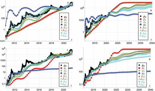
3.6.1. Least squares method

Applying the least squares method, Figure 4(a) shows the historical estimates. Figure 4(b) predicts until 1 January 2040. Figure (4) gives similar parameter estimates to those in Figure 3.

The curve $p_L$ estimates lower oscillation amplitude $\alpha =0.34$ and slightly higher start time adjustment parameter $\delta =4.00$ for logistic growth compared with Figure 3, assuming $\nu =1$ and $k=1.27$.

The curve $p_G$ estimates lower oscillation amplitude $\alpha =0.17$ and slightly higher start time adjustment parameter $\delta =4.34$ for Gompertz growth compared with Figure 3, assuming $k=0.10$.

The curve $p_C$ estimates slightly lower oscillation amplitude $\alpha =7200$ and slightly lower start time adjustment parameter $\delta =5.00$ for charged capacitor growth compared with Figure 3, assuming $k=1171$.

The curve $p_{LC}$ estimates lower oscillation amplitude $\alpha =0.22$ and higher start time adjustment parameter $\delta =3.69$ for combined logistic and charged capacitor growth compared with Figure 3, assuming $k=1.23$ and $\lambda =1.01$.

The curve $p_{LC\lambda }$ estimates lower oscillation amplitude $\alpha =3.58$ and lower start time adjustment parameter $\delta =4.08$ for combined logistic and charged capacitor growth compared with Figure 3, assuming $k=2.17$ and $\lambda =0.88$.

The curve $p_{GC}$ estimates substantially higher oscillation amplitude $\alpha =0.29$ and lower start time adjustment parameter $\delta =4.22$ for combined logistic and charged capacitor growth compared with Figure 3, assuming $k=0.14$ and $\lambda =0.94$.

The curve $p_{GC\lambda }$ estimates the same oscillation amplitude $\alpha =0.91$ and the same start time adjustment parameter $\delta =4.55$ for combined Gompertz and charged capacitor growth compared with Figure 3, assuming $k=0.2$ and $\lambda =0.88$.

3.6.2. Weighted least squares method

Applying the weighted least squares method, Figure 4(c) shows the historical estimates. Figure 4(d) predicts until 1 January 2040.

The curve $p_L$ estimates substantially higher oscillation amplitude $\alpha =1.53$ and lower start time adjustment parameter $\delta =2.38$ compared with Figure 4(a) for logistic growth, assuming $\nu =1$ and $k=1.27$ as in Figure 2.

The curve $p_G$ estimates lower oscillation amplitude $\alpha =0.11$ and lower start time adjustment parameter $\delta =3.40$ compared with Figure 4(a) for Gompertz growth, assuming $k=0.11$ as in Figure 2.

The curve $p_C$ estimates substantially lower oscillation amplitude $\alpha =3.13$ and lower start time adjustment parameter $\delta =4.28$ compared with Figure 4(a) for charged capacitor growth, assuming $k=4.32$ as in Figure 2. The difference between Figure 4(c) and Figure 4(a) is similar to the difference between Figure 2(c) and Figure 2(a).

The curve $p_{LC}$ estimates substantially higher oscillation amplitude $\alpha =1.66$ and lower start time adjustment parameter $\delta =3.23$ compared with Figure 4(a) for combined logistic and charged capacitor growth, assuming $k=2.33$ and $\lambda =0.85$ as in Figure (2).

The curve $p_{LC\lambda }$ estimates lower oscillation amplitude $\alpha =1.65$ and lower start time adjustment parameter $\delta =3.00$ compared with Figure 4(a) for combined logistic and charged capacitor growth, assuming $k=2.10$ and $\lambda =0.88$ as in Figure 2.

The curve $p_{GC}$ estimates lower oscillation amplitude $\alpha =0.15$ and start time adjustment parameter $\delta =3.5$ compared with Figure 4(a) for combined logistic and charged capacitor growth, assuming $k=0.13$ and $\lambda =0.94$ as in Figure 2.

The curve $p_{GC\lambda }$ estimates the much lower oscillation amplitude $\alpha =0.20$ and lower start time adjustment parameter $\delta =3.93$ compared with Figure 4(a) for combined Gompertz and charged capacitor growth, assuming $k=0.15$ and $\lambda =0.88$ as in Figure 2.

3.7. Estimating bull market local maxima 4,5,6,7,8 when K=$476,190 and K=$23,809,524

Table 1 predicts the dates and magnitudes of the five future Bitcoin bull market local price maxima, assuming $K=\mathrm{\$}476,190$ and $K=\mathrm{\$}23,809,524$, and assuming logistic growth $p_L$, Gompertz growth $p_G$, charged capacitor growth $p_C$, combined logistic and charged capacitor growth $p_{LC}$ and $p_{LC\lambda }$, and combined Gompertz and charged capacitor growth $p_{GC}$ and $p_{GC\lambda }$.

Table 1. Dates and magnitudes of bull market local maxima 4,5,6,7,8 when $K=\mathrm{\$}476,190$ and $K=\mathrm{\$}23,809,524$, predicted until year 2050

Bull market local maximum	4	5	6	7	8
Logistic growth $p_L$	Asymptotic. 07/06/24; 431,785. Asymptotic. 05/05/24; 3,360,314.	Asymptotic. 01/28/30; 476,153. Asymptotic. 11/18/29; 23,694,323.	Asymptotic. Asymptotic. Asymptotic. 02/06/36; 23,809,485.	Asymptotic. Asymptotic. Asymptotic. Asymptotic.	Asymptotic. Asymptotic. Asymptotic. Asymptotic.
Gompertz growth $p_G$	05/22/22; 75,506. Asymptotic. 06/29/22; 107,064. Asymptotic.	08/25/27; 221,873. Asymptotic. 10/08/27; 1,032,330. Asymptotic.	08/11/33; 358,456. Asymptotic. 09/29/33; 4,343,140. Asymptotic.	03/21/40; 432,860. Asymptotic. 05/15/40; 10,021,700. Asymptotic.	06/11/47; 462,526. Asymptotic. 08/09/47; 15,732,787. Asymptotic.
Charged capacitor growth $p_C$	08/08/21; 18,032. Asymptotic. 08/15/21; 18,317. Asymptotic.	09/29/26; 24,619. Asymptotic. 10/07/26; 25,173. Asymptotic.	08/05/32; 31,829. Asymptotic. 08/14/32; 32,789. Asymptotic.	02/07/39; 39,587. Asymptotic. 02/17/39; 41,119. Asymptotic.	03/25/46; 47,827. Asymptotic. 04/04/46; 50,127. Asymptotic.
Combined logistic and charged capacitor growth $p_{LC}$	Asymptotic. Asymptotic. Asymptotic. Asymptotic.	Asymptotic. Asymptotic. Asymptotic. Asymptotic.	Asymptotic. Asymptotic. Asymptotic. Asymptotic.	Asymptotic. Asymptotic. Asymptotic. Asymptotic.	Asymptotic. Asymptotic. Asymptotic. Asymptotic.
Combined logistic and charged capacitor growth $p_{LC\lambda }$	08/19/22; 113,012. Asymptotic. 09/16/22; 133,710. Asymptotic.	12/05/27; 391,125. Asymptotic. 01/07/28; 1,497,123. Asymptotic.	12/03/33; 470,084. Asymptotic. 01/08/34; 8,753,549. Asymptotic.	07/25/40; 475,908. Asymptotic. 09/03/40; 19,460,471. Asymptotic.	10/26/47; 476,180. Asymptotic. 12/08/47; 23,181,174. Asymptotic.
Combined Gompertz and charged capacitor growth $p_{GC}$	Asymptotic. Asymptotic. 06/26/22; 94,049. 06/27/23; 65,062.	Asymptotic. Asymptotic. 10/05/27; 512,728. 11/27/28; 367,353.	Asymptotic. Asymptotic. 09/25/33; 1,714,019. 01/06/35; 1,286,048.	Asymptotic. Asymptotic. 05/10/40; 4,022,084. 10/06/41; 3,169,232.	Asymptotic. Asymptotic. 08/04/47; 7,301,533. 02/12/49; 6,030,620.
Combined Gompertz and charged capacitor growth $p_{GC\lambda }$	02/12/22; 46,652. Asymptotic. 04/28/22; 68,116. Asymptotic.	05/03/27; 110,018. Asymptotic. 07/29/27; 264,925. Asymptotic.	04/05/33; 191,648. Asymptotic. 07/11/33; 736,127. Asymptotic.	11/02/39; 273,762. Asymptotic. 02/16/40; 1,611,829. Asymptotic.	01/10/47; 342,930. Asymptotic. 05/06/47; 2,960,784. Asymptotic.
Date and local maximum expected value $\pm$ standard deviation	12/12/22 $\pm 314$. 11/29/22 $\pm 397$. 05/18/22 $\pm$ 94. 07/06/24 $\pm 0$. 12/21/22 $\pm$ 288. 07/02/22 $\pm 58$. 11/30/23 $\pm$ 221. 166,739 $\pm$ 178,774. 78,390 $\pm 33,274$. 431,785 $\pm 0$. 638,053 $\pm 1,333,874$. 100,735 $\pm 27,301$. 1,712,688 $\pm 2,330,095.$	04/15/28 $\pm 359$. 03/30/28 $\pm 454$. 08/21/27 $\pm$ 108. 01/28/30 $\pm 0$. 04/25/28 $\pm$ 329. 10/12/27 $\pm 66$. 05/24/29 $\pm$ 252. 299,792 $\pm$ 164,854. 241,005 $\pm 141,527$. 476,153 $\pm 0$. 4,561,464 $\pm 9,384,608$. 826,777 $\pm 549,521$. 12,030,838 $\pm 16,494,659.$	02/07/34 $\pm 327$. 08/06/33 $\pm 121$. 08/06/33 $\pm 121$. Asymptotic. 05/10/34 $\pm 367$. 10/03/33 $\pm 74$. 07/23/35 $\pm 280$. 340,063 $\pm 140,126$. 340,063 $\pm 140,126$. Asymptotic. 6,773,728 $\pm 8,856,776$. 3,886,709 $\pm 3,584,281$. 12,547,767 $\pm 15,926,475.$	06/27/40 $\pm 211$. 03/16/40 $\pm 133$. 03/16/40 $\pm 133$. Asymptotic. 08/28/40 $\pm 237$. 05/19/40 $\pm 82$. 10/06/41 $\pm 0$. 394,177 $\pm 106,480$. 394,177 $\pm 106,480$. Asymptotic. 7,657,063 $\pm 7,328,208$. 8,779,021 $\pm 7,950,571$. 3,169,232 $\pm 0.$	09/25/47 $\pm 228$. 06/06/47 $\pm 145$. 06/06/47 $\pm 145$. Asymptotic. 12/01/47 $\pm 257$. 08/14/47 $\pm 89$. 02/12/49 $\pm 0$. 427,212 $\pm 73,309$. 427,212 $\pm 73,309$. Asymptotic. 11,041,380 $\pm 8,273,060$. 12,294,070 $\pm 8,988,687$. 6,030,620 $\pm 0$.

Each cell has four entries, except in the bottom row. Each entry ends with period ”.”. The dates are in the format month/day/year for the least squares method and the weighted least squares method in entries 1 and 2 when $K=\mathrm{\$}476,190$. Entries 3 and 4 are for the least squares method and the weighted least squares method when $K=\mathrm{\$}23,809,524$. After each date the price follows in $. Asymptotic means that no local maximum exists, but that the Bitcoin price $p$ approaches $K$ asymptotically. In the bottom row each cell has 13 entries. Each entry ends with period ”.”. This gives seven entries with dates and six entries with local maxima expressed as expected value $\pm$ standard deviation in days and $\mathrm{\$}$. Entry 1 gives the date for both methods and both $K=\mathrm{\$}476,190$ and $K=\mathrm{\$}23,809,524$. Entries 2 and 8 apply for both methods when $K=\mathrm{\$}476,190$. Entries 3 and 9 apply for the least squares method when $K=\mathrm{\$}476,190$. Entries 4 and 10 apply for the weighted least squares method when $K=\mathrm{\$}476,190$. Entries 5 and 11 apply for both methods when $K=\mathrm{\$}23,809,524$. Entries 6 and 12 apply for the least squares method when $K=\mathrm{\$}23,809,524$. Entries 7 and 13 apply for the weighted least squares method when $K=\mathrm{\$}23,809,524$.

Table 2 analogously predicts the dates and magnitudes of the five future Bitcoin bear market local price minima, assuming $K=\mathrm{\$}476,190$ and $K=\mathrm{\$}23,809,524$, and assuming logistic growth $p_L$, Gompertz growth $p_G$, charged capacitor growth $p_C$, combined logistic and charged capacitor growth $p_{LC}$ and $p_{LC\lambda }$, and combined Gompertz and charged capacitor growth $p_{GC}$ and $p_{GC\lambda }$.

Table 2. Dates and magnitudes of bear market local minima 4,5,6,7,8 when $K=\mathrm{\$}476,190$ and $K=\mathrm{\$}23,809,524$, predicted until year 2050

Bear market local minima	4	5	6	7	8
Logistic growth $p_L$	Asymptotic. 04/09/25; 428,795. Asymptotic. 05/01/25; 2,898,043.	Asymptotic. 12/07/30; 476,150. Asymptotic. 01/01/31; 23,669,932.	Asymptotic. Asymptotic. Asymptotic. 05/05/37; 23,809,475.	Asymptotic. Asymptotic. Asymptotic. Asymptotic.	Asymptotic. Asymptotic. Asymptotic. Asymptotic.
Gompertz growth $p_G$	03/05/24; 45,736. Asymptotic. 12/28/23; 73,350. Asymptotic.	09/10/29; 174,196. Asymptotic. 06/24/29; 802,142. Asymptotic.	11/22/35; 323,674. Asymptotic. 08/27/35; 3,725,750. Asymptotic.	09/22/42; 416,631. Asymptotic. 06/19/42; 9,196,504. Asymptotic.	02/27/50; 456,629. Asymptotic. 11/16/49; 15,043,891. Asymptotic.
Charged capacitor growth $p_C$	10/24/23; 9,710. Asymptotic. 11/01/23; 9,743. Asymptotic.	04/12/29; 15,198. Asymptotic. 04/21/29; 15,342. Asymptotic.	06/07/35; 21,449. Asymptotic. 06/16/35; 21,799. Asymptotic.	03/21/42; 28,365. Asymptotic. 04/01/42; 29,046. Asymptotic.	08/11/49; 35,866. Asymptotic. 08/22/49; 37,031. Asymptotic.
Combined logistic and charged capacitor growth $p_{LC}$	Asymptotic. Asymptotic. Asymptotic. Asymptotic.	Asymptotic. Asymptotic. Asymptotic. Asymptotic.	Asymptotic. Asymptotic. Asymptotic. Asymptotic.	Asymptotic. Asymptotic. Asymptotic. Asymptotic.	Asymptotic. Asymptotic. Asymptotic. Asymptotic.
Combined logistic and charged capacitor growth $p_{LC\lambda }$	03/17/24; 78,327. Asymptotic. 03/09/24; 95,424. Asymptotic.	09/24/29; 355,689. Asymptotic. 09/14/29; 1,139,873. Asymptotic.	12/07/35; 466,389. Asymptotic. 11/27/35; 7,376,641. Asymptotic.	10/08/42; 475,712. Asymptotic. 09/27/42; 18,476,294. Asymptotic.	03/16/50; 476,173. Asymptotic. 03/04/50; 22,992,469. Asymptotic.
Combined Gompertz and charged capacitor growth $p_{GC}$	Asymptotic. Asymptotic. 03/11/24; 57,377. 05/03/24; 62,860.	Asymptotic. Asymptotic. 09/17/29; 360,351. 11/16/29; 358,295.	Asymptotic. Asymptotic. 11/29/35; 1,334,243. 02/04/36; 1,263,066.	Asymptotic. Asymptotic. 09/30/42; 3,371,727. 12/12/42; 3,128,527.	Asymptotic. Asymptotic. 03/07/50; 6,458,819. 05/25/50; 5,975,591.
Combined Gompertz and charged capacitor growth $p_{GC\lambda }$	01/17/24; 27,008. Asymptotic. 01/14/24; 45,585. Asymptotic.	07/18/29; 77,314. Asymptotic. 07/13/29; 196,739. Asymptotic.	09/22/35; 152,541. Asymptotic. 09/18/35; 587,238. Asymptotic.	07/17/42; 236,548. Asymptotic. 07/12/42; 1,354,016. Asymptotic.	12/16/49; 312,871. Asymptotic. 12/11/49; 2,585,103. Asymptotic.
Date and local minima expected value $\pm$ standard deviation	05/17/24 $\pm 182$. 06/04/24 $\pm 208$. 02/22/24 $\pm$ 32. 04/09/25 $\pm 0$. 05/06/24 $\pm$ 182. 02/06/24 $\pm 38$. 10/31/24 $\pm$ 257. 144,966 $\pm$ 190,403. 50,357 $\pm 25,970$. 428,795 $\pm 0$. 538,773 $\pm 1,155,924$. 67,934 $\pm 21,571$. 1,480,452 $\pm 2,004,777$.	12/02/29 $\pm 206$. 12/22/29 $\pm 235$. 08/27/29 $\pm 36$. 12/07/30 $\pm 0$. 11/18/29 $\pm$ 207. 08/09/29 $\pm 43$. 06/09/30 $\pm$ 291. 270,837 $\pm$ 179,019. 202,400 $\pm 141,314$. 476,150 $\pm 0$. 4,421,222 $\pm 9,436,336$. 624,776 $\pm 428,143$. 12,014,113 $\pm 16,483,817$.	01/07/36 $\pm 188$. 11/06/35 $\pm 40$. 11/06/35 $\pm 40$. Asymptotic. 02/07/36 $\pm 229$. 10/18/35 $\pm 48$. 09/19/36 $\pm 322$. 314,201 $\pm 157,138$. 314,201 $\pm 157,138$. Asymptotic. 6,349,402 $\pm 8,910,871$. 3,255,968 $\pm 3,055,912$. 12,536,271 $\pm 15,942,719$.	09/06/42 $\pm 58$. 09/05/42 $\pm 44$. 09/05/42 $\pm 44$. Asymptotic. 09/07/42 $\pm 70$. 08/14/42 $\pm 53$. 12/12/42 $\pm 0$. 376,297 $\pm 124,579$. 376,297 $\pm 124,579$. Asymptotic. 7,105,414 $\pm 7,008,998$. 8,099,635 $\pm 7,675,386$. 3,128,527 $\pm 0$.	02/09/50 $\pm 63$. 02/08/50 $\pm 48$. 02/08/50 $\pm 48$. Asymptotic. 02/10/50 $\pm 76$. 01/16/50 $\pm 57$. 05/25/50 $\pm 0$. 415,224 $\pm 89,177$. 415,224 $\pm 89,177$. Asymptotic. 10,611,175 $\pm 8,308,037$. 11,770,071 $\pm 9,114,698$. 5,975,591 $\pm 0$.

The structure is the same as for Table 1, but applies for local minima instead of local maxima.

3.7.1. Bitcoin carrying capacity K=$476,190

Assuming the Bitcoin carrying capacity $K=\mathrm{\$}476,190$, for logistic growth $p_L$ no local maxima exist with the least squares method, which means that the Bitcoin price $p$ increases monotonically and asymptotically towards $K=\mathrm{\$}476,190$ with no local maxima. The absence of local maxima is due to logistic growth $p_L$ approaching $K=\mathrm{\$}476,190$ more quickly than the other six curves (see Figure 1), and also due to logistic growth $p_L$ exhibiting limited oscillation, thus not tracking the empirics very well. Two local maxima exist with the weighted least squares method, after which the Bitcoin price $p$ increases monotonically towards $K=\mathrm{\$}476,190$. The presence of two local maxima is intermediate between no local maxima and five local maxima, reflecting more oscillation due to more weight being assigned to the early data, and better tracking of the early empirics. Since logistic growth $p_L$ approaches $K=\mathrm{\$}476,190$ more quickly than the other six curves, both local maxima are above $431,785, at 7/6/24 and 1/28/30.

For Gompertz growth $p_G$, five local maxima exist with the least squares method, starting with $75,506 at 5/22/22, and ending with $462,526 at 6/11/47. These lower local maxima, compared with logistic growth $p_L$, arise since Gompertz growth $p_G$ approaches the Bitcoin carrying capacity $K=\mathrm{\$}476,190$ more slowly. No local maxima exist with the weighted least squares method, reflecting less oscillation than with the least squares method.

For charged capacitor growth $p_C$ five local maxima exist with the least squares method. Since charged capacitor growth $p_C$ approaches the Bitcoin carrying capacity $K=\mathrm{\$}476,190$ slowly (see Figure 1), the local maxima are low, ranging from $18,032 at 8/8/21 to $47,827 at 3/25/46. No local maxima exist with the weighted least squares method, reflecting the much lower growth rate $k=4.32$, and inability to track the empirical oscillations.

For combined logistic and charged capacitor growth $p_{LC}$, no local maxima exist with the least squares method and the weighted least squares method. This result is influenced by no local maxima existing for logistic growth $p_L$ with the least squares method, and no local maxima existing for charged capacitor growth $p_C$ with the weighted least squares method.

For combined logistic and charged capacitor growth $p_{LC\lambda }$, five local maxima exist with the least squares method, starting with $113,012 at 8/19/22, and ending with $476,180 at 10/26/47. No local maxima exist with the weighted least squares method, reflecting less oscillation.

For combined Gompertz and charged capacitor growth $p_{GC}$, no local maxima exist with the least squares method and the weighted least squares method, due to less oscillation.

For combined Gompertz and charged capacitor growth $p_{GC\lambda }$, five local maxima exist with the least squares method, starting with $46,652 at 2/12/22, and ending with $342,930 at 1/10/47. No local maxima exist with the weighted least squares method, reflecting less oscillation.

3.7.2. Bitcoin carrying capacity K=$23,809,524

Assuming the Bitcoin carrying capacity $K=\mathrm{\$}23,809,524$, the results are remarkably similar to when $K=\mathrm{\$}476,190$. The local maxima mostly occur at the similar time $t$, but are naturally higher. For logistic growth $p_L$, no local maxima exist with the least squares method, while three local maxima exist with the weighted least squares method. These range from $3,360,314 at 5/5/24 to $23,809,485 at 2/6/36.

For Gompertz growth $p_G$ the five local maxima with the least squares method range from $107,064 at 6/29/22 to $15,732,787 at 8/9/47, i.e., lower than for logistic growth $p_L$. No local maxima exist with the weighted least squares method.

For charged capacitor growth $p_C$ the five local maxima with the least squares method only slightly exceed the local maxima when $K=\mathrm{\$}476,190$, and almost at the same time, ranging from $18,317 at 8/15/21 to $50,127 at 4/4/46. No local maxima exist with the weighted least squares method.

For combined logistic and charged capacitor growth $p_{LC}$, no local maxima exist with the least squares method and the weighted least squares method.

For combined logistic and charged capacitor growth $p_{LC\lambda }$, five local maxima exist with the least squares method, starting with $133,710 at 9/16/22, and ending with $23,181,174 at 12/8/47. No local maxima exist with the weighted least squares method.

For combined Gompertz and charged capacitor growth $p_{GC}$, local maxima exist with both the least squares method and the weighted least squares method, contrary to when $K=\mathrm{\$}476,190$. With the least squares method the five local maxima range from $94,049 at 6/26/22 to $7,301,533 at 8/4/47. With the weighted least squares method the five local maxima range from the lower $65,062 at 6/26/22 to the lower $6,030,620 at 2/12/49.

For combined Gompertz and charged capacitor growth $p_{GC\lambda }$, five local maxima exist with the least squares method, starting with $68,116 at 4/28/22, and ending with $2,960,784 at 5/6/47. No local maxima exist with the weighted least squares method.

4. Discussion

Ten results in the previous section are noteworthy. First, based on the current market capitalization of gold at approximately $10 trillion, the Bitcoin carrying capacity is estimated as $K=\mathrm{\$}476,190$. Using the least squares method, without modeling oscillations, logistic growth $p_L$ appears nearly linear with growth rate $k=1.28$ on a logarithmic plot with base 10. It initially increases more slowly, and eventually approaches $K=\mathrm{\$}476,190$ more quickly. Gompertz growth $p_G$ with growth rate $k=0.16$ is fast at the beginning and approaches $K=\mathrm{\$}476,190$ slowly. Charged capacitor growth $p_C$ initially grows much faster than the other six curves, with growth rate $k=1178$, and approaches $K=\mathrm{\$}476,190$ much slower than the other six curves. Combined logistic and charged capacitor growth $p_{LC}$ is slower than logistic growth $p_L$ but faster than combined Gompertz and charged capacitor growth $p_{GC}$. The curve $p_{LC}$ estimates the growth rate $k=1.21$ and adjustment parameter $\lambda =1.02$. Assuming $\lambda =0.88,$ the curve $p_{LC\lambda }$ with growth rate $k=2.18$ is intermediate between $p_L$ for logistic growth and $p_C$ for charged capacitor growth. Combined Gompertz and charged capacitor growth $p_{GC}$ displays initial slow growth rate $k=0.08$, but eventually approaches $K=\mathrm{\$}476,190$ quickly. Assuming $\lambda =0.88,$ the curve $p_{GC\lambda }$ with growth rate $k=0.32$ is intermediate between $p_G$ for Gompertz growth and $p_C$ for charged capacitor growth, and grows as the second fastest among the six curves. Summing up impressionistically, the curves $p_{GC\lambda }$, $p_{LC\lambda }$ and $p_G$ in Figure 1(a) fit the data relatively well.

Second, applying the weighted least squares method when $K=\mathrm{\$}476,190$, early data (with low price fluctuations measured in US$) is weighed more heavily than late data (with high price fluctuations measured in US$), which eliminates or ameliorates the impact of heteroscedasticity since more equal weight is assigned over the period 23 July 2010–21 June 2021, causing some similar and some different results. Logistic growth $p_L$ estimates the same growth rate $k=1.28$. Gompertz growth $p_G$ has the higher growth rate $k=0.15$. Charged capacitor growth $p_C$ has the much lower growth rate $k=4.32$, and approaches $K=\mathrm{\$}476,190$ more slowly than with the least squares method. Combined logistic and charged capacitor growth $p_{LC}$ has higher growth rate $k=2.33$ and lower adjustment parameter $\lambda =0.85$. Assuming $\lambda =0.88$, the curve $p_{LC\lambda }$ estimates the lower growth rate $k=2.10$. Combined Gompertz and charged capacitor growth $p_{GC}$ has higher growth rate $k=0.17$ and lower adjustment parameter $\lambda =0.97$. Assuming $\lambda =0.88,$ the curve $p_{GC\lambda }$ has lower growth rate $k=0.22$. Summing up, the curves $p_G,$ $p_{GC}$, $p_{GC\lambda }$, $p_{LC}$ and $p_{LC\lambda }$ in Figure 1(c) are relatively similar with seemingly good fit to the data.

Third, based on a Bitcoin market capitalization of $500 trillion, the Bitcoin carrying capacity is estimated as $K=\mathrm{\$}23,809,524$, i.e., 50 times higher than $K=\mathrm{\$}476,190$. The results and especially the dates of the local maxima are similar, but the local maxima are higher. Using the least squares method, without modeling oscillations, logistic growth $p_L$ is slightly lower at $k=1.27$. Gompertz growth $p_G$ is lower at $k=0.10$. Charged capacitor growth $p_C$ is slightly lower at $k=1171$. Combined logistic and charged capacitor growth $p_{LC}$ and $p_{LC\lambda }$ are similar at $k=1.23$ and $k=2.17$. Combined Gompertz and charged capacitor growth $p_{GC}$ and $p_{GC\lambda }$ (assuming $\lambda =0.88$) are higher at $k=0.14$ and lower at $k=0.20$, respectively. Summing up, the curves $p_G$, $p_{GC}$, $p_{LC\lambda }$, $p_{GC\lambda }$ in Figure 2(a) seem to fit the data well.

Fourth, applying the weighted least squares method when $K=\mathrm{\$}23,809,524$, logistic growth $p_L$ and Gompertz growth $p_G$ are similar at $k=1.27$ and $k=0.11$. Charged capacitor growth $p_C$ is much lower than with the least squares method, at $k=4.32$ (due to weighing early data more heavily). Combined logistic and charged capacitor growth $p_{LC}$ and $p_{LC\lambda }$ are higher at $k=2.33$ and lower at $k=2.10$, respectively. Combined Gompertz and charged capacitor growth $p_{GC}$ and $p_{GC\lambda }$ are slightly lower at $k=0.13$ and lower at $k=0.15$, respectively. Summing up, the curves $p_G$, $p_{GC}$, $p_{LC}$, $p_{LC\lambda }$, $p_{GC\lambda }$ in Figure 2(c) seem to fit the data well.

Fifth, the three bull market local maxima during the period 23 July 2010–21 June 2021 are used to estimate the scaling of the inverse of the cycle length of the sine oscillations as ${\omega }_{max}=7.05885$, and the inverse of the degree of lengthening of each subsequent cycle as ${\gamma }_{max}=0.499872$. The three bear market local minima during the period 23 July 2010–21 June 2021 are analogously used to estimate ${\omega }_{min}=3.45348$ and ${\gamma }_{min}=0.744082$. Taking the average, $\omega =5.25616$ as the scaling of the inverse of the cycle length of the sine oscillations, and $\gamma =0.621977$ as the inverse of the degree of lengthening of each subsequent cycle, are used in the remainder of the article.

Sixth, applying the same growth rate $k$ and adjustment parameter $\lambda$ as estimated without assuming oscillations (i.e., when $\alpha =0$), and applying $\omega =5.25616$ and $\gamma =0.621977$, the oscillation amplitude $\alpha$ and the start time adjustment parameter $\delta$ are estimated to model oscillatory growth for the models. With Bitcoin carrying capacity $K=\mathrm{\$}476,190$ and applying the least squares method, logistic growth $p_L$ oscillates minimally at the amplitude $\alpha =0.48$. Gompertz growth $p_G$ oscillates more at $\alpha =0.37$. Charged capacitor growth $p_C$ oscillates moderately at $\alpha =7209$. Combined logistic and charged capacitor growth $p_{LC}$ oscillates similarly to logistic growth $p_L$ at $\alpha =0.39$. The curve $p_{LC\lambda }$ oscillates similarly to Gompertz growth $p_G$ at $\alpha =3.93$. Combined Gompertz and charged capacitor growth $p_{GC}$ oscillates minimally at $\alpha =0.04$. The curve $p_{GC\lambda }$ oscillates at $\alpha =0.91$. Summing up, the curves $p_G$, $p_{GC}$, $p_{LC\lambda }$, $p_{GC\lambda }$ in Figure 3(a) seemingly oscillate nicely according to the data.

Seventh, applying the weighted least squares method when $K=\mathrm{\$}476,190$, logistic growth $p_L$ oscillates more at $\alpha =1.42$. Gompertz growth $p_G$ oscillates less at $\alpha =0.08$. Charged capacitor growth $p_C$ oscillates minimally at $\alpha =3.13$. Combined logistic and charged capacitor growth $p_{LC}$ and $p_{LC\lambda }$ oscillate similarly to Gompertz growth $p_G$ at $\alpha =1.88$ and $\alpha =1.65$. Combined Gompertz and charged capacitor growth $p_{GC}$ oscillates at $\alpha =0.15$. The curve $p_{GC\lambda }$ oscillates at $\alpha =0.20$. Summing up, the curves $p_G$, $p_{GC}$, $p_{LC}$, $p_{LC\lambda }$, $p_{GC\lambda }$ in Figure 3(c) seem to oscillate according to the data.

Eighth, with Bitcoin carrying capacity $K=\mathrm{\$}23,809,524$ and applying the least squares method, logistic growth $p_L$ and combined logistic and charged capacitor growth $p_{LC}$ oscillate similarly and minimally at $\alpha =0.34$ and $\alpha =0.22$. Gompertz growth $p_G$ oscillates at $\alpha =0.17$. Charged capacitor growth $p_C$ oscillates moderately at $\alpha =7200$. The curve $p_{LC\lambda }$ oscillates similarly to Gompertz growth $p_G$ at $\alpha =3.58$. Combined Gompertz and charged capacitor $p_{GC}$ oscillates at $\alpha =0.29$. The curve $p_{GC\lambda }$ oscillates at $\alpha =0.91$. Summing up, the curves $p_G$, $p_{GC}$, $p_{LC\lambda }$, $p_{GC\lambda }$ in Figure 4(a) seemingly oscillate according to the data.

Ninth, applying the weighted least squares method when $K=\mathrm{\$}23,809,524$, logistic growth $p_L$ again oscillates more at $\alpha =1.53$. Gompertz growth $p_G$ and combined logistic and charged capacitor growth $p_{LC}$ and $p_{LC\lambda }$ oscillate similarly at $\alpha =0.11$, $\alpha =1.66$, and $\alpha =1.65$. Charged capacitor growth $p_C$ oscillates at $\alpha =3.13$. Combined Gompertz and charged capacitor growth $p_{GC}$ and $p_{GC\lambda }$ oscillate at $\alpha =0.15$ and $\alpha =0.20$. Summing up, the curves $p_G$, $p_{GC}$, $p_{LC}$, $p_{LC\lambda }$, $p_{GC\lambda }$ in Figure 4(c) seem to oscillate according to the data.

Tenth, applying the two Bitcoin carrying capacities $K=\mathrm{\$}476,190$ and $K=\mathrm{\$}23,809,524$, the bull market local maxima 4,5,6,7,8 and bear market local minima 4,5,6,7,8 are estimated until 2050. These dates depend to a low degree on the growth model carrying capacity $K$. The magnitudes of the local maxima and local minima of course depend on $K$, assumed to vary broadly to assess the implications.

If the Bitcoin price evolves until the year 2100 as predicted in this article, that has substantial implications for today’s financial system. First, Bitcoin may become a more dominant investment class competing with today’s classes, i.e., stocks, bonds, real estate, money market instruments, non-inflationary instruments (minerals, art, etc.), etc. Second, if Bitcoin layer 2 solutions become common, as in El Salvador, such solutions may spread to more countries, and likely first to the world’s countries with the weakest currencies or countries without their own currency. The insights in this article may be useful for all humans, i.e., consumers choosing between Bitcoin layer 2 solutions and alternative payment rails, investors, politicians and regulators choosing how to regulate Bitcoin, regulators and developers of asset classes competing with Bitcoin, financial institutions competing with Bitcoin or developing Bitcoin-based instruments, and central banks developing digital currencies.

5. Conclusion

The motivation for this article is the apparently unpredictable Bitcoin price evolution since 3 January 2009, and the need for methods to understand the evolution so far and predict the future evolution. The methods are differential equation growth models incorporating oscillation and lengthening cycles. The analysis is interesting for traders (with time horizons from microseconds to months or years) exchanging Bitcoin with other cryptocurrencies, fiat currencies and asset classes, and savers and investors choosing Bitcoin as a mid term or long term store of value. The article is also relevant for regulators, central banks administering and developing competing currencies with specifically designed characteristics, banks offering competing financial products, collective units assessing whether to offer Bitcoin transactions, and countries assessing whether to accept/reject Bitcoin mining and trading, and whether to accept/reject Bitcoin as legal tender. Regulators want to understand Bitcoin to determine where and how Bitcoin trading and investing can occur, which Bitcoin-related financial products can be developed, how Bitcoin can interact and operate within the existing financial system, and which risk factors are involved. The study is unique in that a minority of other studies account for the dynamics of the Bitcoin price evolution with differential time equations. Further uniqueness consists in incorporating oscillation and lengthening cycles into growth models.

One of the main contributions of this article is to explain the Bitcoin price and predict its future evolution. The past evolution has been embedded within a structure of growth subject to damped oscillations and lengthening cycles. Future bull market maxima and bear market minima are predicted. Earlier studies mostly apply other methods to predict the Bitcoin price, or compare the accuracy of different prediction models, see e.g., Jana et al. (2021); Roy et al. (2018). This article develops differential equations which is uncommon in the literature. Differential time equations enable a different kind of dynamic understanding and explanation, which furthermore enable prediction. The differential equations assume Bitcoin price growth towards two different carrying capacities, subject to damped oscillations and lengthening cycles. Existing studies, e.g., K. S. Chen and Huang (2020); Wang and Wang (2020), capture some aspects of differential equations such as volatility, Bitcoin trading volume, market sentiment, etc. This article additionally incorporates oscillations which express the strength of past and future bull and bear markets, overall approaching one of two different Bitcoin carrying capacities. The authors believe that past studies unsatisfactorily, or at least differently, predict the Bitcoin price in future bull and bear markets. Acknowledging that the Bitcoin price, according to the best models developed in this article, is more influenced by recent data than early data, this article also adopts the weighted least squares method to estimate the parameters. Other studies incorporate the volatility in the models, see e.g., K. S. Chen and Huang (2020); Jaquart et al. (2021). This article furthermore uses a wider time range of the past Bitcoin prices to identify the optimum model parameters, i.e., 23 July 2010–21 June 2021, than has been common elsewhere in the literature, benefiting from more time having elapsed since Bitcoin’s emergence. Earlier studies mostly apply shorter data time ranges, see e.g., Caporale et al. (2019); Cocco et al. (2021); Cretarola and Figa-Talamanca (2021); Gupta and Nain (2021).

The parameters in the differential equation growth models are estimated with the least squares method against the 23 July 2010–21 June 2021 empirical data. The weighted least squares method is applied to account for heteroscedasticity. Logistic growth, Gompertz growth, charged capacitor growth, and two hitherto unknown combinations of these are merged with oscillation and damped lengthening cycles for increased realism.

For each of the five models the growth rate is estimated. Logistic growth is initially slow and eventually quick towards the asymptote. Gompertz growth is initially quick and thereafter slow. Charged capacitor growth is initially too quick and thereafter too slow. As theoretically novel contributions, logistic and Gompertz growth combined with charged capacitor growth exhibit intermediate growth rates, depending on an additional adjustment parameter which weighs the combination. This parameter is determined optimally (using the least squares method and the weighted least squares method) and by assumption, yielding seven growth curves in addition to the empirical curve.

The three bull market local maxima and the three bear market local minima in the available empirics are used to estimate the scaling of the inverse of the cycle length of the sine oscillations, and the scaling of the inverse of the degree of lengthening of each subsequent cycle. Two additional parameters are estimated, i.e., the oscillation amplitude, which expresses the strength of the bull and bear markets, and the start time adjustment parameter for the sine oscillations.

Gompertz growth tracks the growth and oscillations in the empirical data quite well, and tracks the early data better with the weighted least squares method which weighs the early data more heavily. Gompertz growth combined with charged capacitor growth tracks the early data even better since initial growth is quicker. Logistic growth is too slow to track the early empirical data, even when applying the weighted least squares method. Logistic growth combined with charged capacitor growth to some extent tracks the early data. Pure charged capacitor growth is judged to be least realistic.

Six of the curves (abandoning pure charged capacitor growth) are used to estimate the expected value $\pm$ the standard deviation of the dates of the future bull market local maxima and bear market local minima. These dates depend to a low degree on the growth model carrying capacities, approached asymptotically. The magnitudes of the bull market local maxima depend indeed on the two carrying capacities. When the carrying capacity is $$476,190$ to reflect the current market capitalization $10 trillion of gold, the future bull market local maxima and bear market local minima are lower than when the carrying capacity is $$23,809,524$ to reflect a $500 trillion market capitalization. The large standard deviations in the estimates are common for new assets in their early stages, and reflect the different predictions of the various models.

Modeling the Bitcoin price as oscillatory growth does not mean that the Bitcoin price can be expected to eventually stabilize towards a horizontal asymptote in the long run. The authors expect growth models to describe the Bitcoin price over the next few bull market local maxima towards various hypothetical carrying capacities. As cryptocurrency markets mature, at some point growth models will become less descriptive. Then alternative models may come into play. Examples of other kinds of evolution are the price fluctuations of more mature asset classes such as gold, stocks, bonds and real estate over the last centuries. Competition with other asset classes and means of exchange, and governmental policies, may increasingly impact the future Bitcoin price.

The implications of the study for all market participants are to be especially cognizant of Gompertz growth combined with charged capacitor growth of the Bitcoin price, and to realize that no growth is unlimited forever. Short term traders should focus on the large standard deviations which may indicate where to impose stop loss orders. Long term investors can focus less on the standard deviations and more on the Bitcoin price Gompertz growth compared with the potential growth of competing asset classes. Regulators focus on the stability and legality of the financial system which suggests a focus on the standard deviations and the fluctuations between the bull market maxima and bear market minima. Central banks focus on financial stability, which relates to inflation, unemployment, interest rates, and exchange rates. They should adjust the money supply of a fiat currency or a specifically designed central bank digital currency while acknowledging potential competition from a fixed supply and highly volatile cryptocurrency. Banks should adjust their competing financial products to account for the volatility and potential growth of the Bitcoin price. Collective units such as firms, institutions, governmental units (e.g., tax authorities), and countries need to account for the standard deviations and fluctuations of the Bitcoin price in order to determine whether to accept or reject Bitcoin transactions. For example, El Salvador addresses this by pricing goods and services in US$ while accepting Bitcoin transactions.

Future research may extend the analysis to other cryptocurrencies (e.g., Ethereum, Cardano, Polkadot, Chainlink) or other phenomena exhibiting growth. Other aspects to include are Bitcoin’s hash rate, mining difficulty, network value to transactions, active addresses and new addresses, on chain transaction volume, Bitcoin’s electricity consumption, renewable energy consumption, institutional investors, and other assets such bonds and stocks. The five models in this article may be generalized to include more parameters, and may be merged with other models, e.g., the stock-to-flow model, machine learning, neural networks, deep learning, and econometrics. The models may incorporate regulatory intervention, the policies and attitudes of various countries, and competition with other currencies and asset classes. Further extensions can be made to extreme value theory and stochastic analysis with probability distributions.

Acknowledgements

We thank three anonymous referees for useful comments, and John F. Moxnes for useful discussions before writing this article.

Disclosure statement

No potential conflict of interest was reported by the author(s).

Data availability statement

The article contains no associated data. All data generated or analyzed during this study is included in this published article.

Additional information

Notes on contributors

Guizhou Wang

Guizhou Wang is a PhD student at the University of Stavanger, Norway, since 2020-06. His working PhD thesis title is “Game Theoretic Modeling of Economic Systems Involving Digital Currencies.” He has published 10 articles in peer reviewed journals. His research fields are digital currencies, game theory, risk analysis, cryptocurrencies, central bank digital currencies, econometrics. He holds a MSc degree in financial economics from the University of Chinese Academy of Sciences (Beijing, China), 2016-09 – 2019-06, focusing on mathematical finance, econometrics, venture capital, and cryptocurrency. He holds a BSc degree in finance from the Jinan University (Guangzhou, China), 2010-09 – 2014-06, focusing on finance, derivatives, and mathematical modeling. Email: [email protected].

Kjell Hausken

Kjell Hausken is a professor of economics and societal safety at the University of Stavanger, Norway, since 1999. His research fields are terrorism, societal safety, economics, economic risk management, economics and safety, political economy, information security, public choice, conflict, game theory, reliability, war, crime, risk analysis, disaster prevention, stochastic theory, dynamics, petroleum economics, resilience management. He holds a PhD from the University of Chicago (1990-1994), was a postdoc at the Max Planck Institute for the Studies of Societies (Cologne) 1995-1998, and a visiting scholar at Yale School of Management 1989-1990. He holds a Doctorate Program Degree (HAE) (“Philosophical, Behavioral, and Gametheoretic Negotiation Theory”) in Administration from the Norwegian School of Economics and Business Administration (NHH), a MSc degree in electrical engineering, cybernetics, from the Norwegian Institute of Technology (NTNU), focusing on mathematics and statistics, and a minor in Public Law from the University of Oslo. He has published 270 articles in peer reviewed journals, one book, edited two books, is/was on the Editorial Board for Theory and Decision (May 20, 2007 –), Reliability Engineering & System Safety (January 17, 2012 –), and Defence and Peace Economics (December 4, 2007 – December 31, 2015), has refereed 400 submissions for 85 journals, and advises and has advised seven PhD students. Email: [email protected].

Notes

1. https://8marketcap.com/metals.  Retrieved February 20, 2022.

2. https://messari.io/asset/bitcoin/historical.  Retrieved February 20, 2022.

3. The Mathematica 13 software package (www.wolfram.com) was used. The codes used for the simulations are available from the authors upon request.

References

- Begusic, S., Kostanjcar, Z., Stanley, H. E., & Podobnik, B. (2018). Scaling properties of extreme price fluctuations in Bitcoin markets. Physica a-Statistical Mechanics and Its Applications, 510(November), 400–29. https://doi.org/10.1016/j.physa.2018.06.131
- Caporale, G. M., Plastun, A., & Oliinyk, V. (2019). Bitcoin fluctuations and the frequency of price overreactions. Financial Markets and Portfolio Management, 33(2), 109–131. https://doi.org/10.1007/s11408-019-00332-5
- Chen, Z., Li, C., & Sun, W. (2020). Bitcoin price prediction using machine learning: An approach to sample dimension engineering. Journal of Computational and Applied Mathematics, 365(February), 112395. https://doi.org/10.1016/j.cam.2019.112395
- Chen, K. S., & Huang, Y. C. (2021). Detecting jump risk and jump-diffusion model for Bitcoin options pricing and hedging. Mathematics, 9 (20), 2567. https://www.mdpi.com/2227-7390/9/20/2567
- Chevallier, J., Guegan, D., & Goutte, S. (2021). Is it possible to forecast the price of Bitcoin? Forecasting, 3(2), 377–420. https://doi.org/10.3390/forecast3020024
- Chkili, W. (2021). Modeling Bitcoin price volatility: Long memory vs Markov switching. Eurasian Economic Review, 11(3), 433–448. https://doi.org/10.1007/s40822-021-00180-7
- Cocco, L., Tonelli, R., & Marchesi, M. (2021). Predictions of Bitcoin prices through machine learning based frameworks. PeerJ Computer Science, 7(March), e413. https://doi.org/10.7717/peerj-cs.413
- Cretarola, A., & Figa-Talamanca, G. (2021). Detecting bubbles in Bitcoin price dynamics via market exuberance. Annals of Operations Research, 299(1–2), 459–479. https://doi.org/10.1007/s10479-019-03321-z
- Dutta, A., Kumar, S., & Basu, M. (2020). A gated recurrent unit approach to Bitcoin price prediction. Journal of Risk and Financial Management, 13(2), 23. https://doi.org/10.3390/jrfm13020023
- Gompertz, B. (1825). On the nature of the function expressive of the law of human mortality, and on a new mode of determining the value of life contingencies. Philosophical Transactions of the Royal Society of London, 115, 513–585. https://doi.org/10.1098/rstl.1825.0026
- Gupta, A., & Nain, H. (2021). Bitcoin price prediction using time series analysis and machine learning techniques. Machine Learning for Predictive Analysis, 141(October), 551–560. https://doi.org/10.1007/978-981-15-7106-0_54
- Haffar, A., & Le Fur, E. (2021). Structural vector error correction modelling of Bitcoin price. Quarterly Review of Economics and Finance, 80(May), 170–178. https://doi.org/10.1016/j.qref.2021.02.010
- Hua, Y. (2020). Bitcoin price prediction using ARIMA and LSTM. Paper presented at the E3S Web of Conferences, International Symposium on Energy, Environmental Science and Engineering (ISEESE 2020), Chongqing, China, Edited by S. O. Oladokun & S. Lu. France: EDP Sciences, Volume 218, id.01050. https://doi.org/10.1051/e3sconf/202021801050
- Indera, N. I., Yassin, I. M., Zabidi, A., & Rizman, Z. I. (2017). Non-linear autoregressive with exogeneous input (Narx) Bitcoin price prediction model using pso-optimized parameters and moving average technical indicators. Journal of Fundamental and Applied Sciences, 9(3S), 791–808. https://doi.org/10.4314/JFAS.V9I3S.61
- Jalali, M. F. M., & Heidari, H. (2020). Predicting changes in Bitcoin price using grey system theory. Financial Innovation, 6(1), 13. https://doi.org/10.1186/s40854-020-0174-9
- Jana, R. K., Ghosh, I., & Das, D. (2021). A differential evolution-based regression framework for forecasting Bitcoin price. Annals of Operations Research, 306(1–2), 295–320. https://doi.org/10.1007/s10479-021-04000-8
- Jaquart, P., Dann, D., & Weinhardt, C. (2021). Short-term Bitcoin market prediction via machine learning. The Journal of Finance and Data Science, 7(November), 45–66. https://doi.org/10.1016/j.jfds.2021.03.001
- Ji, S., Kim, J., & Im, H. (2019). A comparative study of Bitcoin price prediction using deep learning. Mathematics, 7(10), 898. https://doi.org/10.3390/math7100898
- Lotka, A. J. (1924). Elements of mathematical biology. Dover Books.
- Mudassir, M., Bennbaia, S., Unal, D., & Hammoudeh, M. (2020). Time-series forecasting of Bitcoin prices using high-dimensional features: A machine learning approach. Neural Computing & Applications. https://doi.org/10.1007/s00521-020-05129-6
- Patel, M. M., Tanwar, S., Gupta, R., & Kumar, N. (2020). A deep learning-based cryptocurrency price prediction scheme for financial institutions. Journal of Information Security and Applications, 55(December), 102583. https://doi.org/10.1016/j.jisa.2020.102583
- Peterson, T. (2018). Metcalfe’s law as a model for Bitcoin’s value. Alternative Investment Analyst Review, 7(2), 9–18. https://doi.org/10.2139/ssrn.3078248
- Richards, F. J. (1959). A flexible growth function for empirical use. Journal of Experimental Botany, 10(2), 290–300. https://doi.org/10.1093/jxb/10.2.290
- Roy, S., Nanjiba, S., & Chakrabarty, A. (2018, 21–23 Dec. 2018). Bitcoin price forecasting using time series analysis. Paper presented at the 2018 21st International Conference of Computer and Information Technology (ICCIT), United International University, Badda, Dhaka 1212, Bangladesh.
- Sabalionis, A., Wang, W. B., & Park, H. (2021). What Affects the price movements in Bitcoin and Ethereum? Manchester School, 89(1), 102–127. https://doi.org/10.1111/manc.12352
- Verhulst, P. F. (1845). Recherches mathématiques sur la loi d’accroissement de la population. Nouveaux Mémoires de l’Académie Royale des Sciences et Belles-Lettres de Bruxelles, 18, 14–54.
- Wang, Y., & Wang, H. (2020). Using networks and partial differential equations to forecast Bitcoin price movement. Chaos: An Interdisciplinary Journal of Nonlinear Science, 30(7), 073127. https://doi.org/10.1063/5.0002759
- Yorke, E. D., Fuks, Z., Norton, L., Whitmore, W., & Ling, C. C. (1993). Modeling the development of metastases from primary and locally recurrent tumors: Comparison with a clinical data base for prostatic cancer. Cancer Research, 53(13), 2987–2993.