Causal relationship between income inequality and economic growth in Ethiopia

Abstract

The aim of this study was to see the direction of causality and to investigate the existence of a long-run relationship between income inequality and economic growth in Ethiopia. The study has employed annual time series data over the period of 1980 up to 2017. This study is conducted by utilizing the Autoregressive Distributive Lag (ARDL) techniques. The ARDL bounds testing approach has been used for cointegration and the error correction method (ECM). The unit root problem is tested by the use of the ADF unit root test and the Phillips-Perron test. The researcher concluded that there is a negative relationship between income inequality and economic growth in the long run. However, in the short run, there is a positive relationship. The magnitude of the ETC coefficient is −1.004961 justified about 100.4961 percent, and the disequilibrium annually converges towards long-run equilibrium. In addition, VECM granger causality tests show that unidirectional causality runs from economic growth to income inequality both in the short and long run. The government should focus their efforts on the middle and poorest classes to reduce inequality and support sustainable economic growth of Ethiopia.

Keywords:

• ARDL bound test
• Economic growth
• Income inequality and VECM

PUBLIC INTEREST STATEMENT

The causal relationship between income inequality and economic growth in Ethiopia has general objective to analyze the causal relationship between income inequality and economic growth in Ethiopia was the general objective of this study. The empirical results implied negative and positive evidence of a long- and short-run impact of economic growth on income inequality in Ethiopia, respectively. The positive impact of income inequality and economic growth in Ethiopia supports the Kuznets hypothesis that the initial increase in GDP per capita will lead to the increase in income inequality. This implies that income inequality act as an input to support and accelerate economic growth in the long-run and in the short-run economic growth causes income inequality. Furthermore, VECM granger causality tests show that the direction of causality runs from income inequality to economic growth in long run. The short-run direction of causality runs from economic growth to income inequality.

1. Introduction

The connection between income inequality and economic growth is the most important one in economics, particularly in development economics (Hamid, 2017). Still, there is no clear agreement to be reached whether there is a positive or negative relationship between income inequality and economic growth. So understanding the relationship between these two economic variables is important because higher income inequality is often found in developing countries (Klasen, 2016). Ethiopia’s experience is a case in point for the complex interaction between inequality and growth. Unlike other rapidly growing economies, the country has not experienced a significant increase in inequality, as measured by the Gini coefficient, even as poverty reduction occurred at a rapid pace (IMF African Dep’t, 2015). With a Gini coefficient of 30, Ethiopia remains among the most equal countries in the world. The majority of the population still lives in the countryside, and a low rural Gini contributes to the low national measure (Ethiopians great run, the growth acceleration and how to pace it, 2016). In the cities, on the contrary, after a decline in inequality between 2004 and 2010 (by 6.2 percentage points), most recent developments indicate that the income gap is widening again (international monetary fund. IMF African Dep’t, 2015; Hurisso, 2010). Even though Ethiopia has registered economic growth for the last seven years, the income distribution was not even, where the bottom 10% of the population only controls 4% of the income. So, the work of Kuznets' inverted “U” hypothesis in developing nations is the main question since it was done in 'the developed world.

Ethiopia is still among the low-income countries in the world with the GDP per capita of $1608 in PPP terms in 2017 and ranked 164 out of 187 countries (World Bank, 2017). Over the last ten years, the sustainable economic growth brought with it positive trends in reducing poverty in urban and rural areas, while 38.7% of Ethiopian lived in absolute poverty in 2004/5. However, five years later, this declined to 29.6% in 2010/11. Moreover, the poverty head count is still more prevalent in rural, 30.4%, than urban areas, 25.7%, in Ethiopia (CSA, 2010/2011). For every 1 percent of growth in agricultural output, poverty reduced by 0.9 percent (World Bank, 2015).

Studies show that there are improvements in the poverty situation of Ethiopia from time to time, yet the income inequality, as measured with the Gini coefficient, has increased (Sisay & Efta, 2020). Growth occurred in urban areas, but the rise in inequality in urban areas wiped out the poverty-reducing effect that this growth might boast. Prior to any taxes or direct public transfers, the Gini coefficient is estimated to be 0.32 (World Bank, 2015). After direct taxes and transfers, the Gini coefficient falls to 0.30. In Ethiopia, just as in other countries, poverty rates fall and inequality increases as the city size increases (Tadesse, 2019). However, poverty rates in Addis Ababa and Dire Dawa (the two largest cities) are much higher than that this trend would predict, at 28.1 percent and 28.3 percent, respectively, compared to the 25.7 percent average for urban Ethiopia. The Gini index 0 is equality, and 100 is inequalitiy; the income distribution for Ethiopia in 2011 is 34% (poverty and economic growth in Ethiopia 1995/96-2015/16).

According to Wahiba and Weriemmi (2014), inequality has a negative effect on economic growth that higher inequality slows down the economic growth. Besides, countries with a higher level of inequality will lead to growth inefficient in reducing the poverty. The correlation between income inequality and economic growth is controversial. In fact, while the classical theory highlighted how income inequality is beneficial to economic development, a modern view point has emerged to emphasize the potential adverse effects of income inequality on economic growth. One possible explanation for such conflicting findings is that inequality’s impact on growth can vary greatly depending on economic conditions. It is even possible that inequality limits growth at the national scale, while it is associated with an increase in economic incentives at the regional/local level, where most of the factors (labour) are exceedingly mobile (Angeles-Castro, 2005 and Partridge, 2006).

This article aims to fill the gap in the literature by empirically examining the long-run relationship between income inequality and economic growth in Ethiopia by using the time series estimation model, namely, Auto Regressive Distributed Lag (ARDL), and also the Granger causality test by using the contemporary economic situation. This article aims to contribute to the literature in the following ways: first, this article considered various dimensions of factors that might influence the relationship between income inequality and economic growth. For example, apart from real income per capita, the researcher considers the gross capital formation for investment, population, trade openness and also government expenditure on health and education as potential factors that might affect income inequality. Second, this article uses time series data over the period of 1980–2017, which consisted of 38 years of observation.

The study is designed with the major objective of investigating the dynamic relationship between income inequality and economic growth in Ethiopia using time series data over the period of 1980–2017.

2. Empirical literature review

Different studies propose many factors that influence income inequality on both the developing and developed countries. The direction of these influences, however, is often unclear: whether a higher value of a certain factor causes higher or lower inequality depends on the characteristics of the economic system in question. Kaasa (2003) classified different factors affecting inequality into five groups as follows: economic growth and the overall development level of a country; macroeconomic factors; demographic factors; political factors; and historical, cultural and natural factors.

Kuznets describes a positive relationship between income inequality and economic growth at the early phases of growth and a negative relationship in the later phases. Kuznets (1955) held the manufacturing sector as the main driver of the economic growth. The intra-sectoral distribution of income is necessarily wider in the urban (manufacturing) sector than in the rural (agricultural) sector, and a mass shift in the population from a sector with low inequality to the one with greater inequality increases the weight of the unequal sector, thus rising overall inequality.

Panizza (2002) used a cross-state panel for the United States to assess the relationship between inequality and growth. Using both standard fixed effects and GMM estimations, this paper does not find evidence of a positive relationship between inequality and growth but finds some evidence in support of a negative relationship between inequality and growth. The paper, however, shows that the relationship between inequality and growth is not robust and that small differences in the method used to measure inequality can result in large differences in the estimated relationship between inequality and growth.

MthuliNcube and KjellHausken ((2013).Inequality) assessed Inequality, Economic Growth and Poverty in the Middle East and North Africa (MENA) and have presented the patterns of inequality, growth and income inequality in the MENA region using cross-sectional time series data of MENA countries for the period 1985–2009. They investigated the effect of income inequality on key societal development, namely, economic growth and poverty, in the region. The empirical results show that income inequality reduces economic growth and increases poverty in the region. Apart from income inequality, other factors increasing poverty in the region are foreign direct investment, population growth, inflation rate and the attainment of only primary education. Poverty-reducing variables in the region include domestic investment, trade openness, exchange rate, income per capita and oil rents as a percentage of GDP.

Fawaz et al. (2014) confirmed a negative impact of income inequality on economic growth in low-income developing countries. Their conclusions emerged from using the difference generalized method of moments (GMM) for a sample of 55 low-income developing countries and 56 high-income developing countries, proposed by World Bank’s classification. Furthermore, in order to demonstrate that the empirical results were not arbitrary, the authors continued to use the difference GMM on a refined sample in which countries were categorized endogenously using the threshold procedure. In conclusion, they found no difference in the relationship across the two classifications.

Bigsten and Abebe (2006) attempted to decompose the determinants of income inequality in Ethiopia using a regression model of consumption expenditure at the household level. The result indicated that in rural areas, a large part of the variation in income inequality could be explained by differences in village level characteristics and other unobserved factors. For urban areas, significant factors that played a role in determining inequality were household characteristics such as occupation of the head of the household, educational level of the head of the household and other unobserved characteristics.

Beza (2009) tried to investigate the relationship between economic growth is attend; income inequality in Ethiopian case for the 1995/96-2007/08. This paper used the descriptive method of analysis, and it concluded that there is a positive linkage between growth and income inequality, i.e. as growth is attained, inequality between the societies increases. The society would be in deep poverty, and income will be distributed unevenly.

Tassew et al. (2009), in their poverty and inequality analysis in Ethiopia, found that while inequality remained unchanged in rural areas, there was a substantial increase in urban inequality. In Ethiopia, income growth reduces poverty and increases in inequality increase poverty; the income-poverty elasticity lies in the range of −1.7 to −2.2. In rural Ethiopia, the increase in consumption has led to a reduction in headcount poverty.

Panizza (2002) found that the disappointing performance poverty reduction in Ethiopia was accompanied by a surge in urban inequality, with the Gini Coefficient increasing by 10 percentage points in urban areas from 0.34 in 1995 to 0.44 in 2004. In rural areas, the coefficient remained stable at around 0.27. The MOFED report estimated that without this adverse distributional shift, urban poverty would have been reduced by 12.6 percentage points, but that the positive impact of growth on poverty reduction was muted by 14.6 percentage point increase in the headcount due to distributional factors.

Gizachew (2019) tried to examine the possible relationship between inequality and economic growth in 12 African countries including Ethiopia. This paper's approach was essentially descriptive by employing the data from the 1970s-2000s. The result of the study showed that there exists the link between income inequality and economic growth in almost all the countries, with different degrees of association. Additionally, it indicated that initial income inequality influences subsequent economic growth in different ways and at different degrees according to the specific condition in the countries.

Eskindir (2011) shows the important effect of income inequality in poverty reduction using household level data collected from Bench-Maji zone, SNNP of south west Ethiopia. Investigation of the determinants of income inequality using the inequality decomposition analysis approach uses data collected from 120 sampled rural households who live in the Sheko district of this zone. The result of this paper indicates that the Gini coefficient of the study area is 0.39, which shows that the income distribution in the study area is inequitable. The relative contribution of each source of income to the overall income inequality is given as follows: crop production 0.35, livestock 0.01 and nonfarm incomes 0.03. The result shows that much of the income disparity is attributed to the income generated from crop production. It was found that the other income sources have an inequality decreasing effect, which is a raise in income from non-farm income, and livestock is favorable for income distribution. Land holding, land allocated for perennial crops and livestock are household variables, which have a higher inequality weight. The increase in education and livestock variables reduces the income gap, whereas land holding, land allocated for perennial crops and annual crops, and household size widen the gap. Concerned institutions in improving rural equity should give high attention to nonfarm income-generating activities and improving the productivity of livestock.

Betselot (2015) investigates the relationship between income inequality and economic growth in Ethiopia by using secondary data for the years 1973/74-2005/06 E.C and employs the Auto Regressive Distributed Lag Model (ARDL) in the time series econometric framework. She found that in the long-run cointegration analysism economic growth is significantly and negatively related to income inequality, which means that high-income inequality reduces growth.

Gashaw Getaye (2016) tried to investigate the relationship or linkage between economic growth and income inequality in Ethiopian economy during the period of 1980–2014. The simple linear regression model is applied to investigate the long-run and short-run relationship between the dependent variable (real GDP) and included explanatory variable. The empirical results reveal that income inequality measured by the Gini coefficient is found to have a negative impact on economic growth long run. The findings of this study imply that economic growth can be improved significantly when the income inequality among people reduced through different redistributive mechanisms.

Abebe (2016) analyzed the determinants of income inequality among sampled households who find themselves at the bottom and top of the income/consumption distribution in urban centres in the South Wollo Administrative Zone, Ethiopia. The study covered a total of 600 household heads. An assessment of the values of the General Entropy (GE) indexes is an interesting value that the GE (2) is very high for all urban centers in the study area. Surprisingly, per adult, the consumption expenditure inequality is very high at the top of the distribution followed by the bottom adult equivalent consumption distribution. The contribution of the between-groups inequality component to aggregate inequality in these groups (household education head level) was estimated to be 12.96% for GE (0), 14.33% for GE (1) and 13.24% for GE(2), which was higher than other group formation. These results indicate that the role of education in consumption expenditures is strongly significant. The results of OLS and quantile regression analysis also show that the household adult equivalent family size, household head main employment status or income sources, quality of houses, household energy sources, durable goods/assets, water and sanitation and place of residence are the main determinants of expenditure/ income inequality of per adult equivalent consumption expenditure across all quantile distribution, whereas the household years of schooling and housing occupancy are the main determinants of expenditure/ income inequality at the bottom and higher quantiles distribution of per adult equivalent consumption expenditure. This finding suggests that widening access to education, supporting informal sector, urban agriculture, creation of job opportunities and urban investment improve access to urban land urban infrastructure, the quality of life and housing development. The policy should be adopted by government and community-based organizations so as to reduce urban poverty and consumption expenditure/income inequality.

Tigist and Maru (2018) investigated the relationship between income inequality and economic growth in Ethiopia. The study hypothesized the existence of long-run and short-run relationships between income inequality and economic growth. It used time series data for 2002 to 2017 and employed the Auto Regressive Distributed Lag Model (ARDL) in a time series econometric framework. In the long-run co-integration analysis, economic growth is found to be statistically significant, and if income inequality is increased by one percent, real GDP will grow by 13.8 percent. In the short run, the error correction model was found to be statistically significant at the 5% significance level with the negative sign implying that the error correction procedure converged monotonically to the equilibrium path relatively quickly and high significance of ECM (−1) is evidence to the existence of the established stable long-run relationship between the variables. The positive relationship between income inequality and economic growth indicates that high-income inequality followed the Kuznets hypothesis since Ethiopia is a low-income country.

Tadesse (2019) examined the determinants of income inequality in Woldia town, one of the zonal towns in the Amhara region in Ethiopia. Primary data obtained from surveying the households of the town are applied. The inequality situation in this town is analyzed using both the Lorenz curve and Gini coefficient, and income distribution is proved to be highly unequal, even higher than the national average with a Lorenz curve far away from the equality line and the Gini coefficient of 0.39. In addition to this, the OLS estimation coefficient declared the existence of the direct positive effect of the level of education on income but inverse relationship between the income and dependency ratio. Moreover, income of male-headed households is greater than that of female-headed and those household heads hired in public sectors earn income less than the private sector employees.

Gizachew (2019) focused on investigating the determinant of inequality in Ethiopia by using the raw data collected from central statistical authorities based on the regression decomposition of field’s methodology. The empirical result shows that the variables like years of education, age of the household head, residency of the head, agricultural sector and household married contribute to reducing the income inequality. The employment, the occupation and the race also have a great contribution for the inequality of income. The policymaker should design a new way that can benefit the female other than affirmatives like reducing the passing point in examination. But giving more credit access like Enat bank, it is possible to avoid the income variation between the female-headed household and male-headed head. The government should be fair in terms of distributing resources among the region without any racial discrimination and should give equal infrastructure to all regions.

The hypothesis test of the study

H₀: there is no causality between income inequality and economic growth

H₁: there is causality between income inequality and economic growth.

3. Data and research methodology

3.1. Data type and source

The annual time series data set serially ranging from 1980/81 to 2016/17 has been employed in the current study. The study use macro-data based on the availability of relevant data for the study. The researcher has incorporated the Gini coefficient in the growth model to estimate the effect of economic growth on income inequality. Some other variables are also important for the growth model that needs to be controlled to avoid the specification bias. These are gross capital formation, government spending, total population, trade openness and inflation. The annual time series data on economic growth and government spending are derived from the Government of Ethiopia and income inequality data from MoFED and WB, while the data on total population, gross capital formation, trade openness and inflation have been derived from national bank. The researcher changed the variable to logarithm for empirical purposes because it provides efficient results and also convenient to interpret parameters estimated. The functional form of the inequality model is constructed as follows:

(1) $LGIN{I}_t={\gamma }_0+{\gamma }_{1}LRGD{P}_t+{\gamma }_{2}LT{O}_t+{\gamma }_{3}LGCF{I}_t+{\gamma }_{4}LCP{I}_t+{\gamma }_{5}LE{H}_t+{\gamma }_{6}LTPO{P}_t+{\epsilon }_t,$(1)

where the natural logarithm of the Gini coefficient, real GDP per capita, trade openness, gross capital formation, consumer price index, government expenditure and total population is applied and ${\epsilon }_t$ is the error term, which is normally distributed with zero mean and constant variance. The impact of growth on income inequality cannot be determined a priori.

3.2. Model specification

The ARDL model is the more statistically significant approach to determine the co-integration relation in small samples (Nayaran, 2004; Pesaran et al., 2001). Second, the estimation is free from the endogeneity problem. The third advantage of the ARDL approach is that it can be applied whether the regressors are purely ordered zero [I (0)], purely order one [I (1)], or a mixture of both. The other advantages of the bound testing approach in the long and short run are that parameters of the model in interested variables are determined simultaneously. Finally, applying the ARDL technique, the researcher can obtain unbiased and efficient estimators of the model (Pesaran and Shin, 1999; Nayaran, 2004). Therefore, this approach becomes popular and suitable for analyzing the long-run relationship and has been extensively applied in empirical research in recent years.

Hence, the ARDL model can be specified as follows:

(2) $\mathrm{\Delta }L(GIN{I}_t)={\beta }_0+{\beta }_{1}L(GIN{I}_{t-1})+{\beta }_{2}L(RGD{P}_{t-1})+{\beta }_{3}L(T{O}_{t-1})+{\beta }_{4}L(GCF{I}_{t-1})+{\beta }_{5}L(CP{I}_{t-1})+{\beta }_{6}L(TPO{P}_{t-1})+{\beta }_{7}L(LE{H}_{t-1})+{\sum }_{i=1}^P{\alpha }_i\mathrm{\Delta }(LGIN{I}_{t-i})+{\sum }_{j=1}^q{\alpha }_j\mathrm{\Delta }(LRGD{P}_{t-j})+{\sum }_{k=1}^r{\alpha }_k\mathrm{\Delta }(LT{O}_{t-k})+{\sum }_{l=1}^s{\alpha }_l\mathrm{\Delta }(LGC{F}_{t-l})+{\sum }_{m=1}^v{\alpha }_m\mathrm{\Delta }(LCP{I}_{t-m})+{\sum }_{n=1}^y{\alpha }_n\mathrm{\Delta }(LTPO{P}_{t-n})+{\sum }_{o=1}^w{\alpha }_o\mathrm{\Delta }(LE{H}_{t-o})+u_t.$(2)

As represented in the ARDL model, the symbol ∆ is the first difference operator; p, q, r, s, v, y and w are the lag length with their respective variables and u_t is the error term, which is assumed to be serially uncorrelated. ${\beta }_1,{\beta }_2$,${\beta }_3$,${\beta }_4$,${\beta }_5$,${\beta }_6$ and ${\beta }_7$ indicate coefficients that measure long-run elasticities between the variable, whereas ${\alpha }_i$,${\alpha }_j$,${\alpha }_k$,${\alpha }_l$,${\alpha }_m$,${\alpha }_n$ and ${\alpha }_o$ indicate coefficients that measure short-run elasticities among the variables.

The first step involved in the ARDL model is to test the null hypothesis of no cointegration relationship, which is defined as H₀:β₁ = β₂ = β₃ = β₄ = β₅ = β₆ = β₇ = 0 against the alternative hypothesis of H₁:β₁≠ β₂≠ β₃≠ β₄≠ β₅≠ β₆≠ β₇ ≠ 0 of the existence of the co-integrating relationship between the variables. The co-integration test has been undertaken on the F-statistic with the help of the bound test of ARDL. Thus, Pesaran et al. (2001) came up with two sets of critical values, which are called upper and lower critical bounds for the cointegration test. The lower critical bound takes into consideration that all the variables are stationary at a level to evaluate that there is no cointegration among the variables, whereas the existence of co-integration depicts when the upper bound takes all the variables that are stationary only at the first difference.

3.3. Equation procedure

3.3.1. The autoregressive distributed lag model (ARDL)

Accordingly, when the calculated F-statistic is greater than the upper critical bound, then the null hypothesis will be rejected suggesting that there is presence of long-run relationships among the variables, while the F-statistics falls below the lower critical bound value, which implies that there is no long-run relationship.

The standard test for a unit root is to use Augmented-Dickey (ADF) and Phillips-Perron (PP) t-test statistics. The selection of the lag length was based on the Akaike Information Criterion (AIC), which was automatically selected using EViews software. The researcher applied the bound critical values developed by Nayaran (2004), which were developed based on the small sample size ranging from 30 to 80 observations in which EViews automatically produce critical values with the corresponding computed F-statistic.

Before proceeding to the estimation of a selected model by using ARDL, the orders of the lags in the ARDL Model were selected by the Akaike Information criterion (AIC) or the Schwarz Bayesian criterion (SBC). Pesaran and Shin (1999) and later Nayaran (2004) recommend to choose a maximum of 2 lags for annual data series. However, it is also possible to choose the maximum lag length for the dependent and independent separately so as to avoid autocorrelation is chosen automatically in the latest version of EViews in which it was not included in the previous version.

An error correction model belongs to a category of multiple time series models most commonly used for data where the underlying variables have a long-run stochastic trend, also known as co-integration. ECMs are a theoretically driven approach useful for estimating both short-term and long-term effects of one-time series on another. The term error correction is related to the fact that last period’s deviation from a long-run equilibrium, the error, influences its short-run dynamics. Thus, ECMs directly estimate the speed at which a dependent variable returns to equilibrium after a change in other variables Granger and Newbold (1974),

(3) $\begin{array}{r}\mathrm{\Delta }L(GIN{I}_t)={\beta }_0+{\sum }_{i=1}^P{\alpha }_i\mathrm{\Delta }(LGIN{I}_{t-i})+{\sum }_{j=1}^q{\alpha }_j\mathrm{\Delta }(LRGD{P}_{t-j})+{\sum }_{k=1}^r{\alpha }_k\mathrm{\Delta }(LT{O}_{t-k})+\\ {\sum }_{l=1}^s{\alpha }_l\mathrm{\Delta }(LGC{F}_{t-l})+{\sum }_{m=1}^v{\alpha }_m\mathrm{\Delta }(LCP{I}_{t-m})+{\sum }_{n=1}^y{\alpha }_n\mathrm{\Delta }(LTPO{P}_{t-n})+{\sum }_{o=1}^w{\alpha }_o\mathrm{\Delta }(LE{H}_{t-o})+\phi EC{M}_{(t-1)}+u_t,\end{array}$(3)

where the variable ECM _t-1 is the error correction term that captures the long-run relationship, whereas α is the coefficient associated with short-run dynamics of the model coverage to equilibrium. For the model to converge to the long-run equilibrium relationships, the coefficient of ECM should be negative and significant.

The diagnostic test was the mandatory tasks for the selected ARDL model so as to examine the validity of the short- and long-run estimation in the ARDL model. Diagnostic tests such as heteroscedasticity test (Breusch-Pagan-Godfrey), serial correlation test (Brush and Godfray LM test), normality test (Jaque-Bera test) and functional form (Ramsey’s RESET) test are the major test methods for residual diagnostics, which were undertaken. The stability diagnostics examine whether the parameters of the estimated model are stable across various sub-samples of the data. The stability of the model for long- and short-run relationships is detected by using the cumulative sum of recursive residuals (CUSUM), which helps us to show if the coefficient of the parameters is changing systematically, and the cumulative sum of squares of recursive residuals square (CUSUMSQ) tests.

The long- and short-run causality between income inequality and economic growth was investigated by the vector error correction granger causality framework. The Granger causality framework was specified as a matrix form in the following model:

(4) $(1-L)\left[\begin{array}{c}LGIN{I}_t\\ LRGD{P}_t\end{array}\right]=\left[\begin{array}{c}{\mu }_1\\ {\mu }_2\end{array}\right]+\sum _{i=1}^p(1-L)\left[\begin{array}{cc}{\alpha }_{11}& {\alpha }_{12}\\ {\beta }_{21}& {\beta }_{22}\end{array}\right]\left[\begin{array}{c}LGIN{I}_{t-1}\\ LRGD{P}_{t-1}\end{array}\right]+\left[\begin{array}{c}{\delta }_1\\ {\delta }_2\end{array}\right]\left[\begin{array}{c}LGIN{I}_{t-1}\\ LRGD{P}_{t-1}\end{array}\right](EC{M}_{t-1})+\left[\begin{array}{c}{e}_{1t}\\ e_{2t}\end{array}\right],$(4)

where (1-L) is the difference operator. Significance of the coefficient for the lagged error term refers to long-run causality, and statistical significance of F-statistics using the Wald test refers to short-run causality.

When income inequality expressed by the Gini coefficient was taken as the independent variable, the insignificant and positive coefficient of the lagged error term in the above equation indicates that income inequality is not the Granger cause of economic growth in the long run and vice versa. In order to determine the short-run causality relation, the Wald test was applied.

4. Results and Discussion

4.1. Statistical Analysis of Selected Variables

Before going to the time series econometric analysis, a detailed descriptive statistical analysis was carried out. My complete data set consists of thirty-eight years of annual observations from 1980 to 2017. The descriptive statistics are shown in Table 2 and exhibit that the average of the Gini coefficient is 1.513150 with a standard deviation of 0.056791. The average for LRGDP is 5.327587 with a standard deviation of 0.276603. The average for LTO is 1.380177 with a standard deviation of 0.160715. The average for LGCFI is 4.752657 with a standard deviation of 4.639751. The average for LCPI is 1.461622 with a standard deviation of 0.421593. The average for TPOP is 4.803043 million with a standard deviation of 0.133725, and finally, the average for LEH is 3.430788 with a standard deviation of 0.760320. All the variables are right skewed except LTO, which is negatively skewed. The Kurtosis statistic of the variables shows that only LTO and LGCFI are leptokurtic (long-tailed or higher peak) and all other variables are platykurtic (short-tailed or lower peak). Jarque-Bera tests show that the residuals of all variables are normally distributed.

4.2. Unit root test analysis

The justification behind the unit root test is to take a care on the order of integration not above I(1) in which the researcher cannot apply the ARDL bounds test to co-integration. It is notable that stationary properties of time series are investigated by testing for unit roots. Thus, this study used the commonly used Augmented Dickey-Fuller (ADF) and the Phillip-Perron (PP) unit root tests. The unit root tests results are presented in Table 1. This test is applied to ensure that no variable is integrated at I (2) and to avoid spurious results. Based on Table 1, the study confirmed that all variables are non-stationary at 1%, 5% and 10% levels of significance. Some variables like GINI, RGDP, GCFI and LEH variable are stationary at 5%, but variables like LTO, LTPOP and CPI are not stationary at any percent of significance with intercept at the level. All variables are stationary at 1%, 5% and 10% except LRGDP on the first difference at the intercept. Except LEH, all variables are stationary at the first difference intercept and trend on ADF tests. According to Philip Perron, all variables are non-stationary at 1%, 5% and 10% levels of significance at level on intercept also on trend and intercept. All variables are stationary at the first difference intercept and trend. Thus, unit root results render the ARDL technique to be valid in estimating the Ethiopian income inequality model.

Table 1. Statistical description of variables

	LGINI	LRGDP	LGCFI	LTO	LCPI	LEH	LTPOP
Mean	1.513150	5.327587	4.752657	1.380177	1.461622	3.430788	4.803043
Median	1.505150	5.240095	4.639751	1.398318	1.370156	3.321426	4.803609
Maximum	1.649335	5.918432	5.821407	1.607321	2.224274	4.943182	5.018471
Minimum	1.397940	5.007759	4.205930	0.924823	0.956149	2.406418	4.575463
Std. Dev.	0.056791	0.276603	0.421593	0.160715	0.382249	0.760320	0.133725
Skewness	0.544549	0.763642	0.927572	−0.712919	0.628073	0.521257	−0.054263
Kurtosis	2.755450	2.272043	3.080734	3.128151	2.282319	2.070446	1.807632
Jarque-Bera	1.972736	4.532315	5.459457	3.244937	3.313871	3.088937	2.269740
Probability	0.372929	0.103710	0.065237	0.197411	0.190723	0.213425	0.321464
Sum	57.49970	202.4483	180.6010	52.44673	55.54162	130.3699	182.5156
Sum Sq. Dev.	0.119332	2.830842	6.576400	0.955685	5.406238	21.38918	0.661648
Observations	38	38	38	38	38	38	38

Source: EViews 9, Own computation (2019)

Table 2. Augmented Dickey-Fuller and Phillip-Perron unit root tests

		ADF		PP
	VARIABLES	INTERCEPT	TREND AND INTERCEPT	INTERCEPT	TREND AND INTERCEPT
	LGINI	−3.364614**	−3.391396	−2.820189	−3.016619
	LRGDP	3.526764**	−0.616225	4.198097	−0.382070
	LTO	−1.423297	−1.510598	−1.433493	−1.510598
Level	LGCFI	3.175165**	−0.970512	5.860361	−0.306263
	LCPI	1.093991	−1.085966	1.141785	−1.176380
	LTPOP	−0.973570	−2.495622	−1.759062	−2.481582
	LEH	3.300022**	−0.351131	2.935792	−0.506005
	LGINI	−6.178360***	−6.082247***	−6.302494***	−6.184192***
	LRGDP	−1.591219	−5.744831***	−4.204207***	−6.130101***
	LTO	−3.500276**	−3.445762*	−6.006773***	−5.962393***
First difference	LGCFI	−7.117196***	−4.466290***	−7.054228***	−10.35184***
	LCPI	−5.355834***	−5.599359***	−5.362007***	−5.586252***
	LTPOP	−6.519472***	−6.634140***	−6.705953***	−7.752354***
	LEH	−3.997945***	−3.074562	−4.039387***	−4.846796***

Source: EViews 9 own computation (2019)

The symbols *, ** and *** denote rejection of null hypotheses (non-stationarity for the ADF and PP) at the 1%, 5% and 10% level. The optimal lag length is selected automatically using the Akaike Information Criteria for the ADF test, and the bandwidth is selected using the Newey–West method for the PP test.

4.2.1. Long-run ARDL bounds tests for cointegration

According to Persaran et al. (2000), with lag order to the lower and upper bound values at 5% level of significance level are 2.45 and 3.61 respectively. Table 2 shows that the computed value of F-statistic (8.347642***) is greater than the upper bound value of F-statistic at 1%, 5% and 10% levels of significance, which helps to reject the null hypothesis of no long-run relationship. Therefore, the researcher concluded that there is a long-run relationship among the variables. This implies that the ECM version of the ARDL model is an efficient method for determining the long-run relationship among the variables. Once the existence of long-run cointegration relationships is confirmed, the conditional ARDL for the long-run model can be estimated. Consequently, there is a tendency for the variables to move together towards the long-run equilibrium (Table 3).

Table 3. Bound test

Bound Test for Cointegration Levels	Bounds	Critical Values
10% Level	Lower Bound I(0)	2.12
	Upper bound I(1)	3.23
5% level	Lower bound I(0)	2.45
	Upper bound I(1)	3.61
2.5% level	Lower bound I(0)	2.75
	Upper bound I(1)	3.99
1% level	Lower bound I(0)	3.15
	Upper bound I(1)	4.43
F-Statistics ARDL (2,2,2,2,2,1,2)		8.347642***

Source: Author's calculation from E view 9 results, 2019

'The ARDL Model is automatically selected on the basis of the minimum value of the Akaike info criterion (AIC). The researcher obtained critical values for upper and lower bounds from Pesaran et al. (2001) where the ARDL model uses the unrestricted intercept but no trend with k = 6. The signs *, ** and *** indicate the level of significance at 1%, 5% and 10% to reject the null hypothesis that no long-run relationships exist, respectively.

4.2.2. Long-Run and Short-Run ARDL Model Estimation

Adjusted squared = 0.891261, Adjusted R-squared = 0.762134, F-statistic = 6.902190Prob (F-statistic) = 0.000147 and Durbin—Watson stat = 2.208073. Tables 4, 5 and 6 display the results of estimated long-run coefficients using the ARDL model and the results of the error correction model (ECM), respectively. The long-run results of equation (1)(1) $LGIN{I}_t={\gamma }_0+{\gamma }_{1}LRGD{P}_t+{\gamma }_{2}LT{O}_t+{\gamma }_{3}LGCF{I}_t+{\gamma }_{4}LCP{I}_t+{\gamma }_{5}LE{H}_t+{\gamma }_{6}LTPO{P}_t+{\epsilon }_t,$(1) is based on AIC reported in Table 6 along with an appropriate ARDL model.

Table 4. Long-run coefficients

Long-Run Coefficients ARDL (2,2,2,2,2,1,2)
Variable	Coefficient	Std. Error	t-Statistic	Prob.
LRGDP	−1.232625	0.355861	−3.463779	0.0032***
LTO	0.086677	0.108950	0.795567	0.4379
LGCFI	0.408069	0.166833	2.445973	0.0264***
LCPI	0.821475	0.169533	4.845516	0.0002***
LEH	−0.119075	0.259599	−0.458687	0.6526
LTPOP	−0.291942	0.406943	−0.717403	0.4835
C	6.567157	3.034667	2.164045	0.0003***

Source: Author’s calculation from EView 9 results, 2019

The symbol *** indicates the levels of significance at 10%, 5% and 1%.

Table 5. Estimation of restricted error correction model ECM ARDL (2,2,2,2,2,1,2)

Short-run Cointegrating Form
Variable	Coefficient	Std. Error	t-Statistic	Prob.
D(LGINI (−1))	0.434728	0.160922	2.701487	0.0157***
D(LRGDP)	−0.371795	0.321248	−1.157345	0.2641
D(LRGDP(−1))	1.689243	0.453889	3.721710	0.0019***
D(LTO)	0.146489	0.120217	1.218545	0.2407
D(LTO(−1))	−0.259594	0.169097	−1.535179	0.1443
D(LGCFI)	−0.014110	0.104851	−0.134572	0.8946
D(LGCFI)(−1)	−0.437968	0.142511	−3.025331	0.0076***
D(LCPI)	0.423440	0.153568	2.724434	0.0144***
D(LCPI((−1)	−0.646073	0.164538	−3.926590	0.0012***
D(TPOP)	−0.633091	2.475111	−0.255783	0.8014
D(TPOP(−1))	2.598686	1.915059	1.356975	0.1936
D(LEH)	0.540351	0.237034	2.279637	0.0367***
CointEq(−1)	−1.004961	0.153342	−6.553735	0.0000***
Cointeq-LGINI—(−1.2326*LRGDP + 0.0867*LTO + 0.4081*LGCFI+0.8215*LCPI +01191*LEH −0.2919*LTPOP + 6.5672)

Source: Author’s calculation (2019)

Table 6. ARDL (2, 2, 2, 2, 2, 1, 2) diagnostic tests

Diagnostic Tests	Chi-statistic	F-statistic
Breusch-Godfrey aerial correlation LM test	χ ^2(1) = 2.117757 Prob. = 0.1456	F (1, 15) = 0. 937,552 Prob. = 0.3483
Breusch-Godfrey heteroskedasticity test	χ ^2(19) = 22.96501 Prob. = 0.2389	F(19, 16) = 1.483618 Prob. = 0.2149
Jarque-Bera normality test	χ ^2(2) = 0.985362 Prob. = 0.610986	NA
Ramsey RESET test	NA	F(2,14) = 2.857833 Prob. = 0.0910

Source: Author's calculation EViews 9 (2019)

Results indicate that GDP per capita growth is associated negatively and significantly with income inequality. With the increase of one percent in economic growth in this response, there will be a decrease of 1.23 percent in income inequality. Trade openness to economy is positively and insignificantly related to income inequality. Gross capital formation for investment is positively and significantly related to income inequality. With the increase of one percent in gross capital formation for investment in response, there will be a 0.408069 percent increase in income inequality. The consumer price index is also positively and significantly related to income inequality. With the increase in one percent in the consumer price index in this response, there will be 0.821475 increases in income inequality. Expenditure on health and education was negatively and insignificantly related to income inequality in Ethiopia, and its coefficient is −0.119075. Population growth has a negative impact on income inequality with a coefficient of −0.291942.

The error correction coefficient, estimated to be −1.004961, is highly significant, has the correct negative sign and implies a very high speed of adjustment to equilibrium. According to Narayan and Smith (2006), the highly significant error correction term further confirms the existence of a stable long-run relationship even though most economists recommended the ECM less than negative one. Moreover, the coefficient of the error term (ECM-1) implies that the deviation from the long-run equilibrium level of income inequality in the current period is corrected by 100.4961 percent in the next period to bring back equilibrium when there is a shock to the steady-state relationship, but higher than 100 percent ECM means that it has an oscillating type of convergence to long-run equilibrium and it takes less than one year to return to its long-run equilibrium.

The increase in GDP has a negative and insignificant effect in the short run. The lagged GDP per capita growth has a positive and significant income inequality impact. The increase in trade openness does not significantly affect income inequality even in the short run, but it is positive such that trade openness and income inequality have a positive relationship. The increase in gross capital formation for investment has a negative and insignificant impact on income inequality in the short run. The increase in consumer price index has a positive and significant impact on income inequality, and its lag has a negative and significant impact on income inequality. The increase in expenditure on health and education has a positive effect, or the increase in income inequality in the short run is also statistically significant. The increase in the total population does not significantly affect income inequality in the short run, and its lag has a positive and insignificant impact.

4.2.3. Diagnostic test

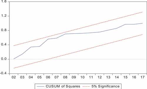
Table 5 displays the diagnostic tests of the ARDL model. Results indicate that the model does not have problems related to autocorrelation, specification error using Ramsey RESET test, the normality of residuals or heteroscedasticity. Furthermore, Figures 1 and 2 show Cumulative Sum of Recursive Residual (CUSUM) and Cumulative Sum of Squares of Recursive Residuals (CUSUMQ) tests that has no evidence of misspecification and instability during the period estimated by the model.

Figure 1. Plot of cumulative sum of recursive residuals.Source: EViews (2019)

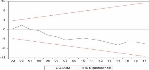
Figure 2. Plot of cumulative sum of squares of recursive residuals.Source: EViews (2019)

The Granger causality test indicated from the above result reveals that income inequality is not essential for the economic growth in Ethiopia both in the short and long run. In the long run, the ETC coefficient is positive and significant, so income inequality cannot cause economic growth, and in the short run, it is insignificant. In the long run, there is unidirectional causality running from economic growth to income inequality. In the short run, economic growth increases income inequality in Ethiopia. There is also unidirectional causality running from economic growth to income inequality both in the short run and long run.

5. Conclusion

This study examined the causal relationship between income inequality and economic growth in Ethiopia during the period from 1980 to 2017. The study employed the ARDL bound test approach to examine the long- and short-run relationship between income inequality and explanatory variables, and VECM was used to investigate the direction of causality between income inequality and economic growth. Before employing the ARDL model, the researcher has tested stationarity properties of the variables by using ADF and PP tests (Table 7). The results of the unit root test reveal that all variables are stationary after the first difference. Regarding the diagnostic and stability test, the result shows that the model is stable and desirable in the long run without any evidence of serial autocorrelation and heteroscedasticity as well as no any evidence for structural break. A bound test approach to cointegration indicated that the bound test (F-statistic) value is greater than the upper critical value, which implies that there is a long-run relationship between income inequality and its respective determinant.

Table 7. Long- and short-run causalities

	NULL HYPOTHESIS	OBS.	LAG	COEFFICIENT	PROB.
Long run	L(RGDP) does not Granger causes L(GINI)	37	1	−3.018194 (−0.435040)	0.0048***
	L(GINI) does not Granger causes L(RGDP)	37	1	2.987393 (0.047326)	0.0052
Short run	L(GINI) does not Granger causes L(RGDP)	32	3	1.976825	0.1373
	L(RGDP) does not Granger causes L(GINI)	34	2	13.37863	0.0001***

Source: EViews (2019)

The symbols *, ** and *** indicate the levels of significance at 10%, 5% and 1% to reject the null hypothesis of the direction of causality, respectively. The ETC coefficients are in brackets.

The empirical results implied the negative long-run and positive short-run impact of economic growth on income inequality in Ethiopia. The positive impact of income inequality and economic growth in Ethiopia supports the Kuznets hypothesis that the initial increase in GDP per capita leads to the increase in income inequality. This implies that income inequality act as an input to support and accelerate economic growth in the long-run and in the short-run economic growth causes income inequality. During the initial stage of development, inequality will increase with rising economic growth. The increase in inequality will reduce growth and vice versa. This pattern seems to be consistent with evidence from developing countries. With regard to control variables, except trade openness, total population and government spending on education and health, all variables significantly influence income inequality in the long run. Real GDP, gross capital formation for investment, inflation and government spending on education and health were the pioneering determinant of income inequality in the short run. Furthermore, VECM granger causality tests show that the direction of causality is running from economic growth to income inequality both in the short and long run. There are often problems with causality. For instance, there is no consensus/agreement about the direction of the relationship between income inequality and economic growth or we can say that the link between economic growth and income inequality is bi-directional, i.e. economic growth affects income inequality and vice versa. Generally, further research needs to be done to examine the relationships between income inequality and economic growth.

6. Policy implication and future directions

The study examined the causal relationship between income inequality and economic growth in Ethiopia over 37 years by applying typical Autoregressive Distributive Lag (ARDL) techniques. The finding revealed that there is a negative relationship between income inequality and economic growth in the long run. However, in the short run, there is a positive relationship. The magnitude of the ETC coefficient is −1.004961, and justified about 100.4961 percent, the disequilibrium annually converges towards long-run equilibrium. In addition, VECM granger causality tests show that unidirectional causality runs from economic growth to income inequality both in the short and long run. Based on the finding of this, the following policy implications were forwarded.

• The government should pursue and foster redistribution of income. The implementation of pro-poor growth policies that aim to boost economic growth and development while paying attention to the interests of the poor and reducing income gap is important to sustain economic growth of the country. In general, from the finding of the study, it can be concluded that the government should focus on reducing the income gap through labor force improvement and domestic resource-based capital formation to realize sound, sustainable long-run economic growth in the country.

• In fact, this work could not exhaust all specific components of the causal relationship between income inequality and economic growth in Ethiopia. Observing the impact of income inequality on economic growth and the nations of the country, future researchers need to work by considering other dimensions, which are not addressed by this study, and need to use updated data and model of analysis to come to a new result that may support or is against this research finding.

Disclosure statement

No potential conflict of interest was reported by the author(s).

Additional information

Funding

The authors received no direct funding for this research.

Notes on contributors

Mihret Wolde

Mihret Wolde (MSc in Development Economics) is a full time lecturer at Jimma University for the last five years and till now. Dr. Leta Sera (PhD in Economics) is a full time Assistant professor at the college of business and economics, Jimma University, Ethiopia. He has more than 10 years of teaching experience in total. His areas of research interest are macro issues like impact of monetary and fiscal policies analysis, on exchange rate instabilities, etc. Mr. Tesfaye Melaku (Assistant professor of Economics, MSc in Economics, and PhD Fellow at University of Antwerp) has worked for more than 8 years at the college of Business and Economics, Jimma University, Ethiopia. His research interests are program impact analysis, microfinance, poverty, Monetary and fiscal Policy Analysis and adoption of improved farm inputs. Furthermore, Mr. Tesfaye Melaku is a full member of Ethiopian Economic Association.

References

- Abebe, F. N. (2016). Determinants of income inequality in urban Ethiopia: A study of south wollo administrative zone, Amhara national and regional state. International Journal of Applied Research, 2(1), 550–16.
- Angeles-Castro. (2005). The effects of economic liberalization on income distribution: a panel data analysis. In E. Hein, A. Heise, & A. Truger (Eds.), Wages, employment, distribution and growth (pp. 151–180). Palgrave Macmillan.
- Beza, G. (2009). linkage between economic growth and income inequality in Ethiopia. International Journal of Sustainability Management and Information Technologies.
- Bigsten & Abebe. (2006). Poverty, income distribution and labour markets in Ethiopia. Nordiska Afrikainstitute.
- CSA, Central Statistical Agency of Ethiopia. (2010/2011). Agricultural sample survey.
- Eskindir (2011) The determinates of income inequality in Urban Ethiopia: The case of woldia town. https://www.researchgate.net/publication/344362397
- Fawaz, F., Rahnama, M., & Valcarcel, V. J. (2014). A refinement of the relationship between economic growth and income inequality.Applied Economics. 46, 3351–3361. CrossRef
- Gashaw Getaye. (2016). The link between economic growth and income inequality in Ethiopia.
- Gizachew, M. (2019, May). Determinant of income inequality in Ethiopia: regression based inequality decomposition. European Business & Management, 5(3), 42–50. https://doi.org/10.11648/j.ebm.20190503.12
- Granger, C. W. J., & Newbold, P. (1974). Spurious regressions in econometrics. Journal of Econometrics, 2, 111;20.
- Hamid, L. (2017). The Effects of Income inequality on economic growth evidence from MENA Countries. Eastern Illinois University.
- Hurisso, G. (2010). The propaganda of high growth and the state of economic data in Nazareth, Ethiopia.
- IMF African Dep’t. (2015). Regional economic outlook; international monetary fund. Sub-Saharan Africa Navigating Headwinds.
- Kaasa, A. (2003). Factors influencing income inequality. University of Tartu.
- Klasen, S. (2016). What to do about rising inequality in developing countries? PEGNet Policy Brief, No. 5/2016, Kiel Institute for the World Economy (IfW), Poverty Reduction, Equity and Growth Network (PEGNet).
- Kuznets, S. (1955). Economic Growth and Income Inequality. American Economic Review.
- MthuliNcube, J. C. A., & KjellHausken. (2013).Inequality Economic growth, and poverty in the middle east and north Africa.
- Narayan, P. (2005). The saving and investment nexus for china: evidence from cointegration tests. Applied Economics, 37(17), 1979–1990. https://doi.org/10.1080/00036840500278103
- Narayan, P. K., & Smyth, R. (2006). ‘The Determinants of Immigration from Fiji to New Zealand: An Empirical NARYAN & SMYTH: MIGRATION FLOWS 341 Re-Assessment Using the Bounds Testing Approach. International Migration, 41(1), 33–58.
- Nayaran, K. (2004). Reformulating critical values for the bounds F-statistics approach to cointegration: An application to the tourism demand model for Fiji. [Discussion Papers No: 02], Monash University, Victoria, Australia.
- Panizza, U. (2002). Income inequality and economic growth: Evidence from American data. Journal of Economic Growth, 7(1), 25–41. https://doi.org/10.1023/A:1013414509803
- Partridge. (2006). The Elusive Inequality-Economic Growth Relationship: Are There Differences between Cities and the Countryside? The Annals of Regional Science.
- Pesaran, M. H., Shin, Y., & Smith, R. J. (1996). Testing for the existence of a long-run relationship. DAE Working Paper, No. 9622, and Department of Applied Economics, University of Cambridge.
- Pesaran, M. H., & Shin, Y. (1999). An Autoregressive Distributed Lag Modeling Approach to Cointegration Analysis.
- Pesaran, M. H., Shin, Y., & Smith, R. J. Bounds testing approaches to the analysis of level relationship. (2001). Journal of Applied Economics, 16(3), 289–326. John Wiley & Sons, Ltd. https://doi.org/10.1002/jae.616
- Pesaran, M. H., Shin, Y., & Smith, R. (2001). Bounds testing approaches to the analysis of level relationships. Journal of Applied Econometrics, 16, 289–326.
- Sisay, D., & Efta, H. (2020). Analysis of poverty, income inequality and their effects on food insecurity in southern Ethiopia.
- Tadesse, W. (2019). The determinates of income inequality in Urban Ethiopia: The case of Woldia Town. https://www.researchgate.net/publication/344362397
- Tassew, W., Hoddinott, J., & Dercon, S. (2009). Poverty and Inequality in Ethiopia: 1995/96-2004/05. Addis Ababa University, International Food Policy Research Institute and University of Oxford, Addis Ababa.
- Tigist, G., & Maru, S. (2018). Relationship between Income Inequality and Economic Growth in Ethiopia.
- Wahiba, N. F., & Weriemmi, M. E. (2014). The Relationship between Economic Growth and Income Inequality. International Journal of Economics and Financial Issues, 4(1).
- World Bank. (2015). 2014 Ethiopia Poverty Assessment.
- World Bank. (2017). Ethiopia GDP per capita PPP. Retrieved September 2, 2017) from https://tradingeconomics.com/ethiopia/gdp-per-capita-ppp