The asymmetric and non-linear relationship between capital flight and economic growth nexus

Abstract

The paper sought to explore the effect of capital flight on the economic growth nexus in Ghana. The study used quarterly time series data from 1976 to 2020 to test three hypotheses. The paper used non-linear autoregressive distributive lagged employing unit root test, co-integration test, and Wald test to assess the asymmetrical relationship among the variables. The study posits that both the positive and negative changes in capital flight affect economic growth significantly. Again, the study revealed that capital flight and other macroeconomic variables explain about 75.28% of economic growth. Furthermore, the model can restore the short-run relationship to the dynamic long-long equilibrium at the speed of 35.6%. The study recommends that government economic policymakers build economic confidence by stabilizing economic conditions in the country to reduce the incentives for capital outflows. Further, as a priority, the government must formulate strategies to recover looted public funds by corrupt public officials stacked in foreign accounts and inject them into the economy to boost economic growth.

Keywords:

• asymmetric
• relationship
• capital flight
• panel
• model
• economic growth
• NARDL

1. Introduction

Capital flight is characterized by large outflows of assets from a country due to several events resulting in negative economic consequences. The issue of capital flight has become a severe issue in many developing countries because of its effects on economic growth, macroeconomic stability, and people’s income distribution and welfare (Zheng & Tang, 2009). Walter (1987) defines capital flight as all capital that “flees” regardless of the motive. Part of domestic savings sent abroad due to adverse economic consequences would eventually adversely affect that country’s economic fortunes. Capital flight’s long-term adverse (negative) effect includes worsening capital scarcity and further capital formation. Capital flight can be legal or illegal. Capital flight occurs in several ways: bank transfers using cash or monetary instruments; where investors and businesses remove money and assets from a country; movement of precious metals and collectibles where local currency is swapped for other precious metals; transfer through false invoicing of trade transactions; black market transfers of funds abroad, transfers overseas through commissions and agent fees locally earned among others. The legal movement of capital flight is in search of investment opportunities outside the country and is documented for accounting. This illicit capital outflow is an illicit financial outflow that escapes the country’s economic, institutional and political risk and avoids accounting purposes. Capital flight has affected some countries negatively, while others have gained substantially from the illicit capital outflows.

The current decade has seen intense discussions on capital flight from both literature and the development policy discourse; due to the adverse economic consequence, especially for those in Africa and Sub-Saharan Africa. It is estimated that African countries lost up to 1.3 trillion dollars (in 2010, constant U.S. dollars) to capital flight between 1970 and 2010 (Ajayi & n.d.ikumana, 2015; Boyce & Ndikumana, 2012). Assuming that this capital outflow earned the modest interest rate measured by the short-term United States Treasury Bill rate, this would earn substantial returns for those countries within Africa and Sub-Saharan Africa. This dilemma has intensified in sub-Saharan countries after the debt crises that span from the late 1980s to the early 1990s, adversely affecting several African economies (Osei-Assibey et al., 2018). Specifically, 33 Sub-Saharan economies lost 814 billion dollars between 1970 and 2012 (Boyce, 2012) due to illicit capital flight. The hostile macroeconomic and political environment in most developing economies accounts for the substantial capital flight from these economies. These include corruption, terrorism, governance, regulation quality, exchange duality, public sector indebtedness, political instability, domestic investment, and private sector credit (Vu & Zak, 2006).

Several studies on the relationship between capital flight and economic growth yielded mixed outcomes. Some researchers concluded that there was a negative relationship between capital flight and economic development (Bredino et al., 2018; Cervena, 2006; Henry, 2013; Lawal et al., 2017; Orji et al., 2020), while other researchers concluded there was a positive relationship with economic growth (A. S. n.d.iaye, 2014; Oluwaseyi1, 2017; Davies, 2008; Akanbi, 2015; Ajilore, 2015; Lawanson, 2007). From the perspective of Endogenous growth theory, government policies that increase capital formation (i.e., ensure investment in physical capital) and knowledge (i.e., technology) should lead to an increase in economic growth (Romer, 1986; Lucas, 1988). The situation explains why capital flight negatively affects a country’s economic resources leading to retard economic growth. Researchers’ mixed relationship reported between capital flight, and economic growth requires an in-depth examination to help direct the future short-run and long-run policy formation. Again, most previous studies examined the capital flight and economic growth relationship with a focus on the short-run effect and excluded the long-run effect (Bakare, 2011; Forson et al., 2017; Ndikumana, 2016; Tjaondjo, 2019). Furthermore, these studies employed less robust methodologies involving ordinary least square (OLS) and Linear Autoregressive Distributed lag (ARDL) to assess the relationship between capital flight and economic growth and concluded that capital flight significantly decreases economic growth. However, the recent studies by Anderl and Caporale (2021) and Cho et al. (2021) using the Non-linear autoregressive distributed lag (NARDL) model have outperformed those that used ARDL to examine the economic growth capital flight nexus.

Furthermore, in recent times, especially from 2007 onwards, the Ghanaian economy has experienced an increasing rate of capital flight and, at the same time, recorded an appreciable growth rate (The World Bank, World Development Indicators, 2021). This relationship between increasing capital flight and economic growth in the Ghanaian economy is at variance with economic literature. Based on these premises, the current study seeks to examine the role of capital flight on the economic growth in Ghana. The primary motivation for this paper is to evaluate the monetary policy’s position on the effect of the capital flight nexus in Ghana. We submit that this study is essential for the following reasons: Firstly, the study aimed to employ an alternative, recent, and more robust methodology like NARDL to assess the effect of capital flight on economic growth, purposely to avoid some of the shortcomings of the OLS and ARDL used in the past. Secondly, the results will provide fresh insight and clarity to some of the relationships between a country’s macroeconomic fundamentals, such as interest rate and inflation rate, to assist government monetary policy direction. Finally, the result supports the literature and helps policymakers understand the relationship between capital flight and economic growth to ensure the economy performs efficiently. Section 2 reviews existing literature, followed by the research methodology in section 3. Section 4 presents the results and the attendant discussion of the research results. Finally, the study ends with some conclusions and limitations for the study.

2. Literature review

This section reviewed related literature on capital flight and economic growth. The section is organized into two sections: Theoretical review and empirical review.

2.1. Theoretical review: endogenous growth theory

Endogenous growth theory was introduced by Robert Lucas of The University of Chicago. The main promulgators of the theory were Lucas (1988) and Romer (1994), and were espoused due to some criticisms against the Neoclassical (Exogenous growth) theory on economic growth. Endogenous growth theory is referred to as the New Growth Theory. The approach is based on the aggregate production function, which specifies how specific inputs on physical capital, human capital, and technology can lead to the output. The advantage of the aggregate production function is that it enables economic growth to be represented mathematically, and it is expressed as equation (1)(1) $Y_t=A_{t}f(K_t^{\beta },L_t^{\alpha })$(1) :

(1) $Y_t=A_{t}f(K_t^{\beta },L_t^{\alpha })$(1)

The aggregate production function is exceptionally good at summarizing aggregate production in the economy. Where Y denotes the aggregate production function (i.e., GDP growth rate per annum) at the time t, A is the adjustment factor outside the production function. It is used to capture the effect of changes in technology at the time t, K represents physical capital stock at the time t, and L represents human capital at the time t. The superscripts represented by α and β are the output elasticity of physical capital stock and human capital, respectively. There are two main assumptions or forces driving the theory: Firstly, a policy aimed to increase capital formation (i.e., to ensure investment in physical capital) and technology (i.e., knowledge) should lead to an increase in economic growth (Romer, 1986; Lucas, 1988). When technological development meets with capital for investment, then economic growth is optimized. This makes capital and technology the right combination of the sources of growth that plays a central role in the growth of any economy. Secondly, the output’s elasticity of physical capital stock and human capital are assumed to be constant and influenced by technologies. Capital can be used to acquire the superior technology or invested in human capital to acquire new knowledge and skills to propel economic growth. It explains why technology is considered an adjustment factor outside production function. Therefore, a country with sufficient capital can invest in research and knowledge acquisition to lead to economic growth.

In contrast, a country without adequate capital cannot acquire the latest technology with the attendant unskilled labour leading to retarded growth and a vicious cycle of poverty in the economic development. A country like Taiwan broke from a vicious cycle of poverty to a growth path due to consistent economic policies to attract foreign capital for investment. The considerable economic growth and development in Taiwan is attributed especially to the enactment of new investment law in the 1960ʹs to encourage direct investment by foreign and overseas Chinese capital for investments (Irwin, 2021; Jao, 1976). Capital flight is mainly in the form of physical capital and human capital. It is based on the assumption that optimal capital can be the requisite investment technology for growth. It implies that capital inflow can cause economic growth while capital outflow from a country can cause economic retardation. Most developing countries experienced a capital flight to advanced countries due to economic and political uncertainties (Lawal et al., 2017; A. S. n.d.iaye, 2014). The economic and political forces create uncertainty that causes capital flight from domestic regions relative to better investment opportunities in advanced nations. These better alternatives result in the movement of investible resources transferred to developed economies with high-interest rates and large varieties of financial instruments as a result of economic growth as well as political stability. This creates a shortage of capital in developing economies, causing a savings gap, constraining aggregate investment, and limping economic growth (Onodugo et al., 2014).

Consistent with endogenous growth theory, the capital flight in developing countries has created adverse macroeconomic effects on developing countries leading to a decline in aggregate investment, low economic growth, declining employment, increased dependency ratio, and a high death rate. Again, the endogenous growth theory provides significant literature explaining why some countries are lesser developed countries (LDC) and others are considered developed countries. The view is built on the idea that an increase in capital accumulation (i.e., capital inflow) or deterioration in capital accumulation (i.e., capital outflow or capital flight) can positively or negatively affect economic growth. Therefore, the adverse effect of capital flight resulting from economic and political uncertainties explains the economic deprivation in most of the LDC (Boyce & Ndikumana, 2012; Eshete, 2018; Osei-Assibey et al., 2018).

3. Methodology

This study is empirical research involving a quantitative research method to collect secondary data to measure phenomena and test research hypotheses (Moyo & Munoriyarwa, 2021). The study uses Quarterly time series data from 1976 to 2020 gleaned from the World Development Indicators (WDI) of the World Bank, the Bank of Ghana (BoG) database, and Political Economy and Research Institute (PERI) to assess the relationship among the variables. The study applied these econometrics tools: Unit root test, bounds test, Non-linear Auto Regressive Distributed Lag (NARDL) model, diagnostic tests, and estimations of the short-run and long-run impacts are applied to the data collected. Eview 10.0 is the analytical software used in carrying out the analysis.

3.1. Research variables

The data collected are organized into dependent, independent, and control variables to assess the effect of the capital flight on the economic growth nexus.

3.1.1. Dependent variable (i.e., GDP growth rate)

Gross Domestic Products (GDP) growth rate: GDP is the proxy used to measure the dependent variable for this study. The GDP growth rate is GDP’s annual percentage growth rate at market prices based on constant local currency. Data is taken from the World Development Indicator (WDI) and Bank of Ghana (BoG). The subsequent studies used GDP as the proxy for economic growth (King & Levine, 1993; Nguena & Abimbola, 2003).

3.1.2. Independent variables (i.e., capital flight)

Capital Flight (CF): This is an independent variable. The proxy measures the external debt of foreign direct investment minus current accounts plus foreign reserves. Data is taken World Development Indicator (WDI). There were mixed outcomes on the relationship between capital flight and economic growth. The following researchers concluded there was a negative relationship between capital flight and economic development (Bredino et al., 2018; Cervena, 2006; Henry, 2013; Lawal et al., 2017; Orji et al., 2020), while the following researchers concluded there was a positive relationship with economic growth (A. S. n.d.iaye, 2014; Oluwaseyi1, 2017; Davies, 2008; Akanbi, 2015; Ajilore, 2010; Lawanson, 2007).

3.1.3. Control variables (i.e., inflation and interest rates)

Besides the well-established fact that capital flight can influence economic growth, other external factors can also affect economic growth. These external factors are known as control variables. The study used inflation and interest rates as control variables for this study.

Inflation (INF): This is an independent variable. Inflation reflects the potential risk of over-heating caused by increased credit granted to the private sector. Empirical studies show that inflation affects economic growth negatively (Boyd et al., 2001; Borio, English & Filardo, 2003 en World Development Indicator (WDI).

Interest rates (INT): The interest rate is the cost of borrowing money in an economy, and it is the primary determinant of the cost of credits in an economy. The proxy is InINT, and its equivalent percentage (%) measures the 91-Day Treasury bill Interest rate. Previous studies documented a mixed relationship between interest rate and economic growth. The following researchers opined a negative relationship between interest rates and economic development (Harswari & Hamza, 2017; Hye & Wizarat, 2013). The researchers opined a positive relationship between interest rates and economic growth (Khalid & Nasir, 2004; Mushtaq & Siddiqui, 2016; Orji et al., 2015; Salahuddin & Gow, 2009).

3.2. Model specification

The regression model for this study is based on the recent contribution of Léonce that stems from the theoretical framework of the Endogenous growth theory of aggregate production function. The model was modified to include inflation (INF) and interest rate (INT) and expressed as equation (2)(2) $GD{P}_t={\beta }_0+{\beta }_{1}C{F}_t+{\beta }_{2}IN{F}_t+{\beta }_{3}IN{T}_t+{\mu }_t$(2) :

(2) $GD{P}_t={\beta }_0+{\beta }_{1}C{F}_t+{\beta }_{2}IN{F}_t+{\beta }_{3}IN{T}_t+{\mu }_t$(2)

Where:

GDP represents GDP growth domestic products, CF represents capital flight, INF represents inflation, and INT represents interest rate. We cannot proceed with the functional equation, so log-linear was taken to transform the applicable equation in (1(1) $Y_t=A_{t}f(K_t^{\beta },L_t^{\alpha })$(1) ) into equation (3)(3) $InGD{P}_t={\beta }_0+{\beta }_{1}InC{F}_t+{\beta }_{2}InIN{F}_t+{\beta }_{3}InIN{T}_t+{\mu }_t$(3) as follows:

(3) $InGD{P}_t={\beta }_0+{\beta }_{1}InC{F}_t+{\beta }_{2}InIN{F}_t+{\beta }_{3}InIN{T}_t+{\mu }_t$(3)

Equation (2)(2) $GD{P}_t={\beta }_0+{\beta }_{1}C{F}_t+{\beta }_{2}IN{F}_t+{\beta }_{3}IN{T}_t+{\mu }_t$(2) is an ordinary least square (O.L.S.) regression approach. It can assess the linear relationship between the CF, INT, INF, and G.D.P but cannot simultaneously evaluate the short-run and long-run relationship between the variables. Subsequently, equation (3)(3) $InGD{P}_t={\beta }_0+{\beta }_{1}InC{F}_t+{\beta }_{2}InIN{F}_t+{\beta }_{3}InIN{T}_t+{\mu }_t$(3) is written in a linear auto-regression distribution lag (linear ARDL.) form as equation (4)(4) $\begin{array}{rl}& \mathrm{\Delta }InGD{P}_t={\beta }_0+{\beta }_{1}InGD{P}_{t-1}+{\beta }_{2}InC{F}_{t-1}+{\beta }_{3}InIN{T}_{t-1}+{\beta }_{4}InIN{F}_{t-1}+\sum _{i=1}^m{\lambda }_i\mathrm{\Delta }InGD{P}_{t-1}+\sum _{i=0}^n{\lambda }_i\mathrm{\Delta }InC{F}_{t-1}\\ & \sum _{i=0}^p{\lambda }_i\mathrm{\Delta }InIN{T}_{t-1}+\sum _{i=0}^q{\lambda }_i\mathrm{\Delta }InInIN{F}_{t-1}+\psi EC{T}_{t-1}+{\mu }_t\end{array}$(4) . This is an appropriate approach for generating short-run and long-run statistics between variables (Duasa, 2007). The linear ARDL model to consider all the dynamic changes of the dependent variable from the changes in the lagged values of the independent variables required a linear autoregressive distributed lagged (ARDL.) model by Pesaran et al. (2001). In the past, the most assessment was centered on the effect of capital flight on economic growth using linear relationships. This is usually centered in one direction of capital flight based on net capital flights (i.e., capital inflows less capital outflows) and has caused a lot of inconsistencies in outcomes in the past. Unfortunately, the linear ARDL cannot interpret and estimate asymmetric coefficients but can be used to test for co-integration and expressed as equation (4)(4) $\begin{array}{rl}& \mathrm{\Delta }InGD{P}_t={\beta }_0+{\beta }_{1}InGD{P}_{t-1}+{\beta }_{2}InC{F}_{t-1}+{\beta }_{3}InIN{T}_{t-1}+{\beta }_{4}InIN{F}_{t-1}+\sum _{i=1}^m{\lambda }_i\mathrm{\Delta }InGD{P}_{t-1}+\sum _{i=0}^n{\lambda }_i\mathrm{\Delta }InC{F}_{t-1}\\ & \sum _{i=0}^p{\lambda }_i\mathrm{\Delta }InIN{T}_{t-1}+\sum _{i=0}^q{\lambda }_i\mathrm{\Delta }InInIN{F}_{t-1}+\psi EC{T}_{t-1}+{\mu }_t\end{array}$(4) :

(4) $\begin{array}{rl}& \mathrm{\Delta }InGD{P}_t={\beta }_0+{\beta }_{1}InGD{P}_{t-1}+{\beta }_{2}InC{F}_{t-1}+{\beta }_{3}InIN{T}_{t-1}+{\beta }_{4}InIN{F}_{t-1}+\sum _{i=1}^m{\lambda }_i\mathrm{\Delta }InGD{P}_{t-1}+\sum _{i=0}^n{\lambda }_i\mathrm{\Delta }InC{F}_{t-1}\\ & \sum _{i=0}^p{\lambda }_i\mathrm{\Delta }InIN{T}_{t-1}+\sum _{i=0}^q{\lambda }_i\mathrm{\Delta }InInIN{F}_{t-1}+\psi EC{T}_{t-1}+{\mu }_t\end{array}$(4)

The study will use the NARDL approach instead of linear ARDL to decompose the independent variables (i.e., CF, INT, and INF). The new approach introduced by Shin et al. (2014) can overcome the inconsistencies in outcome from linear ARDL and can assist in assessing the impact of the short-run, long-run, and the asymmetrical relationship between negative and positive changes in capital flight on ex = conomic growth in Ghana,

Where:

$C{F}_t^{+}$ $C{F}_t^{-}$ are the partial sums of the positive changes and the negative changes in the CF series, $IN{T}_t^{+}$ and $IN{T}_t^{-}$ are the partial sums of the positive changes and the negative changes in the INT, $IN{F}_t^{+}$ and $IN{F}_t^{-}$ are the partial sums of the positive changes and the negative changes in the INF series. These are expressed as equations (5)(5) $C{F}_t^{+}=\sum _{i=1}^t\mathrm{\Delta }C{F}_t^{+}=\sum _{i=1}^{t}max(\mathrm{\Delta }C{F}_i,0)$(5) , (6(6) $C{F}_t^{-}=\sum _{i=1}^t\mathrm{\Delta }C{F}_t^{-}=\sum _{i=1}^{t}max(\mathrm{\Delta }C{F}_i,0)$(6) ), (7(7) $IN{T}_t^{+}=\sum _{i=1}^t\mathrm{\Delta }IN{T}_t^{+}=\sum _{i=1}^{t}max(\mathrm{\Delta }IN{T}_i,0)$(7) ), (8(8) $IN{T}_t^{-}=\sum _{i=1}^t\mathrm{\Delta }IN{T}_t^{-}=\sum _{i=1}^{t}max(\mathrm{\Delta }IN{T}_i,0)$(8) ), and (9(9) $IN{F}_t^{+}=\sum _{i=1}^t\mathrm{\Delta }IN{F}_t^{+}=\sum _{i=1}^{t}max(\mathrm{\Delta }IN{F}_i,0)$(9) ) in this study:

(5) $C{F}_t^{+}=\sum _{i=1}^t\mathrm{\Delta }C{F}_t^{+}=\sum _{i=1}^{t}max(\mathrm{\Delta }C{F}_i,0)$(5)

(6) $C{F}_t^{-}=\sum _{i=1}^t\mathrm{\Delta }C{F}_t^{-}=\sum _{i=1}^{t}max(\mathrm{\Delta }C{F}_i,0)$(6)

(7) $IN{T}_t^{+}=\sum _{i=1}^t\mathrm{\Delta }IN{T}_t^{+}=\sum _{i=1}^{t}max(\mathrm{\Delta }IN{T}_i,0)$(7)

(8) $IN{T}_t^{-}=\sum _{i=1}^t\mathrm{\Delta }IN{T}_t^{-}=\sum _{i=1}^{t}max(\mathrm{\Delta }IN{T}_i,0)$(8)

(9) $IN{F}_t^{+}=\sum _{i=1}^t\mathrm{\Delta }IN{F}_t^{+}=\sum _{i=1}^{t}max(\mathrm{\Delta }IN{F}_i,0)$(9)

(10) $IN{F}_t^{-}=\sum _{i=1}^t\mathrm{\Delta }IN{F}_t^{-}=\sum _{i=1}^{t}max(\mathrm{\Delta }IN{F}_i,0)$(10)

The study used the NARDL model to formulate three different cases such as (1) long-run and short-run asymmetry of capital flight on economic growth, (2) long-run asymmetry of capital flight on economic growth only, and (3) short-run asymmetry of capital flight on economic growth only. The advantages of using the NARDL model instead of the ARDL model are that the NARDL model can isolate and estimate the effect of different directional changes of capital flight (i.e., outflow and inflows) on economic growth. Secondly, the NARDL approach is an improvement to the linear ARDL Equation (3)(3) $InGD{P}_t={\beta }_0+{\beta }_{1}InC{F}_t+{\beta }_{2}InIN{F}_t+{\beta }_{3}InIN{T}_t+{\mu }_t$(3) decomposed capital flight into the positive and negative changes under the NARDL model, the partial sum of positive and negative variables values are generated and presented as equation (5)(5) $C{F}_t^{+}=\sum _{i=1}^t\mathrm{\Delta }C{F}_t^{+}=\sum _{i=1}^{t}max(\mathrm{\Delta }C{F}_i,0)$(5) to (10(10) $IN{F}_t^{-}=\sum _{i=1}^t\mathrm{\Delta }IN{F}_t^{-}=\sum _{i=1}^{t}max(\mathrm{\Delta }IN{F}_i,0)$(10) ) are incorporated to arrive at equation (11)(11) $\begin{array}{rl}& \mathrm{\Delta }InGD{P}_t={\beta }_0+{\beta }_{1}InGD{P}_{t-1}+{\beta }_{2}InC{F}_{t-1}^{+}+{\beta }_{3}InC{F}_{t-1}^{-}+{\beta }_{4}InIN{T}_{t-1}^{-}+{\beta }_{5}InIN{T}_{t-1}^{-}+{\beta }_{6}InIN{F}_{t-1}^{-}\\ & +{\beta }_{7}InIN{F}_{t-1}^{-}+\sum _{i=1}^m{\lambda }_i\mathrm{\Delta }InGD{P}_{t-i}+\sum _{i=0}^n({\lambda }_i\mathrm{\Delta }InC{F}_{t-i}^{+}+{\lambda }_i\mathrm{\Delta }InC{F}_{t-i}^{+})+\sum _{i=0}^p({\lambda }_i\mathrm{\Delta }InIN{T}_{t-i}^{-}+{\lambda }_i\mathrm{\Delta }InIN{T}_{t-i}^{-})\\ & +\sum _{i=0}^q({\lambda }_i\mathrm{\Delta }InIN{F}_{t-i}^{-}+{\lambda }_i\mathrm{\Delta }InIN{F}_{t-i}^{-})+\psi EC{T}_{t-1}+{\mu }_t\end{array}$(11) . Again, NARDL is more robust and permits the estimation of both dynamics of the negative and positive changes in independent variables on a specific dependent variable (Adekunle & n.d.ukwe, 2018). Lastly, the NARDL allows the variables to have different optimal lags and employs a single reduced form equation to determine long- and short-run relationships among variables (Pesaran et al., 2001). On the other hand, it measures the short-run and long-run impacts of the C.F., INT, and INF on the G.D.P.

(11) $\begin{array}{rl}& \mathrm{\Delta }InGD{P}_t={\beta }_0+{\beta }_{1}InGD{P}_{t-1}+{\beta }_{2}InC{F}_{t-1}^{+}+{\beta }_{3}InC{F}_{t-1}^{-}+{\beta }_{4}InIN{T}_{t-1}^{-}+{\beta }_{5}InIN{T}_{t-1}^{-}+{\beta }_{6}InIN{F}_{t-1}^{-}\\ & +{\beta }_{7}InIN{F}_{t-1}^{-}+\sum _{i=1}^m{\lambda }_i\mathrm{\Delta }InGD{P}_{t-i}+\sum _{i=0}^n({\lambda }_i\mathrm{\Delta }InC{F}_{t-i}^{+}+{\lambda }_i\mathrm{\Delta }InC{F}_{t-i}^{+})+\sum _{i=0}^p({\lambda }_i\mathrm{\Delta }InIN{T}_{t-i}^{-}+{\lambda }_i\mathrm{\Delta }InIN{T}_{t-i}^{-})\\ & +\sum _{i=0}^q({\lambda }_i\mathrm{\Delta }InIN{F}_{t-i}^{-}+{\lambda }_i\mathrm{\Delta }InIN{F}_{t-i}^{-})+\psi EC{T}_{t-1}+{\mu }_t\end{array}$(11)

Where Δ is the difference operator, m, n, p, and q represent the lag orders. Moreover, α + = −β2/β1, α − = −β3/β1, are the coefficients of long-run effects of CF, INT, and INF increases and decreases respectively for GDP. $\sum _{i=0}^n({\lambda }_i^{+}+{\lambda }_i^{-})$ The µ is the error term or the equation’s constant, the t represents the period from 1975 to 2020, ψ represents the speed of adjustment, and $EC{T}_{t-1}$ the lagged error correction term is derived from the model. The sign, size, and statistical significance of the coefficient $EC{T}_{t-1}$ must be negative and significant to ensure convergence of the dynamics to the long-run equilibrium (Adefeso, Egbetunde & Alley, 2013). When the error correction model is negative and significant implies that the past equilibrium plays a role in determining the current outcomes of the model. The value of the coefficient, ψ, ranges typically from—1 and 0. A—1 signifies perfect and instantaneous convergence, while 0 means no adjustment after a shock in the process.

3.3. Research hypotheses development

The following hypotheses were espoused to assess the asymmetrical relationship between capital flight and economic growth so that inference can be made for this study:

H01: There is no asymmetrical relationship between capital flight (CF) and economic growth (GDP) in the short and long run. Hence, Capital flight can be decomposed into their partial sum of positive and negative changes for the study.

H02: There is no significant relationship between the positive change of the partial sum of capital flight (CF_POS) and economic growth (GDP). Hence, the positive change in capital flight cannot affect economic growth in the long run.

H03: There is no significant relationship between the negative change of the partial sum of capital flight (CF_NEG) and economic growth (GDP). Hence, the negative change of the partial sum of capital flight cannot affect the economic growth in the long run.

The study will use the NARDL approach as a statistical analysis tool to assess these hypotheses. Each hypothesis may be accepted or rejected based on the outcome of the t-statistic combined with the p-value, at a 5% significance level as the decision criteria.

4. Results and discussion

This sub-section presents the empirical findings obtained from the descriptive statistics, Pearson correlation, and non-linear autoregressive distributed lag model to test and quantify the causal relationship between capital flight and economic growth.

4.1. Descriptive statistics

Descriptive statistics provide the foundation for comparing the variables before inferential statistics. Descriptive statistics describe the entire data as a single measurement is based on the primary measures of the descriptive statistics: mean, standard deviation, minimum and maximum. The means help identify any possible irregularities before inferential statistics, while the standard deviation discloses the dispersion from the mean or the observation.

Table 1 shows that the mean for GDP, CF, INT, and INF are 8.899, 22.035, 2.946, and 3.194, respectively. The standard deviation for GDP, CF, INT, and INF are 0.304, 0.855, 0.470, and 0.698, respectively. The standard deviation is used to measure the spread, and it reveals how close each observed value is to the mean of the dataset.

Table 1. Descriptive statistics

Variables	Mean	Std. Dev.	Max	Min	Skew	Kurtosis	Jarque-Bera	Probability
GDP	8.899	0.304	9.369	6.943	0.101	2.094	4.792	0.091
CF	22.035	0.855	23.507	20.001	0.087	2.197	5.263	0.072
INT	2.946	0.47	3.756	1.805	0.306	2.189	5.597	0.061
INF	3.194	0.698	4.811	1.964	0.045	2.287	5.677	0.059

The standard deviation for GDP, CF, INT, and INF are 0.101, 0.087, 0.306 and 0.0.045. This implies the standard is low and clusters around the mean. A low standard deviation shows reliable data for the estimation. Additionally, Table 1 provides information on skewness and kurtosis. The measures of skewness and kurtosis are used to determine if the dataset met the assumption of normality (Kline, 2011). The acceptable skewness values should be between −2 and +2, and that kurtosis should be between −7 and +7 when assessing normality in regression (Byrne, 2010; George & Mallery, 2010). The result shows that GDP, CF, INT, and INF exhibit a positive skewness and are closer to zero. A positive skewness implies that the dataset is positively skewed and that the right tail is longer than the left. Therefore, the skewness for GDP, CF, INT, and INF are approximately symmetrical. The kurtosis for GDP, CF, INF, and INT are 2.094, 2.197, 2.189, and 2.287, respectively. The kurtoses values of the variables are closer to 3, implying the distribution is normal. A kurtosis of value lowers than three corresponds to a broadening of the peak and “thickening” of the tails. Therefore, it is platycurtic as it mirrors a normal distribution. Therefore, the null hypothesis of the Jarque–Bera test shows that the distribution is normal since the p-values are significant (i.e., p-value greater than 5%).

4.2. Pearson correlation matrix

This sub-section used Pearson correlation to assess the association between the variables. Using the correlation matrix ensures a relationship between dependent, independent variables and confirms an absence of multicollinearity problems among the independent variables. Pearson correlation uses the coefficient index (r) to determine the strength of the relationship between the dependent and independent variables, with r ranging from −1 to +1. The results of the correlation between the capital flight (CF), interest rate (INT) and inflation (INF), and economic growth (GDP) are presented in Table 2. Table 2 shows that the correlation index (r) between GDP and CF, INT, and INF are 0.669, 0.586, and (0.502), respectively. The result shows a significant and robust relationship among the variables, and none of the independent variables has violated the multicollinearity assumption. The result shows a positive correlation between CF, INT, and GDP, while INF and GDP are negative. A positive relationship between capital flight and economic growth means that when capital flight increases, economic growth increases vice versa. In contrast, the negative relationship between inflation and economic growth means that an increase in inflation reduces economic growth negatively (i.e., 0.70) and vice versa.

Table 2. Correlation matrix

Variables	GDP	CF	INT	INF
GDP	1.000
	—–
CF	0.669	1.000
	0.000	—–
INT	0.586	0.390	1.000
	0.000	0.000	—–
INF	(0.502)	(0.311)	(0.291)	1.000
	0.000	0.000	0.000	—–

Source: Author’s computation (2021)

According to Gujarati (2003), multicollinearity is a severe problem if the Pearson correlation coefficient between two explanatory variables is more than 0.95. Multicollinearity problems arise when there is a correlation between the independent variables. A multicollinearity problem may cause a wrong interpretation of the coefficients of the variables. Therefore, once detected, it is essential to eliminate those variables.

4.3. Results of non-linear autoregressive distributed lagged

The results from the NARDL model are organized and summarised into four significant steps: (1) establishing the time series is stationary, (2) establishing whether there is a long-run co-integration among the variables in equation (4)(4) $\begin{array}{rl}& \mathrm{\Delta }InGD{P}_t={\beta }_0+{\beta }_{1}InGD{P}_{t-1}+{\beta }_{2}InC{F}_{t-1}+{\beta }_{3}InIN{T}_{t-1}+{\beta }_{4}InIN{F}_{t-1}+\sum _{i=1}^m{\lambda }_i\mathrm{\Delta }InGD{P}_{t-1}+\sum _{i=0}^n{\lambda }_i\mathrm{\Delta }InC{F}_{t-1}\\ & \sum _{i=0}^p{\lambda }_i\mathrm{\Delta }InIN{T}_{t-1}+\sum _{i=0}^q{\lambda }_i\mathrm{\Delta }InInIN{F}_{t-1}+\psi EC{T}_{t-1}+{\mu }_t\end{array}$(4) . The NARDL model allows the study to conclude a linear long-run relationship between capital flight and economic growth and estimate the long- and short-run coefficients. (3) The study will use the NARDL model to estimate the two variables (i.e., the negative and positive) of the non-linear co-integration. Finally, there is the existence of co-integration, then the study will estimate the asymmetric responses of capital flight to economic and test the presence of short and long-run asymmetries based on the Wald test

4.3.1. Unit root test results

In statistical analysis, Augmented Dickey–Fuller (ADF) test, Philip-Perron (PP) test, and KPSS test are used to test for the existence of stationarity in time series. This study used the ADF test to test for stationarity or unit roots in the data and not the PP test and KPSS test because the results of the ADF test are similar to the PP test and KPSS test but under slightly different conditions. According to Arltova (2016), ADF testing is more reliable. It gives a perfect result, especially in the case with many observations, while the PP test and KPSS are substitutes for concise time series. Therefore, the study settled on the ADF test because the observation span from 1976 to 2020 is large enough to consider the ADF test as the preferred test. According to Granger and Newbold (1974), the data for the research should be non-stationary (i.e., unit root) to prevent spurious regression outcomes for the study. The ADF test results are presented in Table 3:

Table 3. Results of stationarity test (augmented dickey–fuller test)

	Level		1st difference
	ADF T-statistics	1% Critical Value	ADF T-statistics	1% Critical Value	Order of int
GDP	−1.930	−3.032	−5.020***	−4.905216***	I(1)
CF	−2.186	−1.945	−4.885***	−4.862682***	I(1)
INF	−1.548	−3.588	−4.873***	−4.855297***	I(1)
INT	−2.892	−1.955	−4.160***	−4.383056***	I(1)

***, **, and * denote rejection of the null hypothesis at the 1%, 5%, and 10% significance levels, respectively.

Source: Researcher’s computation (Eviews 10.0)

The empirical result from Table 3 indicates some of the variables (i.e., CF and INT) stationary at the level I(0) but GDP and INF were not stationary at level. However, all variables become stationary at the first difference I(1). When the variables exhibit mixed integration of I(0) and I(1), then autoregressive distributive lag (ARDL) is the most suitable for the regression (Shrestha & Bhatta, 2018). Secondly, none of the variables was integrated at order two, i.e., I (2) in the ARDL model. Therefore, the series are integrated at the same order of co-integration. It is observed that ADF test statistics are more significant than the 1% and 5% critical values.

4.3.2. Results of bounds test for co-integration

Therefore, the study established the existence of long-run co-integration among the variables. The F-test value is used to compare the lower and upper bounds. According to Pesaran et al. (2001) and later modified by Shin et al. (2014), the decision criteria is that once the calculated F-value is higher than the upper bound, the null hypothesis is rejected in favor of the alternate theory:

$H_0:\rho ={\phi }_1^{+}={\phi }_2^{-}={\phi }_3^{+}={\phi }_4^{-}={\phi }_5^{+}={\phi }_6^{-}=0$

$H_1:\rho \ne {\phi }_1^{+}\ne {\phi }_2^{-}\ne {\phi }_3^{+}\ne {\phi }_4^{-}\ne {\phi }_5^{+}\ne {\phi }_6^{-}\ne 0$

Table 4 shows that F-statistics is 42.389 and exceeds the critical values for I(0) and I(1), respectively. The result from the ARDL bounds test indicates that there is a co-integration (i.e., long-run relationship) between capital flight and economic growth since the value of the critical F-statistics is higher than the lower bounds I(0) and upper bounds I(1) values. Therefore, the null hypothesis of no co-integration among the variables is rejected at 1%, 2.5%, 5%, and 10% significance levels, respectively.

Table 4. ARDL bounds test for the cointegrating relationship

K	Test statistics	Significance	Lower value, I(0)	Upper value, I(1)
4	F-statistics = 42.389	10%	2.53	3.59
		5%	2.87	4.00
		2.5%	3.19	4.38
		1%	3.6	4.9

Source: Researchers’ computation (2021)

4.3.3. Results from asymmetry test (i.e., wald test)

The Wald test of asymmetry for both long-run and short-run is presented in Table 5. The Wald test is used to check for the null hypothesis of no asymmetry for the long run and short run in the NARDL model. The Wald test is used to determine if the independent variables in the model are significant. The Wald test assessment is done in addition to the F-statistics to confirm co-integration among the variables in Table 4.

Table 5. Wald test statistics for long run and short-run asymmetry

	Long Run Asymmetry		Short Run Asymmetry
Variables	Chi-square	Prob.	Chi-square	Prob.
Capital flight	22.57543	0.0000	4.362191	0.0367
Inflation	54.48652	0.0000	40.10878	0.0000
Interest	13.45349	0.0002	2.193184	0.1386

Source: Researchers’ computation (2021)

Therefore, the null hypothesis (H01) that there is no asymmetry for the short and long run for the positive and negative changes for all the independent variables is rejected based on the information shown in Table 5. It concludes that capital flight can be decomposed into significant negative and positive changes that influence economic growth. The study concludes that long-run asymmetry is present in all the independent variables. The p-value is less than 5% except for the short run NARDL model (i.e., p-value greater than 5%). Table 5 implies that long-run asymmetry was present for CF, INT, and INF, and short-run asymmetry was present for CF and INF only. Therefore, the Wald test confirms long-run and short-run asymmetries of capital flight. The result demonstrates an asymmetry relationship for the capital flight and is verified further with plots (i.e., CUSUM and CUSUMQ) and dynamic multiplier graphs (DMG).

4.4. Results of the asymmetric relationship between capital flight and economic growth

Once co-integration is established for the model, there is the need to test run the NARDL model for the long-run, short-run dynamic, and ECM models on the relationship between capital flight and economic growth. The NARDL model assumes a change in capital flight has a non-linear relationship with economic growth. The changes in economic growth are distinguished by the positive and negative changes in capital flight.

4.4.1. NARDL estimation of long-run NARDL coefficients

The NARDL long-run model is used to estimate the long-run asymmetric equation (7)(7) $IN{T}_t^{+}=\sum _{i=1}^t\mathrm{\Delta }IN{T}_t^{+}=\sum _{i=1}^{t}max(\mathrm{\Delta }IN{T}_i,0)$(7) for the model and is presented in Table 6. The results contain information on the coefficients, standard error, t-statistics, and p-values of dependent and independent variables were used for the analysis. The coefficients of both positive change (i.e., InCF_POS) and negative change (i.e., InCF_NEG) of capital flight have different signs and sizes. The NARDL long-run estimates confirm the asymmetric effect of capital flight on economic growth in Ghana in the long-run.

Table 6. Long-run NARDL coefficients estimation results

Variable	Coefficient	Std. Error	t-Statistic	Prob.
InCF_POS	(0.036)	0.017	(2.056)	0.022
InCF_NEG	0.063	0.020	3.173***	0.002
InINT_POS	0.132	0.031	4.246***	0.000
InINT_NEG	(0.795)	0.280	(2.839)	0.005
InINF_POS	(0.035)	0.020	(1.775)	0.078
InINF_NEG	(0.073)	0.013	(5.477)	0.000
Constant	1.084	0.071	15.265	0.000

Source: Researcher’s computation conducted using Eviews 10.0 package.

Table 6 shows that the positive change in capital flight has a significant negative relationship with economic growth. In contrast, the negative change of capital flight has a positive and significant relationship with economic growth since the p-value is less than the 5% significance level. However, the magnitude for the negative is higher than the positive. This implies that, in the long run, the positive changes in capital flight (i.e., capital outflows from Ghana) have a negative and significant relationship with economic growth (i.e., GDP). The result implies that a 1% increase in capital outflows decreases economic growth by 3.56% ceteris paribus. It suggests that an increase in capital flight negatively affects economic growth, which is consistent with the previous studies (Bredino et al., 2018; Henry, 2013; Lawal et al., 2017; Orji et al., 2020). Therefore, based on the result in Table 6 and the explanations, the study rejects the null hypothesis (H02) and concludes that the positive change in capital flight has a significant relationship with economic growth or affects economic growth in the long run. That improvement in capital accumulation caused by capital inflow can positively affect aggregate production function or economic growth. At the same time, the negative changes of capital flight in the long run (i.e., capital inflows into Ghana) affect economic growth (i.e., GDP) positively. A 1% increase in capital inflows increases economic growth by 6.34%. This result is consistent with the endogenous growth that capital accumulation is a core factor in economic growth and development process and vice versa (Lucas, 1988; Romer, 1990). Therefore, based on the result in Table 6 and the explanations, the study rejects the null hypothesis (H03) and concludes that the negative change in capital flight has a significant relationship with economic growth or affects economic growth in the long run. The result is still consistent with the endogenous growth theory that capital accumulation is a catalyst for economic growth (Lucas, 1988; Romer, 1986). According to Amu et al. (2015), capital accumulation is a core factor in economic growth and development. It implies when the capital is channeled into acquiring superior technology, investing in research and development, and human capital to acquire new skills and knowledge. This becomes the source of productivity for economic growth. Therefore, capital inflows enhance economic growth ceteris paribus. Secondly, the partial sum of positive change is greater than the negative change in capital flight. Therefore, the outcome implies that capital outflows would deride Ghana’s effort to attract inflows into the country. This explains the hypothetical situation Ghana found itself in 2007. The effect of capital inflow (i.e., 6.34%) was far more than the effect of capital outflow (i.e., 3.56%), resulting in net economic growth for the period.

Furthermore, Table 6 shows that both the positive and negative changes in interest rates significantly affect economic growth in the long run. The p-values of the positive and the negative partial sum of the interest rates are below 5% (i.e., p < 0.05), and the coefficients of the positive change (i.e., InINT_POS) and the negative change (i.e., InINT_NEG) of the interest rate are 0.132 and 0.795. Even though both the positive and negative changes in the interest rates affect economic growth, the positive change exerts a higher magnitude of effect on economic growth than the negative variance of interest rate in the long run. This outcome is consistent with Khalid and Nasir (2004), Mushtaq and Siddiqui (2016), and Salahuddin and Gow (2009), who argued that interest rate affects domestic savings, and institutional positively, leading to economic growth in a country. Finally, only the negative change of inflation (i.e., InINF_NEG) affects economic growth significantly in the long run. The positive variance of inflation has an insignificant relationship with economic growth. This outcome is consistent with Borio et al. (2003), Boyd et al. (2001), and Swarnapali (2014), who argued that inflation, is a capital reducer. Inflation affects economic growth negatively because it creates uncertainty and discourages investment in an economy.

4.4.2. NARDL short-run and ECM test result

The short-run NARDL and the ECM test assessed the short-run relationship between the independent, control, and dependent variables. Once co-integration is established, the error correction model (ECM) is constructed to show the dynamic relationship between the variables for the model from the short-run to the equilibrium position. It indicates the speed of adjustment from the short run to the long run (Gujarati & Porter, 2009).

The ECT should be negative and statistically significant if the model can correct any of the shocks in the short run to the long-run equilibrium. The ECM is represented as CointEq(−1) in Table 7, and it is the last row of the NARDL estimation result. The coefficient of ECM is negative and significant at a 1% level of significance [i.e., the coefficient is (0.356), p-value = 0.000]. Therefore, the model can restore 35.6% of the short-run disequilibrium to the long run and explain the positive and negative changes in capital flight on economic growth in Ghana that can be corrected within the current year. Table 7 shows R² (R-square) measures the goodness-of-fit and assesses the strength of the model’s relationship with the dependent variable on convenience. It is the predictive power of the regression model, or it indicates the percentage of the variation in the dependent variable that can be explained by both the independent and the control variables. The coefficient of R² in Table 7 was 0.7258 or 72.58%. It implies that the model can explain about 72.58% of the variation in the economic growth (i.e., GDP) based on capital flight, interest rates, and inflation for the period studied. The higher the R squares, the better the model’s predictive power of the model. When the short-run NARDL output was considered, it revealed an asymmetrical relationship between capital flight and economic growth. Table 7 shows the coefficients of the variables that are usually taken at the first difference of the variables, as represented by D(InGDP), D(InCF), D(InINF), and D(InINT). The positive and negative changes in capital flight represented by D(InCF_POS) and D(InCF_NEG) were statistically significant since the p-values were less than 5%. This implies that both capital inflows and capital outflows affect economic growth significantly in the long-run. A 1% increase in positive change in capital flight (i.e., capital outflows) decreases economic growth by 0.299% ceteris paribus. Again, a 1% increase in an adverse change in capital flight (i.e., capital inflows) increases economic growth by 0.095% ceteris paribus. This outcome is consistent with theoretical expectations of endogenous growth theory. The theory suggests that an increase in capital flight or capital outflows decreases the rate of economic growth, and previous studies by Bredino et al. (2018) and Gautier and Luc (2020) concluded that capital flight does not influence economic growth in the short run. This outcome is consistent with economic growth theory and other empirical evidence. The theory opined that capital accumulation is a catalyst for economic growth for all things being equal. Furthermore, the lag 1 of capital flight was statistically insignificant since the p-values were greater than 5%. It means capital flight as a macroeconomic variable affects both the current and the previous economic growth of Ghana. This result is consistent with Orji et al. (2020), who concluded that capital flight affects economic growth negatively in the short-run. Furthermore, Table 7 shows an asymmetrical relationship between interest rate and economic growth in the short-run since the p-value D(InINT_NEG) is greater than the 5% significance value. This shows that a 1% increase in interest rate will affect economic growth negatively. This outcome is consistent with Harswari and Hamza (2017), Hye and Wizarat (2013) who concluded that a high-interest rate is negatively related to economic growth. A high-interest rate is a disincentive for investment and economic growth. Finally, Table 7 revealed an asymmetrical relationship between inflation rate and economic growth short-run since the p-values D(InINF_POS) and D(InINF_NEG) were less than 5% significance value. This outcome is consistent with previous literature by Idris and Baker (2017) and Mamo (2012), who argued that inflation negatively affects economic growth. Fisher (1993) argued that inflation distorts the price mechanism, and it will affect the efficiency of resource allocation and hence negatively influence economic growth. Inflation erodes business confidence and may cause both local and international to shy away from countries with high inflation and vice versa.

Table 7. Short-run coefficients estimates and ECM results

Variable	Coefficient	Std. Error	t-Statistic	Prob.
CointEq(−1)*	(0.356)	0.020	(17.580)	0.000
D(InGDP(−1))	0.109	0.032	3.355	0.001
D(InCF_POS)	(0.299)	0.097	(3.063)	0.003
D(InCF_NEG)	0.095	0.073	1.308	0.001
D(InCF_POS(−1))	(0.122)	0.062	(1.968)	0.045
D(InINT_POS)	(0.419)	0.105	(3.973)	0.000
D(InINT_NEG)	0.026	0.148	0.174	0.862
D(InINT_NEG(−1))	0.121	0.163	0.744	0.458
D(InINF_POS)	(0.274)	0.050	(5.499)	0.000
D(InINF_NEG)	0.121	0.044	2.729	0.007
D(InINF_POS(−1))	(0.074)	0.051	(1.437)	0.012
Constant	1.084	0.061	17.888	0.000
R-squared	0.726
Adjusted R-squared	0.695
S.E. of regression	0.046
Sum squared resid	0.316
Prob(F-statistic)	0.000

Source: Researcher’s computation conducted using Eviews 10.0 package.

4.5. Diagnostics tests

To ensure the assumptions underlying the multivariate regression analysis is not violated; the following diagnostics tests were performed: normality is tested with Jacque-Bera test, autocorrelation is tested with Breusch-Godfrey Serial Correlation L.M. test, model specification is tested with Ramsey Reset test, and heteroskedasticity is tested with Breusch-Pagan/Cook-Weisberg test. The results from testing the underlying assumption are presented in Table 8 and show none of the null hypotheses were violated. The testing provides the confidence that the model is perfect and well fit to assess the relationship between the dependent and independent variables reliably.

Table 8. Summary of testing regression assumption

Tests	Tests Statistics and Hypotheses
1	Test for Normality: Econometrics tool: Jacque-Bera test Result: Chi2(4) = 5.283, and P-value = 0.178 Null hypothesis: Data is normally distributed Decision: Assumption not violated and model fit for regression
2.	Test for autocorrelation: Econometrics tool: Breusch-Godfrey LM Test Result: Chi2(4) = 2.908, and P-value = 0.277 Null hypothesis: Data is autocorrelated Decision: Assumption not violated and model fit for regression
3.	Ramsey reset test: Test for model specification: Econometrics tool: Result: T-stat = 0.5223, p-value = 0.4664 Null hypothesis: random Effect estimator Decision: The most suitable model for regression is the random effect estimator
4.	Test for heteroskedasticity: Econometrics tool: Breusch-Pagan/Cook-Weisberg test Result: BP = 1.229, and P-value = 0.509 The null is that it is homoscedastic Decision: Confirmation of Random effect estimator as a most suitable model for regression

Source: Author’s computation (2021)

4.6. Stability analysis estimates

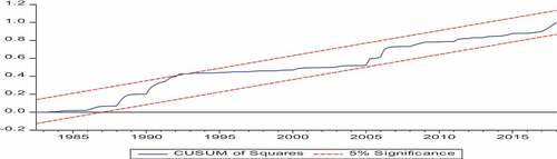
After analyzing the NARDL model and the underlying assumptions’ diagnostics tests, the next step is to use Cumulative Sum of Recursive Residuals (CUSUM) and the Cumulative Sum of Squares (CUSUMQ) tests to assess the stability of the model. The rule of the thumb requires that when the plots lie within the 5% significance level, the model is stable, and the null hypothesis of the model stability cannot be rejected (Bahmani-Oskooee & Fariditavana, 2017). Figure Figure 1 and Figure Figure 2 plot the results of the CUSUM and C.U.S.U.M.S.Q. Tests. The coefficients are stable because the plots of the CUSUM and CUSUMSQ statistics fall inside the critical bands of the 5% confidence intervals of the parameter stability. The plots for each blue line did not cross the red line, the critical value line. Therefore, the coefficients are stable over Ghana’s sample period of study. The model is well specified as a goodness-of-fit to estimate the coefficients of the variables for this study.

Figure 1. Plot of stability test (CUSUM).

The straight line represents critical bounds at 5% significance.

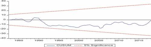
Figure 2. Plot of the stability test (CUSUMQ). Plot of the CUSUM of squares test.

The straight line represents critical bounds at 5% significance

4.7. Dynamic multiplier graph (DMG)

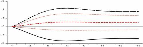
The dynamic multiplier graph (DMG) is used to assess the adjustment of asymmetry in the long-run equilibrium due to the negative change or shock and positive change or shocks in capital flight. The plot for DMG is presented in Figure Figure 3. The DMG in Figure Figure 3 shows the linear mixture of the positive and negative changes in capital flights. The black dash line above in Figure Figure 3 of the DMG shows how economic growth adjusts to the positive change or shock in capital flight, whiles the black line below shows economic growth adjusts to the negative change or shock in capital flight. The small red dash line in the middle is the asymmetric part, and it reflects the difference between the dynamic multiplier of positive and negative changes in capital flight. The asymmetric small red line lies within the upper and lower bounds of the 95% confidence intervals. The result shows that the GDP responds more positively to a positive shock than negatively to a negative shock of capital flight. The outcome from the dynamic multiplier graph confirms the results of the Wald test that the model is stable over the sample period.

Figure 3. Dynamic multiplier graph.

Source: Author’s computation, 2021

5. Conclusion and recommendations

The paper uses the NARDL model as an econometrics tool to investigate the effects of the long-run and short-run relationship between capital flight and economic growth. The result of the ADF test revealed that the series exhibits mixed integration of I(0) and I(1), suggesting the linear ARDL and, by extension, NARDL approach was the most appropriate econometrics tool to assess the effects of capital flight and economic growth nexus. Secondly, the Wald test confirms an asymmetrical relationship between capital flight and economic growth in the short-run and long-run. The error correction term was negative and statistically significant at the 5% level. It means the short-run model restores to long-run equilibrium with time. Furthermore, the findings from the long-run analysis revealed that a 1% change in positive capital flight leads to a decline in economic growth by (0.036), and a 1% change in negative capital flight leads to an increase in economic growth 0.630%. The resultant relationship between positive and negative changes in capital flight and economic growth explains why the capital flight, since 2007, has been accompanied by economic growth. This study then makes essential recommendations based on the evidence from the asymmetric effect of capital flight on economic growth. This result confirms an urgent need for policy to ensure the recovery of all looted public funds by the corrupt public officials stacked in foreign accounts to be retrieved and injected back into the economy of Ghana. There is an urgent need to curb capital flight immediately before it escalates in the future. Government should adopt a conventional tool that strengthens the existing institutions to create conducive opportunities for the investors to redirect funds into the Ghanaian economy. The first limitation of this study is the scarcity and reliability of data availability in developing countries like Ghana. For that matter, the study focused on data from 1977 to 2020. The second limitation is that the study used capital flight (CF), interest rates (I.T.), and inflation (INF) as the only macroeconomic variables. It is also known that economic and political variables affect economic growth. Future research should explore other methodologies, such as hot money methodologies as a measurement of capital flight, and test the asymmetric impact of capital flight on economic growth in other Sub-Saharan economies.

Disclosure statement

No potential conflict of interest was reported by the author(s).

Additional information

Funding

The authors received no direct funding for this research.

References

- Adefeso, H., Egbetunde, T., & Alley, I. (2013). Stock market development and growth in Nigeria: A causal analysis. Arabian Journal of Business and Management Review, 2(6), 78–19. http://dx.doi.org/10.12816/0002295
- Adekunle, W., & Ndukwe, I. (2018). The impact of exchange rate dynamics on agricultural output performance in Nigeria. Munich Personal RePEc Archive.
- Ajayi, I., & Ndikumana, L. (2015). Capital flight from Africa causes effects and policy issues. Oxford University Press.
- Ajilore, T. O. (2015). An economic analysis of capital flight from Nigeria an economic analysis of capital flight from Nigeria. International Journal of Economics and Finance, 2(4), 89–101. https://doi.org/10.5539/ijef.v2n4p89
- Akanbi, O. A. (2015). Structural and Institutional Determinantsof Poverty in Sub-Saharan African Countries. Journal of Human Development and Capabilities, 16(1), 122–141. https://doi.org/10.1080/19452829.2014.985197
- Amu, C. U., Nwezeaku, N. C., & Akujuobi, A. B. C. (2015). Impact of capital market growth on economic growth in Nigeria. American Journal of Marketing Research, 1(3), 93–98. Public Science Framework-Journals - Paper - HTML (aiscience.org)
- Anderl, C., & Caporale, G. M. (2021). Nonlinearities and asymmetric adjustment to PPP in an exchange rate model with inflation expectations. Journal of Economic Studies, 0144-3585, 1–23. https://doi.org/10.1108/JES-02-2021-0109
- Arltova, M. (2016). Statistica. University of Economics.
- Bahmani-Oskooee, M., & Fariditavana, H. (2017). Non-linear ARDL approach, asymmetric effects, and the J-Curve. Journal of Economic Studies, 42(3), 519–530. https://doi.org/10.1108/JES-03-2015-0042
- Bakare, A. S. (2011). The determinants and roles of capital flight in the growth process of the Nigerian economy : Vector autoregressive model approach. British Journal of Management and Economics, 1(2), 100–113. https://journaljemt.com/index.php/JEMT/article/view/30060/56409
- Beja, E. L. (2007). Capital flight and economic performance: Growth projection for the Philippines. Munich Personal RePEc Archive, 2(3), 13–28. https://archium.ateneo.edu/economics-faculty-pubs/140/
- Borio, C. E., English, W. B., & Filardo, A. J. (2003). A tale of two perspectives: Old or new challenges for monetary policy? In BIS Working Papers No (Vol. 127). Bank for International Settlements.
- Boyce, J. K., & Ndikumana, L. (2012). Capital flight from Sub-Saharan African countries: Updated estimate, 1970–2010. Political Economy Research Institute, University of Massachusetts. Retrieved on August 9, 2021, http://www.peri.umass.edu/fileadmin/pdf/ADP/SSAfrica_capitalflight_Oct23_2012.pdf
- Boyd, J. H., Levine, R., & Smith, B. D. (2001). The impact of inflation on financial sector performance. Journal of Monetary Economics, 47(2), 221–248. https://doi.org/10.1016/S0304-3932(01)00049-6
- Bredino, S., Fiderikumo, P., & Adesuji, A. (2018). Impact of capital flight on economic growth in Nigeria: An econometric approach. Journal of Business and Economic Development, 3(1), 22–29. https://doi.org/10.11648/j.jbed.20180301.14
- Byrne, B. M. (2010). Structural equation modeling with A.M.O.S.: Basic concepts, applications, and programming. Routledge.
- Cervena, M. (2006). The Measurement of Capital Flight and Its Impact on Long-Term Economic Growth: Empirical Evidence from a Cross-Section of Countries. Unpublished Master’s thesis, Comenius University Bratislava.
- Cho, J. S., Green-wood-Nimmo, M., & Shin, Y. (2021). Recent developments of the autoregressive distributed lag modelling framework. Journal of Economic Surveys, Special Issue, 1–26. https://doi.org/10.1111/joes.12450
- Davies, V. A. B. (2008). Postwar Capital Flight and Inflation. Journal of Peace Research, 45(4), 519–537. https://doi.org/10.1177/0022343308091359
- Duasa, J. (2007). Determinants of Malaysian trade balance: An ARDL bounds testing approach. Global Economic Review, 36(1), 89–102. https://doi.org/10.1080/12265080701217405
- Eshete, Z. S. (2018). The political economy of capital flight: Governance quality and capital flight in the East Africa community. African and Asian Studies, 49(1), 22–34. https://core.ac.uk/download/pdf/234649306.pdf
- Fisher, R. J. (1993). Social desirability bias and the validity of indirect questioning. The Journal of Consumer Research, 20(2), 303–315.
- Fofack, H., & Ndikumana, L. (2009). Capital flight repatriation: Investigation of its potential gains for Sub- Saharan African countries, World Bank Policy Research Working Paper No. 5024. World Bank Group.
- Fofack, H. (2009). Causality between external debt and capital flight in Sub-Saharan Africa. World Bank Policy Research Working Paper No. 5042, https://ssrn.com/abstract=1471140
- Forson, R., Obeng, C. K., & Brafu-Insaidoo, W. G. (2017). Determinants of capital flight In Ghana. Journal of Business and Enterprise Development, 7(10),104–126. https://papers.ssrn.com/sol3/papers.cfm?abstract_id=2999723
- Gautier, T. T., & Luc, N. N. (2020). Capital flight and economic growth: The case of E.C.C.A.S., E.C.O.W.A.S., and SADC. Countries. The Economic Research Guardian, 10(1), 2–11. https://www.ecrg.ro/files/p2020.10(1)3y1.pdf
- George, D., & Mallery, P. (2010). SPSS for Windows step by step. A simple study guide and reference (10. Baskı) (pp. 10). Boston, MA: GEN.
- Gujarati, D. N., & Porter, D. C. (2009). Basic econometrics (5th ed.). McGraw-Hill Irwin.
- Harswari, M. H. A. B. N., & Hamza, S. M. (2017). The impact of interest rate on economic development: A study on Asian Countries. International Journal of Accounting & Business Management, 5(1), 180–188. doi:10.24924/ijabm/2017.04/v5.iss1/180.188
- Henry, A. W. (2013). Analysis of the effects of capital flight on economic growth: Evidence from Nigerian economy (1980 – 2011). European Journal of Business and Management, 5(17), 21–33. https://core.ac.uk/download/pdf/234624858.pdf
- Hye, Q. M., & Wizarat, S. (2013). Impact of financial liberalization on economic growth: A case study of Pakistan. Asian Economic and Financial Review, 3(2), 270–282. https://citeseerx.ist.psu.edu/viewdoc/download?doi=10.1.1.1090.4231&rep=rep1&type=pdf
- Idris, M., & Baker, R. (2017). Public sector spending and economic growth in Nigeria: In search of a stable relationship. Asian Research Journal of Arts & Social Sciences, 3(2), 1–19. https://doi.org/10.9734/ARJASS/2017/33363
- Irwin, D. A. (2021). How economic ideas led to Taiwan’s shift to export promotion in the 1950s. Peterson Institute for International Economics Working paper, Massachusetts, U.S.A.
- Jao, Y. C. (1976). Trade and economic development in Taiwan. Intereconomics, Verlag Weltarchiv, Hamburg, 11(6), 172–176. https://doi.org/10.1007/BF0292896
- Kadochnikov, D. (2006). Economic impact of capital flight from Russia and its institutional context: Why capital controls cannot be a part of a pro-growth policy (updated version). M.P.R.A. Paper No. 330. Munich Personal RePEc Archive.
- Khalid, M., & Nasir, S. (2004). Saving-investment behaviour in Pakistan: An empirical investigation. Pakistan Development Review, 43(4), 665–682. https://doi.org/10.30541/v43i4IIpp.665-682
- King, R. G., & Levine, R. (1993). Finance and growth: Schumpeter might be right. The Quarterly Journal of Economics, 108(3), 717–737. https://doi.org/10.2307/2118406
- Kline, R. B. (2011). Principles and practice of structural equation modeling (5th ed.). The Guilford Press.
- Lawal, A. I., Kazi, P. K., & Adeoti, O. J. (2017). Capital flight and the economic growth: Evidence from Nigeria. Business Review, 8(1), 125–132. https://doi.org/10.21512/bbr.v8i2.2090
- Lawanson, A. O. (2007). An econometric analysis of capital flight from Nigeria: A portfolio approach. https://opendocs.ids.ac.uk/opendocs/bitstream/item/2944/RP%20166.pdf?sequence=1
- Lucas, R. E., Jr. (1988). On the mechanics of economic development. Journal of Monetary Economics, 22(1), 3–42. https://doi.org/10.1016/0304-3932(88)90168-7
- Makochekanwa, A. (2007). An empirical investigation of capital flight from Zimbabwe. University of Pretoria Working Paper: 2007-11: Department of Economics, University of Pretoria, South Africa. tps://www.up.ac.za/media/shared/61/WP/wp_2007_11.zp39551.pdf
- Mamo, F. T. (2012). Economic Growth and Inflation A panel data analysis. Master of Business Administration (MBA) Thesis Södertörns University.
- Moyo, D., & Munoriyarwa, A. (2021). Data must fall: Mobile data pricing, regulatory paralysis and citizen action in South Africa. Information, Communication & Society, 24(3), 365–380. https://doi.org/10.1080/1369118X.2020.1864003
- Mushtaq, S., & Siddiqui, D. A. (2016). Effect of interest rate on economic performance: Evidence from Islamic and non-Islamic economies. Finance Innov, 2(9), 1–14. https://doi.org/10.1186/s40854-016-0028-7
- Ndiaye, A. S. (2014). Capital flight from the franc zone: Exploring the impact on economic growth. African Economic Research Consortium.
- Ndikumana, L. (2016). Causes and effects of capital flight from Africa: Lessons from case studies. African Development Review, 28(1), 2–7. https://doi.org/10.1111/1467-8268.12177
- Nguena, C. L., & Abimbola, T. M. (2003). Financial deepening dynamics and implication for financial policy coordination in a monetary union: The case of W.A.E.M.U. Article presented at African Economic Conference for Regional Integration in Africa. RePEC: Johannesburg, South Africa.
- Oluwaseyi, M. H. (2017). Capital flight from nigeria: An empirical analysis. Journal of Indonesian Applied Economics, 7(2), 131–145. https://jiae.ub.ac.id/index.php/jiae/article/view/203
- Onodugo, V. A., Kalu, I. E., Anowor, O. F., & Ukweni, N. O. (2014). Is capital flight healthy for Nigerian economic growth? An econometric investigation. Journal of Empirical Economics, 3(1), 10–24. https://ideas.repec.org/a/rss/jnljee/v3i1p2.html
- Orji, A., Ogbuabor, J. E., & Anthony-Orji, O. (2015). Financial liberalization and economic growth in Nigeria: An empirical evidence. International Journal of Economics and Financial Issues, 5(3), 663–672. https://www.econjournals.com/index.php/ijefi/article/view/1284/pdf
- Orji, A., Ogbuabor, E., Kama, K, J., & Anthony-Orjic, O, I. (2020). Capital flight and economic growth in Nigeria: A new evidence from ARDL approach. Asian Development Policy Review, 8(3), 171–184. https://doi.org/10.18488/journal.107.2020.83.171.184
- Osei-Assibey, E., Domfeh, K. O., & Danquah, M. (2018). Corruption, institutions and capital flight: Evidence from Sub-Saharan Africa. Journal of Economic Studies, 45(1), 59–76. https://doi.org/10.1108/JES-10-2016-0212
- Pesaran, M. H., Shin, Y., & Smith, R. J. (2001). Bounds testing approaches to the analysis of level relationships. Journal of Applied Econometrics, 16(3), 289–326. https://doi.org/10.1002/jae.616
- Romer, P. M. (1986). Increasing returns and long-run growth. The Journal of Political Economy, 94(5), 1002–1037. https://www.jstor.org/stable/1833190#metadata_info_tab_contents
- Romer, P. M. (1994). The origins of Endogenous growth. Journal of Economic Perspectives, 8(1), 3–22. https://doi.org/10.1257/jep.8.1.3
- Salahuddin, M., & Gow, J. (2009). The relationship between economic growth and remittances In the presence of cross-sectional dependence. Journal of Developing Areas, 49(1), 207–221. https://doi.org/10.1353/jda.2015.0007
- Shin, Y., Yu, B., & Greenwood-Nimmo, M. (2014). Modeling asymmetric co-integration and dynamic multipliers in a Non-linear ARDL Framework. S.S.R.N. Electronic Journal, 1–61. https://doi.org/10.2139/ssrn.1807745
- Shrestha, M. B., & Bhatta, G. R. (2018). Selecting appropriate methodological framework for time series data analysis. Journal of Finance and Data Science, 4(2), 71–89. https://doi.org/10.1016/j.jfds.2017.11.001
- Swarnapali, R. (2014). Firm specific determinants and financial performance of licensed commercial banks in Sri Lanka. Paper presented at the International Conference on Management and Economics, University of Ruhuna, Sri Lanka.
- Tjaondjo, C. N. (2019). Determinants of capital flight in Namibia. Unpublished Master’s dissertation, Graduate School of Business. http://hdl.handle.net/11427/30583
- Vu, Q., & Zak, P. J. (2006). Political risk and capital flight. Journal of International Money and Finance, 25(25), 308–329. https://doi.org/10.1016/j.jimonfin.2005.11.001
- Walter, I. (1987). The mechanisms of capital flight. In D. R. Lessard & Williamson (Eds.), Capital flight and third world debt. Institute of International Economics, 103–128.
- The World Bank, World Development Indicators (2021). GDP, Capital flight, [DataBank]. https://databank.worldbank.org/reports.aspx?source=world-development-indicators
- Zheng, Y., & Tang, K. (2009). Rethinking the measurement of capital flight: An application to Asian economies. Journal of the Asia Pacific Economy, 14(1), 313–330. https://doi.org/10.1080/13547860903169308