The performance of zero-cost option derivative strategies during turbulent market conditions in developing and developed countries

Abstract

Financial markets behave in a volatile manner at certain stages in their maturity. These volatile conditions pose a market risk to an investor that can be limited by imposing derivatives strategies within the investment objective. The aim of this paper is to provide investors with a trading strategy to effectively manage turbulent market conditions (such as during the Covid-19 pandemic) by implementing a strategy that has a continuous approach of implementation. The study chose to include three main turbulent market periods such as the Dotcom bubble (1995–2005), the financial crisis (2008–2009), and more recently the COVID-19 pandemic (2020). Stock indices from six different stock exchange countries were chosen for comparison (also aligned to different geographical locations and developing versus developed economies) who were most likely to be affected by the extreme market events. Zero-cost collars are option-based strategies that can be used by investors to provide costless protection for stock or index investment. This strategy is obtained by setting equal the price obtained and the price paid for the components of the strategy. Previous literature has to date, not explored the potential outcomes for such procedures of different frequency intervals and the effect thereof on the performance in turbulent and non-turbulent market conditions. It was observed that moderate levels of market volatility combined with high-performing indices provide the scenario for the zero-cost collar to result in respectable returns. Furthermore, in order to add to this performance the strike level of the put option contract needs to be increased. Consequently, respectable results will be produced during periods of both significant market downturns.

Keywords:

• option contracts
• derivative strategies
• zero-cost collar
• market volatility
• COVID-19

1. Introduction

Financial market volatility is seen as an indication of the rate of change, among other things, of security prices over a specified time horizon. Although volatility poses a considerable market risk to investors, it may be mitigated through the application of trading strategies (Krauss, 2017). Different market conditions (which arise for example, from different jurisdictions, such as developed versus emerging economies or epochs, such as benign turbulent and non-turbulent market periods which again influences volatility consideration for an investor) result in different strategy effectiveness (in turbulent and non-turbulent market conditions), which is little understood. It would be to the benefit of the investor to understand and explore further technical methods (framework of implementation) and techniques (performance measurement) on trading strategies, which are trigger-based (derivative strategy triggered or indicated by fractal dimensions) or continuous implementation (derivative strategy implemented on a rolling basis) to complement and adhere to the investor objectives. This addition will bring about a broader aspect of trading strategy implementation to the investor of implementing and using certain strategy construction or consideration over the investment horizon.

Therefore, the research question of this article is to analyse what the most effective manner is in which a derivative strategy should be applied to volatile market conditions to hedge an investor’s market risk and obtain adequate strategy performance. The existing theory will help determine the viability of derivative strategy implementation (continuous implementation of the zero-cost strategy) use across different dynamics (such as developing versus developed countries, different indices, and different maturity and strike price levels).

Therefore, the aim of this paper is to provide investors with a trading strategy to effectively manage turbulent market conditions (such as during the Covid-19 pandemic) by implementing a strategy that has a continuous approach of implementation. The study chose to include three main turbulent market periods such as the Dotcom bubble (1995–2005), the financial crisis (2008–2009), and more recently the COVID-19 pandemic (2020). In terms of the empirical contribution of this article, it involved the implemented a preselected framework of a trading strategy on selected economies (developed economies—USA (S&P500), China (Nikkei 225), and United Kingdom (FTSE 100), developing economies (South Africa (JSE ALSI), Brazil (BOVESPA), and Russia (RTSI)). As well as implemented a continuously applied trading strategy on developing as well as developed economies (developed economies—USA (S&P500), China (Nikkei 225) and United Kingdom (FTSE 100), developing economies (South Africa (JSE ALSI), Brazil (BOVESPA), and Russia (RTSI)). Furthermore, tested whether cost-efficient derivative strategies meet investors’ profitability objectives over specific time horizons of expiry for the option contracts (such as 3 -, 6—and 9-month expiration periods). And lastly, built a the cost-efficient model—tested the model’s output on various indices (as a proxy) and compared the performance within selected economies.

This paper will therefore aim to provide a better understanding of the performance by implementing multiple levels of maturity and strike price levels of rolling zero-cost collars influenced by the prevailing market conditions. This in turn will contribute towards the understanding of the dynamics of the strategies. The principal variables are put strike percentages, which are user-defined in practice and are used in the zero-cost collar to balance associated call strikes so that the applied strategy incurs no costs.

2. Literature review

Prevailing market conditions dictate the performance of investors and their applicable strategies on the market. An investor could find it difficult to navigate the prevailing market conditions according to their risk tolerance and return objectives. An investor has the ability to implement a trading strategy to assist with managing these parameters within the prevailing market conditions and contribute to their investment objectives. The investor can make use of option derivative contracts simultaneously with their underlying asset holding. The concept of a cost-efficient derivative strategy is obtained by imposing a combination of the sale of a derivative (could be multiple) and simultaneously buying another derivative (could also be multiple) to protect gains of the asset and limit the downside risk of the investment. By setting up the derivative strategy in such a manner will effectively produce a scenario where the investor will not pay for the implementation of the application strategy. The most important factors in pricing the applicable derivative strategies are calculated using the Black and Scholes model (Black & Scholes, 1973) and are implemented in such a manner with preselected investment objectives that will make the application of a cost-efficient derivative strategy possible.

Relating to investment objectives for the investor, the risk appetite or risk tolerance level greatly determines the minimum loss (floor cap) by selecting a relevant put option strike level, which then influences the associated call option strike level. The call option price is obtained by means of reverse engineering from the call option value, which in return establishes the strategy maximum return level (Dubil, 2010). By increasing or decreasing the floor value of the strategy would also then increase the cap or maximum return and vice versa. Rolling strategies involve the purchase and later sale of the derivative components at a chosen frequency for the investor (Chen, 2007).

A Zero-cost collar (ZCC) is a derivative strategy that simultaneously implements (buy or sell of an option contract) a put and a call option to protect a stock (or equity index) by limiting upside and downside risk associated with the investor (Yim et al., 2011). The price of these options (bought and sold) is therefore implemented to be equal at the time of implementation and as a result, this form of collar strategy is effectively costless to the investor (Bartoňová, 2012). A zero-cost collar comprises mainly of options contracts which is a cost-efficient way to protect stock gains by limiting potential losses. The strategy, which comprises the simultaneous purchase of a put option and sale of a call option, provides the call option purchaser with the right to purchase a given underlying asset at a set price while, to restrict losses, the put option limits the risk of a decrease in value with a floor under the current price of the stock (Duff, 1997). Zero-cost collars provide an efficient strategy for bullish investors. The put option strike level is, therefore, usually set first, depending on the investor’s risk tolerance according to their investment objectives, then the call option strike price is calculated in a manner to generate enough value for the put option purchase. This option-based strategy allows investors to hedge their investment while still maintaining profit potential and also renders the entire transaction cost-free to the investor (Gordon, 2015).

Rolling zero-cost collars comprise numerous individual zero-cost collars, implemented consecutively at a chosen frequency by the investor (Lui & Mole, 1998). Such strategies are constructed with the same maturity and time to expiry, so, for example, a three-month zero-cost collar could be purchased each subsequent month and at the end of the first three-month period, the first collar is closed, then the second collar closed one month later, and so on (Ahn et al., 2003). The performance of the zero-cost collar is then determined when compared to a relevant market index by using the returns generated from the strategy (Cuoco et al., 2008).

This method of putting a financial product together or contract can be used as a risk management tool from the perspective of the investor to limit his downside risk, by having the ability to sell a declined asset’s price at a higher value (Bunch & Johnson, 2000). A put option contract also has limiting dynamics where the maturity of the long put contract is agreed upon by the seller and purchaser (Witzany, 2020). The longer the agreed maturity (usually in monthly cycles) the more the purchaser will pay in premium for his agreement of the contract (Merton, 1972).

The collar derivative strategy is obtained by combining the three named elements or dynamics (Israelov & Klein, 2016). The cost implications that the option contract holds for the speculator is irrelevant to him as a result of the combination that produces a return that the cost of selling the call option contract will pay for the cost of purchasing the put option contract (El-Hassan et al., 2018). By implementing the derivative strategy in this manner, a collar is produced that will ultimately limit the losses (downside risks) below the put option contract strike price to the loss from the initial stock price to that strike price, which is observed to be the floor of the derivative strategy (Israelov & Klein, 2017).

Since the mechanism for constructing a ZCC is effectively costless to the investor, there is, however, an aspect of opportunity cost where profit or gains with the ZCC is forgone (Bartoňová, 2012). Another element with the ZCC strategy is to essentially implement on market timing where the duration (maturity length on both long put and short call option contracts) also needs to be selected by the investor depending on the applicable risk tolerance. Effectively choosing a too short or too long duration of maturity (as input into put- and call option pricing) could have a potential profit or gain implications as well to the investor (Rekha, 2019).

3. Data and methodology

3.1. Data

The data used in this article span over 26 years from January 1995 to December 2020. This period was chosen to include three main turbulent market periods such as the Dotcom bubble (1995–2005), the financial crisis (2008–2009), and more recently the COVID-19 pandemic (2020). Stock indices from six different stock exchange countries were chosen for comparison (also aligned to different geographical locations and developing versus developed economies). The data allowed for the Implemented a preselected framework of a trading strategy on selected economies (developed economies—USA (S&P500), China (Nikkei 225), and United Kingdom (FTSE 100), developing economies (South Africa (JSE ALSI), Brazil (BOVESPA), and Russia (RTSI)). As well as implemented a continuously applied trading strategy on developing as well as developed economies (developed economies—USA (S&P500), China (Nikkei 225) and United Kingdom (FTSE 100), developing economies (South Africa (JSE ALSI), Brazil (BOVESPA), and Russia (RTSI)). Furthermore, tested whether cost-efficient derivative strategies meet investors’ profitability objectives over specific time horizons of expiry for the option contracts (such as 3 -, 6—and 9-month expiration periods). And lastly, built a cost-efficient model—tested the model’s output on various indices (as a proxy) and compared the performance within selected economies.

These indices were specifically chosen to provide a representation of developed and emerging markets across different geographical locations across the globe. This diversification also aligns to the theoretical object of obtaining the viability of option derivative strategy implementation use across different dynamics (such as developing versus developed countries, different indices and different maturity and strike price levels).

3.1.1. Developed economies

• Standard & Poor’s 500 is a United States-based index fund that comprises the 500 largest companies, weighted by factors such as size and liquidity, on the New York Stock Exchange (Ongom et al., 2021). Standard & Poor’s 500 is widely considered to be the best representation of the US stock market.

• The NIKKEI 225 (Nikkei Stock Average): A Japanese index comprising 225 large companies, weighted by factors such as price and performance of the 225 largest companies traded on the Tokyo Stock Exchange across a wide variety of sectors in the Tokyo financial markets. The NIKKEI 225 is widely considered to be the best representation of the Asian stock market (Montshioa et al., 2021).

• The Financial Times Actuaries 100 Index is a United Kingdom-based index fund comprising 100 blue-chip stocks that are listed on the London Stock Exchange. The London Stock Exchange is the second-largest stock exchange in Europe by market capitalisation and is commonly used as the UK and global equity benchmark (Montshioa et al., 2021).

3.1.2. Developing economies

• The Johannesburg Stock Exchange All Share Index is a South African-based equity index fund comprised the top-listed companies weighted by factors such as size and liquidity in South Africa. The Johannesburg Stock Exchange is the 19th largest stock exchange and largest by market capitalisation in Africa.

• The BOVESPA (IBOVESPA): A Brazilian equity index representing the majority of trading and market capitalisation on the Brazilian Stock Exchange (Ongom et al., 2021). This index is measured by 70 public-traded companies on the B3 (Brazil Stock Exchange and over-the-counter market). This index is a weighted measurement and is a fair representation of the South American financial markets being listed as the 13^th largest stock exchange in the world.

• The Russian Trading System Index (RTSI): A Russian equity index comprised 50 Russian public stocks traded on the Moscow exchange (Kuramshina, 2021). This is a free-float index calculated by capitalisation-weighted measurement on a three-month review basis.

3.2. Methodology

The volatility model was implemented using the exponential weighted moving average (EWMA) (one of the input variables to calculate the price of an option contract) is calculated using the implied EWMA volatility of the respective volatility indices. Furthermore, regarding the developed economies, the Chicago Board Options Exchange (CBOE) volatility Index (VIX) was used for the US index, for the Japanese Index the volatility index Japan (VXJ) was used and lastly, for the United Kingdom (UK) index the FTSE implied volatility index series (IVI) was used. In terms of the developing economies, the JSE’s South African Volatility Index (SAVI) which is modelled on the VIX was used (JSE, 2020). The Chicago Board Options Exchange Brazil ETF volatility index was used for the Brazilian index and for the Russian index the Russian Volatility Index (RVI) was used. Table 1 describes the applicable volatile index used for each geographical index.

Table 1. Volatility modelled index summary

Index	Name	Volatility Index used	Developed/Developing economy
S&P 500	Standard & Poor’s 500	Chicago Board Options Exchange Volatility Index	Developed
NIKKEI 225	Nikkei Stock Average	Volatility Index Japan	Developed
FTSE 100	Financial Times Actuaries 100 Index	Implied Volatility Index Series	Developed
JSE ALSI	Johannesburg Stock Exchange All Share Index	South African Volatility Index	Developing
BOVESPA	IBOVESPA	Chicago Board Options Exchange Brazil ETF Volatility Index	Developing
RTSI	Russian Trading System Index	Russian Volatility Index	Developing

Source: Author compilation

The daily average dividend yields (one of the key components of an option price) were obtained from the respective index data providers. Risk-free rates used are those most commonly used in the countries where the index is hosted as can be seen in Table 2. The six risk-free rates used for the six indices are those in the United Kingdom, the three-month London Interbank Offer Rate (LIBOR), Federal Funds Rate for the S&P500 in the United States, the Japan Government Bond 10-year bond rate for the Japanese index (NIKKEI225), the Johannesburg Interbank Agreed Rate (JIBAR) in South Africa, the Brazil Government Bond 10-year bond rate for the Brazilian index (BOVESPA) and the Russia Government Bond 10-year bond rate for the Russian index (RTSI).

Table 2. Risk-free rate index summary

Index	Name	Risk-free rate used
S&P 500	Standard & Poor’s 500	Federal Funds Rate
NIKKEI 225	Nikkei Stock Average	Japan Government Bond 10-year bond rate
FTSE 100	Financial Times Actuaries 100 Index	London Interbank Offer Rate
JSE ALSI	Johannesburg Stock Exchange All Share Index	Johannesburg Interbank Agreed Rate
BOVESPA	IBOVESPA	Brazil Government Bond 10-year bond rate
RTSI	Russian Trading System Index	Russia Government Bond 10-year bond rate

All options’ maturities ($T$), were initially set to three months for comparison. Other maturities (three, six or nine months) are possible in principle but are uncommon in practice (Bartoňová, 2012).

Dividends earned by holding the underlying stock (or in an index) affect applicable option prices. In order to account for this, dividends are removed from the index level (as indicated by equation (1)(1) $I=S_0\cdot \alpha e^{-rT}$(1) ), $S_0$, as an investment. This amount is calculated using:

(1) $I=S_0\cdot \alpha e^{-rT}$(1)

where $\alpha$ is the dividend percentage. This depreciates the value of the dividend, paid at maturity, to the commencement date of the option, which is then subtracted from the stock index price, $S_0$. Next, the nominal index values were calculated for each index separately to give comparable, standardised representations, using $S_t/S_0$ where $S_t$ is the current stock price and $S_0$ is the initial index price.

For the Zero-cost collar strategy, the investor risk tolerance is represented by the put option strike price, $K_p$, which can also be adjusted by choosing $\theta$ (a percentage below the index price, $S_0$) using $K_p=S_0\cdot \left(1-\theta \right)$. If an investor chose the put option strike price (according to their risk tolerance) at the value of 5% below the index price and the index price is currently at 100, then the strike price denoted by $\theta$, is $95\mathrm{\%}\times 100=95$. For this paper, a variety of possible values, representing different risk tolerance levels, were selected to create a variety of risk tolerance levels and their respective performance.

Call and put option prices for the applicable derivative strategy were calculated using (respectively):

(2) $c=S_{0}N{d}_1-K_c{e}^{-rT}N{d}_2$(2)

and

(3) $p=K_p{e}^{-rT}N-d_2-S_{0}N-d_1$(3)

where $c$ is the call price (equation 2(2) $c=S_{0}N{d}_1-K_c{e}^{-rT}N{d}_2$(2) ), $p$ is the put price (equation 3(3) $p=K_p{e}^{-rT}N-d_2-S_{0}N-d_1$(3) ), $S_0$ is the stock price, $K_c$ is the strike price of the call, $K_p$ is the strike price of the put, $r$ is the risk-free rate of return, $T$ is the time to expiration, $N\left(x\right)$ is the normal distribution of the value for $x$, and $d_1$ (equation (4)(4) $d_1=\frac{lnln(\frac{S_0}{K)+(r+\frac{{\sigma }^2}{2)T}}}{\sigma \sqrt{T}}$(4) ) and $d_2$ (equation (5)(5) $d_2=\frac{lnln(\frac{S_0}{K)+(r-\frac{{\sigma }^2}{2)T}}}{\sigma \sqrt{T}}=d_1-\sigma \sqrt{T}$(5) ) are given by:

(4) $d_1=\frac{lnln(\frac{S_0}{K)+(r+\frac{{\sigma }^2}{2)T}}}{\sigma \sqrt{T}}$(4)

and

(5) $d_2=\frac{lnln(\frac{S_0}{K)+(r-\frac{{\sigma }^2}{2)T}}}{\sigma \sqrt{T}}=d_1-\sigma \sqrt{T}$(5)

where $K$ is the strike price for the put option contract or call option contract depending on which is being calculated, $\sigma$ is the volatility of the stock (Black & Scholes, 1973). Note that for the zero-cost collar strategy, $T=3$ months and $S_0,\sigma$, $r,$ and $\alpha$ are obtained from historical data. $K_p$ is dependent on the variable $\theta$, which is adjusted for various values to ascertain the effect of the put strike level and for the strategy’s performance. The call option price is then calculated using equation (4)(4) $d_1=\frac{lnln(\frac{S_0}{K)+(r+\frac{{\sigma }^2}{2)T}}}{\sigma \sqrt{T}}$(4) and a value of $K_c$ which sets $c=p$. The minimum or floor return and maximum return (cap) and strategy returns for the zero-cost collar are summarised in Table 3.

Table 3. Summary of strategy returns

	ZCC
Floor return	$-\theta$
Cap return	$K_c-S_0{S}_0$
Strategy return	In the range $K_p\le I\le K_c$ the return is $I-S_0{S}_0$

4. Results

The 26 years chosen for this analysis were characterised by both highly turbulent periods dominated by the dot-com bubble (1995–2005), the financial crisis in 2008/9 and more recently the COVID-19 pandemic in 2020 as well as a period of relatively non-volatile growth as shown in Figure 1.

Figure 1. Relative performance of the six indices from January 1995 to December 2020.

The performance of the indices in question varies considerably indicated by end-of-term values in Figure 1. The RTSI and the BOVESPA indices grew the strongest before the dot-com bubble (end of 2005) and were least affected by this market period. The JSE ALSI, when compared to the rest of the indices, also performed relatively well during this period of turbulent market conditions. All three of these indices are categorised as developing economy indices and were least affected by the dot-com bubble relative to the developed economies. Post this period, the developing economy indices growth continued. Following this growth spurt, all the indices’ performance was influenced by the financial crisis of 2008/9, the developing economies losing most of their performance gained between 2005 and 2008, the RTSI was most affected in terms of performance during this period.

The S&P 500 (developed economy) and JSE ALSI (developing economy) have proven to show robust growth over the full period but more so since the financial crisis. Both indices have trebled in value since January 2009 and continue this growth until the end of the chosen period. The NIKKEI 225 and the FTSE 100 have not increased much over the full period, ending the period only 39% up and 114% up, respectively, since January 1995 relative to the other indices. The COVID-19 pandemic of 2020ʹs influence can be noted in Figure 1 for all the indices in question, but relative to the two previous turbulent market conditions, the indices have regained their performance track. All the indices under analysis have been influenced by the named three turbulent market conditions and the effects thereof, but from a pure performance measurement perspective, the developing economies have been least affected by the market conditions considering their volatile performance movement.

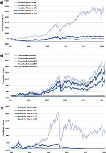
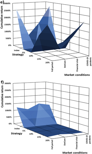
The performance of the zero-cost collar trading strategy was then examined, for each index, over the full period. Figure 2 (a,b,c) shows the cumulative returns of the Zero-cost collar strategy (with $K_p$= 5 percent) with the BOVESPA (a), JSE ALSI (b) and RTSI (c) index as underlying indices representing the developing economies. The level of market volatility was 7%—(a), 4%—(b) and 8%—(c) respectively. Figure 3.2 (d,e,f) shows the cumulative returns of the zero-cost collar strategy (with $K_p$= 5%) with the FTSE100 (d), NIKKEI 225 (e), and S&P 500 (f) index as underlying indices representing the developed economies. The level of market volatility was relatively lower than the volatility for the developing economies with 4%—(d), 5%—(e), and 4%—(f).

Figure 2. (a,b,c): Relative performance of the six developing economies indices from January 1995 to December 2020. (d,e,f): Relative performance of the six developed economies indices from January 1995 to December 2020.

Figure 2. Continued.

Comparing the results of the different indices gave similar results to the relative performance of the indices in Figure 1, where it was observed that the developing economies relatively outperformed the developed economies. The developed economies, however, showed resilient performance over the full period with consistent growth and less volatile movements. It is observed that the arbitrary number of $K_p$= 5%, for the put strike price implemented for the zero-cost collar trading strategy (an indication of the investors’ risk tolerance), produces a return closely correlated to the performance of each index depicted in Figure 2(a,b,c) and Figure 2(d,e,f). This level of risk tolerance is relatively low and it is difficult for the zero-cost collar trading strategy to take advantage of the performance produced by the indices in periods of relative growth, the zero-cost collar strategy being capped at 5%. It is also observed in Figure 2(f) —for the S&P 500—for the period of 1995 to 2008, the zero-cost collar outperforms the index over this period.

The zero-cost collar option derivative strategy’s performance increases in the performance for some indices as the put option contract strike level is increased (increasing the call option strike level as well). When relatively lower levels of $K_p$ is chosen, $K_c$ produces a similar effect in terms of performance and although the strategy is protected against a price decrease, the investor cannot enjoy relatively high returns to the underlying index when the market does improve in terms of performance. Therefore, although the 5 percent strike zero-cost collar strategy in Figures 3(a—f) is protected from the turbulent market conditions of the dot-com bubble, financial crisis, and COVID-19 pandemic the outperformance never materialises as losses accumulate after the crisis with no associated index growth. However, for the indices of the S&P 500 (Figure 3(a)) and NIKKEI 225 (Figure 3(b)) as the put option strike price is increased, the option derivative strategy improves in terms of performance until it even produces results where it outperforms the underlying index. This is principally due to that such an option derivative strategy was protected from the full impact of the named turbulent market conditions (dot-com bubble, financial crisis, and COVID-19 pandemic) and then took advantage of the strategies’ mechanism to take advantage of upside market conditions. In the case of the other four indices, the cumulative performance of the option derivative strategy increases as the put option strike price is increased, but is not enough to outperform the underlying index. This is principally due to that such an option derivative strategy was not protected from the full impact of the turbulent market conditions and could not take advantage of upside market performance, but rather was influenced by decreasing market behaviour. Note that eventually, when $K_p$ is as large as the worst monthly return registered in turbulent market conditions, the zero-cost collar strategy will mimic the index exactly.

Figure 3. (a): Cumulative returns of the S&P 500 Index and increasing put option strike prices. (b): Cumulative returns of the NIKKEI 225 Index and increasing put option strike prices. (c): Cumulative returns of the FTSE 100 Index and increasing put option strike prices. (d): Cumulative returns of the JSE ALSI Index and increasing put option strike prices. (e): Cumulative returns of the BOVESPA Index and increasing put option strike prices. (f): Cumulative returns of the RTSI Index and increasing put option strike prices.

Source: Author compilation

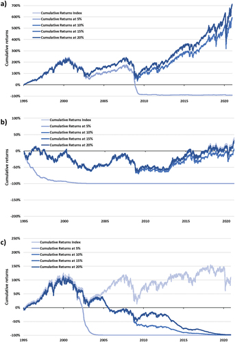
Figure 3. Continued.

Next, the paper explores the volatility of the zero-cost collar strategy, implemented on each chosen index, during certain time periods (turbulent market conditions) and over the full period. Figure 4 (a—f) and Figure 5 (a—f) were produced by calculating the zero-cost collar strategy performance during the specific turbulent market conditions and for over various put option strike levels, at different market volatility levels, $\sigma ,$ and cumulative returns. The $\sigma$ levels are subjective and dependent upon the measurement technique used when pricing the applicable derivative option contract, as it is one of the key components in this paper, it was exponentially weighted moving average as mentioned before to the effect that these values are not directly observed in the market.

Figure 4. (a): Volatility levels for the ZCC implemented on the S&P 500 indices as underlying, as a function of put option strike levels and turbulent market conditions. (b): Volatility levels for the ZCC implemented on the NIKKEI 225 as underlying, as a function of put option strike levels and turbulent market conditions. (c): Volatility levels for the ZCC implemented on the FTSE 100 indices as underlying, as a function of put option strike levels and turbulent market conditions. (d): Volatility levels for the ZCC implemented on the JSE ALSI indices as underlying, as a function of put option strike levels and turbulent market conditions. (e): Volatility levels for the ZCC implemented on the BOVESPA as underlying, as a function of put option strike levels and turbulent market conditions. (f): Volatility levels for the ZCC implemented on the RTSI indices as underlying, as a function of put option strike levels and turbulent market conditions.

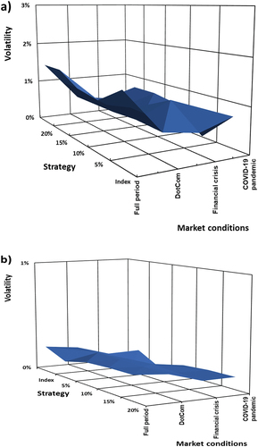
Figure 4. Continued.

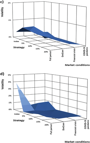
Figure 4. Continued.

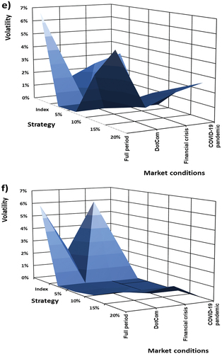
Figure 5. (a): Cumulative return as a function of put option strike levels and turbulent market conditions on the S&P 500. (b): Cumulative return as a function of put option strike levels and turbulent market conditions on the NIKKEI 225. (c): Cumulative return as a function of put option strike levels and turbulent market conditions on the FTSE 100. (d): Cumulative, as a function of put option strike levels and turbulent market conditions on the JSE ALSI. (e): Cumulative, as a function of put option strike levels and turbulent market conditions on the BOVESPA. (f): Cumulative, as a function of put option strike levels and turbulent market conditions on the RTSI.

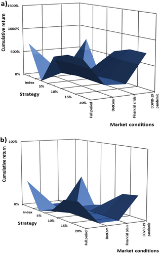
Figure 5. Continued.

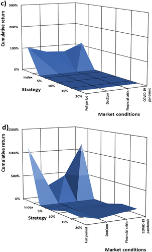
Figure 5. Continued.

Figures 5 (a–f) shows the zero-cost collar strategy cumulative performance for each index measured over different levels of or put option strike levels or $K_p$ and implemented on the prevailing market conditions. Note that the cumulative return for the strategy and the volatility level (vertical axis) scale is the same for both Figures 4 (a–f) and Figures 5 (a–f) for ease of comparison. The zero-cost collar strategy’s volatility or risk taken is affected by increasing levels for $\sigma$, for the S&P 500 (a), NIKKEI 225 (b), FTSE 100 (c), and BOVESPA (e) indices. For these indices increasing levels of $K_p$, the volatility levels increase steeply than at a diminishing rate over the turbulent market conditions. For $K_p=20$%, the zero-cost collar strategy’s performance produces the highest levels of volatility for each index and for $K_p=5$% produces the lowest levels of volatility for the strategy.

The zero-cost collar strategy’s cumulative return performance (Figures 5) is affected by increasing levels for $\sigma$, for the S&P 500 (a), NIKKEI 225 (b), and BOVESPA (e) indices. For these indices increasing levels of $K_p$, the cumulative return performance increases relative to that of the underlying index. For $K_p=20\mathrm{\%}$, the ZCC strategy’s performance produces the highest levels of cumulative return for each index and for $K_p=5\mathrm{\%}$ produces the lowest levels of volatility for the strategy. Comparing strategy performance in turbulent market conditions the effect of higher volatility levels and increased levels for $K_p$. The cumulative return during the dot-com bubble market condition affected each index least, except for the BOVESPA Index (Figure 5 (e)) where the index had its worst market condition performance. The effect of the financial crisis had the biggest impact on the underlying indices’ performance where the lowest cumulative return was recorded, the higher levels of market volatility attributed to this performance. The most recent turbulent market condition of the COVID-19 pandemic had the least effect on the strategies performance, the only measure of a year (Ibovespa, 2020), the strategy is able over each level of $K_p$ to produce relative higher returns relative to the underlying index.

The FTSE 100 (c) and JSE ALSI (d) indices fared worse than that of the S&P 500 and NIKKEI 225 in all market conditions. Being one of the developed economies under analysis the FTSE suffered severe losses during the financial crisis and COVID-19 pandemic, but not as badly as when compared to the S&P 500 and Chinese index of the NIKKEI 225, the other developed economies. This explains the sluggish performance during each prevailing turbulent market condition. Post the financial crisis, the United Kingdom suffered two significant setbacks in the form of the European sovereign crisis of 2011 and also, the Brexit vote in mid-2016. This event, from which the United Kingdom has still not in 2018 fully recovered and resulted in unimpressive comparative performance post this turbulent market condition.

During the turbulent market conditions, the zero-cost collar strategy using the S&P 500 as underlying produced mediocre cumulative returns—in terms of volatility as a function of prevailing market conditions and increasing levels of $K_p$, as the index suffered the worst losses in comparison with all other market indices. This explains the poor strategy performance in Figure 5 (a). The US market fared well post-financial crisis and was not much affected by external market conditions.

The ZCC strategy performance for the BOVESPA Index was like that of the S&P 500. The BOVESPA performed well with the associated ZCC strategy performance relative to other indices. The RTSI also produced results to that of the BOVESPA Index. The overall results are summarised in Table 4 (DotCom bubble), Table 5 (financial crisis), and Table 6 (COVID-19 pandemic).

Table 4. Summary of ZCC strategy statistics and performance in the Dotcom bubble

UI	Market conditions (1995–2005)			ZCC
	$\sigma$	$r_c$	Environment
S&P 500	$5,8\%$	$177\%$	• Moderate $\sigma$, moderate growth • Losses due to DC but small compared with other developed economies	• $-0,27\%r_c+235\%$ • Increases for $K_p+5\%$
NIKKEI 225	$2\%$	$-17\%$	• Low $\sigma$, negative growth • Largest losses due to DC • Overall loss due to low $\sigma$	• $-62\%r_c+15\%$ • Worst performer $\forall K_p$ • Flat for $K_{p}5\%$
FTSE 100	$3,2\%$	$85\%$	• Low $\sigma$, moderate growth • Moderate losses due to DC	• $-4\%r_c+125\%$ • Flat for $K_{p}5\%$
BOVESPA	$16\%$	$683\%$	• High $\sigma$, high growth • Losses due to DC but small compared with other developing economies	• $-50\%r_c+686\%$ • Second best performer $\forall K_p$ • Flat for $K_{p}5\%$
JSE ALSI	$5,8\%$	$280\%$	• Moderate $\sigma$, moderate growth	• $-12\%r_c+280\%$ • Third best performer $\forall K_p$ • Increases for $K_{p}10\%$
RTSI	$23,4\%$	$1095\%$	• High $\sigma$, high growth • Losses due to DC but small compared with other developing economies	• $-62\%r_c+1094\%$ • Best performer $\forall K_p$ • Flat for $K_{p}5\%$

UI underlying index

DC dot-com bubble of 1995–2005

$r_c$ cumulative return

Table 5. Summary of ZCC strategy statistics and performance in the financial crisis

UI	Market conditions (2008/2009)			ZCC
	$\sigma$	$r_c$	Environment
S&P 500	$4,6\%$	$147\%$	• Moderate $\sigma$, moderate growth • Losses due to FC but small compared with other developed economies	• $47\%r_c+215percent$ • Increases for $K_p+10\%$
NIKKEI 225	$1,1\%$	$-47\%$	• Low $\sigma$, negative growth • Largest losses due to FC • Overall loss due to low $\sigma$	• $-64\%r_c-25\%$ • Worst performer $\forall K_p$ • Increases for $K_{p}10\%$
FTSE 100	$2,4\%$	$79\%$	• Low $\sigma$, moderate growth • Moderate losses due to FC	• $14\%r_c+110\%$ • Increases for $K_{p}5\%$
BOVESPA	$26\%$	$1540\%$	• High $\sigma$, high growth • Losses due to FC but small compared with other developing economies	• $588\%r_c+1621\%$ • Best performer $\forall K_p$ • Flat for $K_{p}5\%$
JSE ALSI	$8,2\%$	$477\%$	• Moderate $\sigma$, high growth • Losses due to FC but small compared with other developing economies	• $266\%r_c+589\%$ • Third best performer $\forall K_p$ • Flat for $K_p>5\%$
RTSI	$61\%$	$1455\%$	• High $\sigma$, high growth • Losses due to FC but small compared with other developing economies	• $389\%r_c+2397\%$ • Second best performer $\forall K_p$ • Flat for $K_{p}5\%$

UIunderlying index

FCfinancial crisis of 2008/9

$r_c$cumulative return.

Source: Author compilation

Table 6. Summary of ZCC strategy statistics and performance in the COVID-19 pandemic

UI	Market conditions (2008/2009)			ZCC
	$\sigma$	$r_c$	Environment
S&P 500	$7\%$	$714\%$	• Moderate $\sigma$, high growth • Losses due to C-19 but small compared with other developed economies	• $+388\%r_c+716\%$ • Increases for $K_p>+5\%$
NIKKEI 225	$1,2\%$	$40\%$	• Low $\sigma$, low growth • Largest losses due to C-19	• $-16\%r_c+40\%$ Worst performer $\forall K_p$ • Increases for $K_{p}5\%$
FTSE 100	$7\%$	$113\%$	• Low $\sigma$, moderate growth • Moderate losses due to C-19	• $+62\%r_c+149\%$ • Flat for $K_{p}5\%$
BOVESPA	$32\%$	$2711\%$	• High $\sigma$, high growth • Losses due to C-19 but small compared with other developing economies	• $+1395\%r_c+2711\%$ • Best performer $\forall K_p$ • Flat for $K_{p}5\%$
JSE ALSI	$9,2\%$	$1140\%$	• Moderate $\sigma$, high growth • Losses due to C-19 but small compared with other developing economies	• $+689\%r_c+1158\%$ • Third best performer $\forall K_p$ • Increases for $K_{p}10\%$
RTSI	$16,3\%$	$1296\%$	• High $\sigma$, high growth • Losses due to C-19 but small compared with other developing economies	• $+730\%r_c+1543\%$ • Second best performer $\forall K_p$ • Flat for $K_{p}5\%$

UI underlying index

C-19 COVID-19 pandemic of 2020.

$r_c$ cumulative return.

5. Conclusion and recommendations

This paper explored the performance of a continuously implemented option derivative strategy, zero-cost collar, under both turbulent and non-turbulent market conditions in different geographies and across different economy types to provide an understanding of the dynamics of the application strategy. After choosing an acceptable loss threshold (the investor’s risk threshold) for the applicable strategy, the put option strike level are evaluated until the strategy is effectively costless for the investor. For the zero-cost collar, the sold call option contract pays for the price paid for the long put option. These selected or implemented strike price levels are constrained to the profit made from the strategy, just as the chosen strike levels also constrain the losses of the strategy. It is observed that the greater value for tolerable losses (limited by the floor return), the higher the possible, permissible returns.

The strategy produces a different payoff profile for each tested put option strike level implemented and tested for the zero-cost collar where it benefits only in the scenario where the index increases—up to the constraint imposed by the call option strike level. The zero-cost collar does not benefit from prevailing market conditions where high volatility levels are observed due to the increased probability of larger negative losses for the strategy. The zero-cost collar strategy was examined in the context of different economy types. Under which three developed economies were affected, to their own and different extent, by factors such as the dot-com bubble, the global financial crisis and more recently the COVID-19 pandemic. Three developing economies were also examined, which their own influencing factors such as local politics and to some extent the same market conditions) at different time periods. How these strategies would have performed under different market volatility conditions and under different market conditions.

It was observed that the developing economies relatively outperformed the developed economies. The developed economies, however, showed resilient performance over the full period with consistent growth and less volatile movements. It was also observed that moderate levels of market volatility combined with high-performing indices provide the scenario for the zero-cost collar to result in respectable returns. Furthermore, in order to add to this performance the levels of $K_p$ or strike level of the put option contract needs to be increased. Consequently, respectable results will be produced during periods of both significant market downturns and when the market is trending, trading and decreasing in value. Therefore, the contribution of this paper was to provide investors with a trading strategy to effectively manage turbulent market conditions (such as during the Covid-19 pandemic) by implementing a strategy that has a continuous approach of implementation.

Other derivative strategies could be implemented to assess more acceptable strategy implementation on the applicable markets and these strategies could be tested on specific asset classes, such as commodities, cryptocurrencies and bonds to ascertain cross-market applicability rather than indices as in this paper.

Disclosure statement

No potential conflict of interest was reported by the author(s).

Additional information

Funding

The authors received no direct funding for this research.

References

- Agarwal, V., & Naik, N. Y. 2000. Performance evaluation of hedge funds with option-based and buy-and-hold strategies. London Business School, EFA 0373, FA working paper.
- Ahn, D. H., Conrad, J., & Dittmar, R. F. (2003). Risk adjustment and trading strategies. The Review of Financial Studies, 16(2), 459–23. https://doi.org/10.1093/rfs/hhg001
- Arunajith, U. 2007. The zero-cost collar hedging strategy. http://www.sundaytimes.lk/070513/FinancialTimes/ft315.html [30 March 2021]
- Arvindam, S., Chadha, G., Veilumuthu, A., Venkatasubramaniyan, S., Nischal, H. P., Rajagopal, S., Sharma, S. A., Nayak, V. S., Saini, H., & Sap, S. E., 2016. Performance evaluation of trading strategies. U.S. Patent Application 14/456,095.
- Bartoňová, M. (2012). Hedging of sales by zero-cost collar and its financial impact. Journal of Competitiveness, 4(2), 111–127. https://doi.org/10.7441/joc.2012.02.08
- Black, F., & Scholes, M. (1973). The pricing of options and corporate liabilities. The Journal of Political Economy, 81(3), 637–654. https://doi.org/10.1086/260062
- Borio, C. E., & Lowe, P. W. 2002. Asset prices, financial and monetary stability: Exploring the nexus. BIS working paper 114. Available: https://www.bis.org/publ/work114.pdf [30 March 2021]
- Braddock, J. 1997. Zero cost collars. Available: http://www.jcbraddock.com/other/risk_text.html [30 March 2021]
- Bunch, D. S., & Johnson, H. (2000). The American put option and its critical stock price. The Journal of Finance, 55(5), 2333–2356. https://doi.org/10.1111/0022-1082.00289
- Chen, F. F. (2007). Sensitivity of goodness of fit indexes to lack of measurement invariance. Structural Equation Modeling, 14(3), 464–504. https://doi.org/10.1080/10705510701301834
- Crapo, A. W. 1999. Method and system for developing a time horizon-based investment strategy. U.S. Patent 5,987,433.
- Cuoco, D., He, H., & Isaenko, S. (2008). Optimal dynamic trading strategies with risk limits. Operations Research, 56(2), 358–368. https://doi.org/10.1287/opre.1070.0433
- Deshpande, A., & Barmish, B. R. 2016, September. A general framework for pairs trading with a control-theoretic point of view. In 2016 IEEE Conference on Control Applications (CCA):761–766.
- Dubil, R. (2010). The varying cost of options and implications for choosing the right strategy. Journal of Financial Planning, 23(5), 62–70.
- Duff, R. (1997). Charitable contributions, collars and covered calls in wealth preservation. Journal of Financial Planning, 10(6), 36.
- Edwards, R. D., Magee, J., & Bassetti, W. (2018). Technical analysis of stock trends. CRC press.
- El-Hassan, N., Hall, A., & Tulunay, I. (2018). Methods and performances of collar strategies.
- Gordon, R. N. 2015. Hedging basics. Available: http://www.cboe.com/Institutional/hedge.pdf [30 March 2021]
- Hammond, G. 2012. Systems and methods of derivative strategy selection and composition, s.l.: U.S. Patent Application.
- Ibovespa. (2020 31 March 2021). BOVESPA index. http://www.b3.com.br/en_us/
- Israelov, R., & Klein, M. (2016). Risk and return of equity index collar strategies. The Journal of Alternative Investments, 19(1), 41–54. https://doi.org/10.3905/jai.2016.19.1.041
- Israelov, R., & Klein, M. (2017). Practical applications of risk and return of equity index collar strategies. Practical Applications, 5(1), 1–5. https://doi.org/10.3905/pa.2017.5.1.221
- JSE (Johannesburg Stock Exchange). (2020). VIX Data. https://www.jse.co.za/
- Krauss, C. (2017). Statistical arbitrage pairs trading strategies: Review and outlook. Journal of Economic Surveys, 31(2), 513–545. https://doi.org/10.1111/joes.12153
- Kuramshina, L., 2021. Opportunities and challenges of transitioning to a circular economy model in Russian regions. Proceedings of ICEPP 2021: Efficient production and processing, p.291.
- Lui, Y.-H., & Mole, D. (1998). Journal of International Money and Finance, 17(3), 535–545. https://doi.org/10.1016/S0261-5606(98)00011-4
- Merton, R. C. (1972). An analytic derivation of the efficient portfolio frontier. The Journal of Financial and Quantitative Analysis, 7(4), 1851–1872. https://doi.org/10.2307/2329621
- Montshioa, K., Muteba Mwamba, J. W., & Bonga-Bonga, L. (2021). Asset allocation in extreme market conditions: A comparative analysis between developed and emerging economies.
- Ongom, E., Otim, E. C., Ogwal, J., Omonya, M., Nakiru, R., Akullu, S., Owa, K., Onyek, P., Ogwal, P., Aceng, F., & Mwesigwa, D. (2021). Structuring the global economy: A review.
- Rekha, D. M. (2019). Hedging strategy influencing derivative investment on investors.
- Wang, W., & Yu, N. 2019. A machine learning framework for algorithmic trading with virtual bids in electricity markets. In 2019 IEEE Power & Energy Society General Meeting (PESGM):1–5.
- Witzany, J. (2020). Derivatives : theory and practice of trading, valuation, and risk management. Springer International Publishing. 1st. Accessed May 25, 2021.
- Yim, H. L., Lee, S. H., Yoo, S. K., & Kim, J. J. (2011). A zero-cost collar option applied to materials procurement contracts to reduce price fluctuation risks in construction. International Journal of Economics and Management Engineering, 5(12), 1769–1774.