Urbanization and poverty in Sub-Saharan Africa: evidence from dynamic panel data analysis of selected urbanizing countries

Abstract

Urbanization in Sub-Saharan Africa (SSA) is generally highlighted as a puzzle that deviates from the stylized facts in the literature. Using data from a panel of 29 urbanizing countries in SSA from 1985 to 2019, the study employs the two-step system generalized methods of moments to investigate the effect of urbanization on the Poverty Headcount ratio and Poverty Gap. The estimated urbanization elasticities of poverty indicate that at growth rates, a 1 percentage point increase in urbanization rate induces 0.04 and 0.05 (0.07 and 0.09) percentage points decrease in the Poverty Headcount ratio and Poverty Gap in the short-run (long-run), respectively. Similarly, at levels, a 1 percent increase in urbanization level induces 0.22 and 0.32 (0.60 and 0.68) percent decrease in the Poverty Headcount ratio and Poverty Gap in the short-run (long-run), respectively. Consistently, these results show stronger effect of urbanization on the depth of poverty relative to the incidence of poverty. These findings reappraise the literature on the urbanization of poverty in SSA as well as provide a nuanced understanding of the effect of urbanization on the different class of poverty measures. Notwithstanding, the poverty reduction potential of urbanization is not automatic and requires enormous investment in public infrastructure to achieve.

Keywords:

• urbanization
• poverty
• elasticities
• generalized methods of moments
• Sub-Saharan Africa

1. Introduction

The first target of the Sustainable Development Goals 1 (SDG1) is to end all forms of extreme poverty worldwide by 2030 (United Nations, 2015c). The potential of the urbanization process towards attaining this foremost SDG is widely recognized (Christiaensen & Weerdt, 2017; Glaeser, 2013; World Bank, 2009). Over the past century, urbanization has been acknowledged as one of the most important demographic mega-trends and the primary determinant of the spatial distribution of global population. Sustainable urbanization (SDG11) is also closely connected to the economic, social, political and environmental dimensions of sustainable development (Rudd et al., 2018; United Nations, 2015c).

Sub-Saharan Africa (SSA) has the lowest level of urbanization among the world’s six (6) geographic regions, estimated to be 43.5% in 2020 and projected to reach 60% by 2050 (UN-Habitat, 2020).¹ Conversely, the sub-continent’s urbanization rates which are estimated to be about 1.7% (1.0%) over the period 1950–2018 (2018–2050) are the highest in the world (McGranahan & Satterthwaite, 2014; UN-DESA, 2019a). At the country level, 5 out of the world’s 10 least urbanized countries in 2018 are from SSA namely Burundi (#1, 13%), Niger (#3, 16.4%), Malawi (#4, 16.9%), Rwanda (#5, 17.2%) and South Sudan (#9, 19.6%) (UN-DESA, 2019a). More so, 7 out of the projected 10 fastest urbanizing countries in the World over the period 2018–2050 are from SSA namely Burundi (#1, 2.4%), Malawi (#3, 2%), Ethiopia (#4, 2%), Uganda (#5, 1.9%), South Sudan (#6, 1.9%), Niger (#9, 1.7%) and Rwanda (#10, 1.7%) (Ibid).

The stylized fact in the urban economics and development literature is that the urbanization process through agglomeration economies and scale economies induces significant increases in income and/or consumption for a large number of both rural and urban inhabitants through the creation of relatively higher productivity and correspondingly higher paying non-farm employment opportunities in both urban and rural areas (Collier, 2017; Collier & Venables, 2017; Gollin, 2018; World Bank, 2009). This has been the experiences of the old urbanizations of Europe and North America and the new urbanization of Asia which were particularly associated with industrial revolution and agricultural green revolution respectively, thus leading to rapid economic growth, reduction in inequality and poverty reduction (Gollin et al., 2021, 2016; Henderson & Kriticos, 2017).

However, the urbanization process in SSA is largely seen to deviate from the stylized facts in the literature due to its association with growing inequality and worsening poverty (Castells-Quintana & Wenban-Smith, 2020; Collier, 2006; Glaeser & Henderson, 2017). For instance, SSA is the only region in the world which experienced substantial growth in the number of extreme poor from 277.5 million in 1990 to 413.3 million in 2015 (World Bank, 2018). Particularly, 3 out of the top 5 countries that accounted for 50% of the World’s extreme poor in 2015 are in SSA, namely Nigeria, Democratic Republic of Congo, and Ethiopia, and are forecasted to be the top 3 countries by 2030 (Ibid). Further, extreme poverty is projected to increase due to COVID-19 pandemic induced income losses in the large informal sector in many SSA countries (UN-Habitat, 2020; World Bank, 2022).

As extreme poverty continues to become increasingly an SSA burden, it is rightly recognized that it is in this same region that the battle for reducing global extreme poverty to less than 3% by 2030 will be won or lost (World Bank, 2018, 2019). Therefore, in piecing together the poverty puzzle, the potential of the urbanization process for poverty reduction in SSA has become a key research focus and policy priority (Rudd et al., 2018; UN-Habitat, 2016).

Generally, the urbanization-poverty nexus in SSA has been described largely as a puzzle and highlighted variously as urbanization without growth (Fay & Opal, 2000), urbanization of poverty (Ravallion et al., 2007), pathological urbanization (Annez & Buckley, 2009), poor country urbanization (Glaeser, 2013) and dysfunctional urbanization (Collier & Venables, 2017). However, these popular perceptions which are extrapolated through a comparison of the urbanization experience in SSA with Europe, North America and Asia show that an understanding of the urbanization process and its economic ramifications in SSA is nascent (Glaeser & Henderson, 2017; Turok & McGranahan, 2013).

Furthermore, the paucity of literature on the poverty reduction effect of urbanization in SSA is evidenced by the relatively limited number and avenues of studies on same. To our knowledge, few recent studies on this subject matter (Castells-Quintana & Wenban-Smith, 2020; Christiaensen & Weerdt, 2017; Mahumane & Mulder, 2022) focus exclusively on the region and/or countries within SSA. Moreover, these studies mainly focus on a single measure of poverty and do not compare the effect of urbanization on different poverty measures.

This study contributes to the literature in three ways. First, it aims to address the knowledge gap on the urbanization-poverty nexus in SSA. Second, it reappraises the urbanization-poverty puzzle in SSA. Third, it provides a nuanced understanding of the effect of urbanization on the different class of poverty measures namely the poverty Headcount ratio (P₀) and the poverty Gap (P₁) to aid policy focus in SSA. The study employs the system generalized methods of moments (SYS-GMM) methodology to estimate and compare the urbanization elasticities for the poverty Headcount ratio (incidence of poverty) and the Poverty Gap (depth of poverty) at both levels and growth rates, to ascertain which effect is stronger in the short-run vis-à-vis the long-run or both.²

The rest of the paper is organized as follows. The related literature is reviewed in Section 2. The data sources, definitions and empirical strategy employed are discussed in Section 3. The results of the study are presented and discussed in Section 4. The conclusions and recommendations for policy considerations are presented in Section 5.

2. Related literature

Generally, the spatial distribution of poverty worldwide shows two main distinctive patterns. Firstly, poverty is overwhelmingly a rural phenomenon (Nguyen, 2014; World Bank, 2011; World Bank & IMF, 2013). For instance, the global incidence of poverty in rural areas is 17.2% as compared to 5.3% in the urban areas and despite the increasing share of poverty in urban areas, caused mainly by the poor being the most rapidly urbanizing segment of the population, it will not be until the middle of the century that the rural and urban shares of poverty will converge (McGranahan, 2017; Ravallion et al., 2007).

Secondly, the incidence of poverty declines steadily from rural areas to smaller towns and cities to metropolitan areas (Ferre et al., 2012; Lanjouw & Marra, 2018; Tripathi, 2013b; World Bank & IMF, 2013). This poverty city-size gradient results from the lower per-capita provision of public infrastructure and basic services in smaller towns and cities relative to big cities and metropolitan areas (Castells-Quintana & Wenban-Smith, 2020). Also, the rural poor overwhelmingly migrate to nearby smaller towns and cities thereby resulting in declining per-capita access to basic public services (World Bank & IMF, 2013).

In general, the impact of urbanization on poverty can be categorized under two-rounds effects. The first-round effects occur in the urban areas and are manifested in several folds. One, is the provision of employment opportunities in urban areas for the usually abundant low and unskilled labour from rural areas at comparatively higher levels of productivity and remuneration (Christiaensen & Weerdt, 2017; Liddle, 2017; UN-Habitat, 2016). Two, the rural poor now living in urban areas are able to access the essential public services and infrastructure such as education, electricity, healthcare, portable water, sanitation, housing, transport, capital and others required to improve living standards which are not adequately and affordably supplied in the rural areas (Liddle, 2017; UN-Habitat, 2020; World Bank, 2009). Three, surrounding rural areas provide market for urban products (Da Mata et al., 2015) and a significant proportion of urban food needs and cooking fuel such as fuel wood and charcoal (Broto et al., 2020; Mahumane & Mulder, 2022).

The second-round impact of urbanization on poverty occur in the rural areas through several channels. One, improved urban-rural linkages result in increased urban market for rural products leading to increased rural income and agricultural productivity via specialization and scale economies (Emran & Shilpi, 2012; UN-Habitat, 2016, 2020). Two, urbanization induces increased rural non-farm employment opportunities which are associated with higher returns to labour and lower incidence of poverty as compared to rural agriculture (Deichmann et al., 2009; Fafchamps & Shilpi, 2005; Foster & Rosenzweig, 2004). Three, remittances from urban to rural areas increase rural income and consumption (Cali & Menon, 2013; UN-Habitat, 2016). Four, return migration by those who have acquired capital and skills in the urban areas increases the productivity of the rural economy (UN-Habitat, 2020; World Bank, 2009).

The results from several empirical studies confirm the poverty reduction effects of urbanization. In their study on the urbanization of poverty for 87 developing countries over the period 1993–2002, Ravallion et al. (2007) found that of the 5.2% decline in aggregate poverty during the period, urbanization accounted for 1.04%. The study by Nguyen (2014) in Vietnam over the period 2006–2008 showed that a 1% increase in urbanization resulted in a rise in both rural households’ per-capita income and per-capita consumption expenditure by 0.54% and a 0.39%, respectively, and led to a reduction in rural household poverty rate by 0.17%.

Also, the study by Datt and Ravallion (2009) in India from 1951 to 2006 showed that the poverty reduction potential of urbanization is unmatched by any productivity increase in the rural sector. The study found that the poverty reduction impact of urban economic growth far exceeded that of rural economic growth for all the three class of FTG poverty measures at the national, urban and rural levels.

The study by Tripathi (2013a) for 52 large Indian cities with 750,000 or more inhabitants between 1950 and 2025 found that urban economic growth significantly reduces urban poverty headcount ratio growth. In a similar study using data from the 61st Round of the Indian National Sample Survey, Tripathi (2013b) found that large urban population and higher city economic growth each induces a reduction in all three FGT class of poverty measures.

In SSA, the findings from the longitudinal study by Christiaensen and Weerdt (2017) in Tanzania between 1991 and 2010 found extreme poverty to be virtually non-existent among city migrants, 16% for town migrants, 30% for off-farm migrants and 42% for non-migrant rural farmers. Altogether, the average income of migrants to cities increased by 206% as compared to 36% for non-migrant rural farmers.

Additionally, several recent studies indicate non-linear effect of urbanization on poverty. The study by Ha et al. (2021) in Vietnam using data from 2006 to 2016 showed a U-shaped effect of urbanization on the poverty headcount ratio, with the estimated urbanization thresholds being 43.68% and 40.19% in the static and dynamic models, respectively. Also, the study by Wang et al. (2022) on the effect of urbanization on rural and urban poverty using data from up to 19 provinces in China from 2000 to 2017 found a U-shaped relationship for the poverty headcount, poverty gap and poverty intensity for both rural and urban areas. Furthermore, the study by Mahumane and Mulder (2022) on the effect of urbanization on household energy poverty in Mozambique between 2003 and 2015 showed that the effect for energy consumption poverty is U-shaped and that for energy expenditure poverty is N-shaped.

3. Data and methodology

3.1. Data

The data for the study are sourced from three main online databases namely Penn World Tables Version 10.0; the 2018 Revision of World Urbanization Prospects; and the World Bank’s World Development Indicators. The data covers the period from 1985 to 2019 and comprises a panel of 29 positively urbanizing countries selected out of the World Bank’s classification of 48 countries/regions in SSA.

Three main data sampling criteria are adopted. First, the study follows Henderson (2003a) and adopts the urbanization criterion which restricts the sample to only 38 positively urbanizing countries throughout the study period. Next, in line with prior literature (Ferre et al., 2012; Henderson et al., 2013; UN-DESA, 2019a) a population criterion is employed which considers only 34 countries with at least 300,000 inhabitants in 1960. The raison d’etre for this criterion is that urban agglomeration economies are far less pronounced in countries with lower population. Third is data availability/quality criterion which restricts the sample to only 29 countries.³

In line with prior literature, the data is sub-divided into five-year intervals to purge the variables from short term wide fluctuations and cyclical effects (Brülhart & Sbergami, 2009; Castells-Quintana, 2017; Chauvin et al., 2017; Fay & Opal, 2000; Henderson, 2000; Sulemana et al., 2019) as well as to capture sufficient variations (Henderson, 2003a, 2003b). The Foster et al. (1984) class of decomposable poverty measures (FGT) covering the Poverty Incidence (P₀) and the Poverty Gap (P₁) are used to measure, respectively, the breadth and depth of poverty. Table A presents the definitions, expected signs and the sources of data for the variables of the study.

3.2. Descriptive statistics

The summary statistics of the key variables as presented in Table 1 show considerable variations within and among countries. Noteworthy, the Poverty Headcount ratio (Poverty Gap) ranges from a minimum of 3% (1%) to 95% (65%) with a mean value of 54% (24%). Also, urbanization level (rate) with a mean of 34% (2%) ranges from a minimum of 5% (0.03%) to a maximum of 89% (12%).

Table 1. Summary statistics of key variables

Variable	Obs	Mean	Std. Dev.	Min	Max
Poverty Headcount ratio	203	0.54	0.21	0.03	0.95
Poverty Gap	203	0.24	0.14	0.01	0.65
Urbanization level	203	0.34	0.17	0.05	0.89
Urbanization rate	203	0.02	0.01	0.0003	0.12
GDP per-capita	203	2,601.99	2,968.68	437.46	6,249.55
GDP growth per-capita	203	0.01	0.04	−0.14	0.13
Gini Index	203	0.45	0.08	0.29	0.66
Gini Index growth	174	−0.01	0.11	−0.50	0.30

3.3. Empirical model

The study empirically investigates both the short-run and long-run effects of urbanization on poverty in SSA. The urban economics and new economic geography literature considers the existence of a large variety of agglomeration economies as the most important feature of the urban spatial economy (Fujita et al., 2003). Consequently, the study follows prior studies (Castells-Quintana, 2017; Fay & Opal, 2000; Henderson & Kriticos, 2017; Nguyen & Nguyen, 2018) and adopts urbanization variable as a proxy for urban agglomeration economies. Particularly, the proportion of a country’s population living in areas described as cities by national statistics (urbanization level) and the changes in urbanization level (urbanization rate) are used exclusively of each other as the proxy measures of urban agglomeration economies.

In line with the standard approach in the literature where both initial conditions and interaction effects are considered (Bourguignon, 2003; Christiaensen et al., 2013; Fosu, 2009; Kalwij & Verschoor, 2007), a Cobb-Douglas expenditure function is specified of the form:

(1) ${\mathrm{P}}_{\mathrm{i}\mathrm{t}}={\mathrm{A}\mathrm{U}}_{\mathrm{i}\mathrm{t}}^{\text{o}\left(1+\mathrm{l}\mathrm{n}\mathrm{U}\right)}{\mathrm{K}}_{\mathrm{i}\mathrm{t}}^{\mu }{\mathrm{R}}_{\mathrm{i}\mathrm{t}}^{\mathrm{\Omega }}$(1)

The hypothesized relationship in Equation 1(1) ${\mathrm{P}}_{\mathrm{i}\mathrm{t}}={\mathrm{A}\mathrm{U}}_{\mathrm{i}\mathrm{t}}^{\text{o}\left(1+\mathrm{l}\mathrm{n}\mathrm{U}\right)}{\mathrm{K}}_{\mathrm{i}\mathrm{t}}^{\mu }{\mathrm{R}}_{\mathrm{i}\mathrm{t}}^{\mathrm{\Omega }}$(1) is that the poverty index of country i over period t, $P_{it}$ is a function of the urbanization rate (level) $U_{it}$; a vector of control variables $K_{it}$; and the set of interaction terms $\hspace{0.17em}{\mathrm{R}}_{\mathrm{i}\mathrm{t}}$. 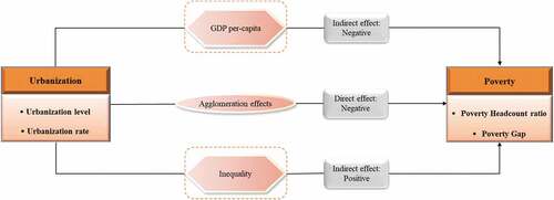The initial levels of per-capita GDP and inequality and the changes in per-capita GDP and inequality are used as the set of control variables (Dollar et al., 2016; Dollar & Kraay, 2002; Fosu, 2017; Kanbur, 2005). For the interaction terms, the level of urbanization is interacted each with per-capita GDP and Inequality to investigate the respective effects of per-capita GDP growth and changes in Inequality on the poverty reduction effect of urbanization. The interaction effects are computed and discussed in line with prior literature (Castells-Quintana & Wenban-Smith, 2020; Wang et al., 2022). Figure 1 presents the analytical framework of the study.

Figure 1. Analytical framework of the study.

The Cobb-Douglas functional specification of Equation 1(1) ${\mathrm{P}}_{\mathrm{i}\mathrm{t}}={\mathrm{A}\mathrm{U}}_{\mathrm{i}\mathrm{t}}^{\text{o}\left(1+\mathrm{l}\mathrm{n}\mathrm{U}\right)}{\mathrm{K}}_{\mathrm{i}\mathrm{t}}^{\mu }{\mathrm{R}}_{\mathrm{i}\mathrm{t}}^{\mathrm{\Omega }}$(1) is to make it easier to log-transform it to obtain the urbanization elasticity parameters for estimation. The log-linearization provides additional estimation benefits. First, it transforms the non-linear equation into a linear model to enable the parameters to be estimated using linear regression methods for easy interpretation. Second, the log-transformation reduces the skewness in the data which may be caused by outliers that may bias the estimated results. Third, it eliminates any possible existence of heteroscedasticity to make the error terms homoscedastic, uncorrelated and normally distributed.

Accordingly, the natural logarithm is taken on both sides of Equation 1(1) ${\mathrm{P}}_{\mathrm{i}\mathrm{t}}={\mathrm{A}\mathrm{U}}_{\mathrm{i}\mathrm{t}}^{\text{o}\left(1+\mathrm{l}\mathrm{n}\mathrm{U}\right)}{\mathrm{K}}_{\mathrm{i}\mathrm{t}}^{\mu }{\mathrm{R}}_{\mathrm{i}\mathrm{t}}^{\mathrm{\Omega }}$(1) and rewritten in a dynamic form to yield a first order autoregressive [AR (1)] model to be estimated as:

(2) ${\mathrm{p}}_{\mathrm{i}\mathrm{t}}=\mathrm{a}+\alpha {\mathrm{p}}_{\mathrm{i},\mathrm{t}-1}\hspace{0.17em}+\hspace{0.17em}{\beta }_1{\mathrm{u}}_{\mathrm{i}\mathrm{t}}+{\beta }_2{{\mathrm{u}}_{\mathrm{i}\mathrm{t}}}^2+\gamma {\mathrm{k}}_{\mathrm{i}\mathrm{t}}+\mathrm{\Omega }{\mathrm{r}}_{\mathrm{i}\mathrm{t}}+{\xi }_{\mathrm{i}\mathrm{t}}$(2)

where i = 1, …, N, t = 1, …, T and $\mathrm{p}=\mathrm{l}\mathrm{n}\mathrm{P},\mathrm{a}=\mathrm{l}\mathrm{n}\mathrm{A},\mathrm{u}=\mathrm{l}\mathrm{n}\mathrm{U},\mathrm{k}=\mathrm{l}\mathrm{n}\mathrm{K}\mathrm{a}\mathrm{n}\mathrm{d}\mathrm{r}=\mathrm{l}\mathrm{n}\mathrm{R}$. The parameters $\mathrm{a},$ α,$\hspace{0.17em}{\beta }_1,\hspace{0.17em}{\beta }_2,\hspace{0.17em}\gamma \hspace{0.17em}$ and $\mathrm{\Omega }$ are scalars with the subscript t denoting 5-year time interval. The squared term is included to capture any possible non-linear effects of urbanization on poverty.

The random disturbance term ${\xi }_{it\hspace{0.17em}}$ in the dynamic panel data (DPD) model of Equation 2(2) ${\mathrm{p}}_{\mathrm{i}\mathrm{t}}=\mathrm{a}+\alpha {\mathrm{p}}_{\mathrm{i},\mathrm{t}-1}\hspace{0.17em}+\hspace{0.17em}{\beta }_1{\mathrm{u}}_{\mathrm{i}\mathrm{t}}+{\beta }_2{{\mathrm{u}}_{\mathrm{i}\mathrm{t}}}^2+\gamma {\mathrm{k}}_{\mathrm{i}\mathrm{t}}+\mathrm{\Omega }{\mathrm{r}}_{\mathrm{i}\mathrm{t}}+{\xi }_{\mathrm{i}\mathrm{t}}$(2) is a one-way error component model of the form:

(3) ${\xi }_{it}={\upsilon }_i+{\epsilon }_{it}$(3)

where ${\upsilon }_i$ denotes the country-specific effects and ${\epsilon }_{it}$ is the usual stochastic error term. Equation 3(3) ${\xi }_{it}={\upsilon }_i+{\epsilon }_{it}$(3) is a random model, the error terms $\hspace{0.17em}{\upsilon }_i$ ∼IID (0, σ² ${\upsilon }_i$), ${\epsilon }_{it}$∼IID (0, σ² ${\epsilon }_{it})\hspace{0.17em}$ and are all independent such that E(${\upsilon }_i$) = 0, E (${\epsilon }_{it}$) = 0 and E (${\upsilon }_i\hspace{0.17em}{\epsilon }_{it}$) = 0. Also, the explanatory variables (${X_{\mathrm{i}\mathrm{t}}}^{\ast }$) in Equation 2(2) ${\mathrm{p}}_{\mathrm{i}\mathrm{t}}=\mathrm{a}+\alpha {\mathrm{p}}_{\mathrm{i},\mathrm{t}-1}\hspace{0.17em}+\hspace{0.17em}{\beta }_1{\mathrm{u}}_{\mathrm{i}\mathrm{t}}+{\beta }_2{{\mathrm{u}}_{\mathrm{i}\mathrm{t}}}^2+\gamma {\mathrm{k}}_{\mathrm{i}\mathrm{t}}+\mathrm{\Omega }{\mathrm{r}}_{\mathrm{i}\mathrm{t}}+{\xi }_{\mathrm{i}\mathrm{t}}$(2) are all orthogonal to the error terms ${\upsilon }_i$ and ${\epsilon }_{it}$ for all i and t such that E(${\upsilon }_i{X_{\mathrm{i}\mathrm{t}}}^{\ast }$) = E($\hspace{0.17em}{\epsilon }_{it}{X_{\mathrm{i}\mathrm{t}}}^{\ast }$) = E (${\xi }_{\mathrm{i}\mathrm{t}}{X_{\mathrm{i}\mathrm{t}}}^{\ast }$) = 0. Since both the dependent and the main independent variables in Equation 2(2) ${\mathrm{p}}_{\mathrm{i}\mathrm{t}}=\mathrm{a}+\alpha {\mathrm{p}}_{\mathrm{i},\mathrm{t}-1}\hspace{0.17em}+\hspace{0.17em}{\beta }_1{\mathrm{u}}_{\mathrm{i}\mathrm{t}}+{\beta }_2{{\mathrm{u}}_{\mathrm{i}\mathrm{t}}}^2+\gamma {\mathrm{k}}_{\mathrm{i}\mathrm{t}}+\mathrm{\Omega }{\mathrm{r}}_{\mathrm{i}\mathrm{t}}+{\xi }_{\mathrm{i}\mathrm{t}}$(2) are in natural logarithms, it implies that the coefficient of the main independent variables namely $\hspace{0.17em}{\beta }_1$ is the urbanization elasticity of poverty.

3.4. The case for generalized methods of moments

The application of the GMM methodology for this study is based on four principal reasons. First, the primary condition for the use of GMM exists since the number of countries (N = 29) is considerably higher than the number of time periods in each cross section (T = 7). Thus N >T. Second, the poverty indices are persistent. In particular, the correlation between the Poverty Headcount ratio (Poverty Gap) and its first lag is 0.8713 (0.8627) which is significant at 1% level. These coefficients are above the threshold level of 0.8000 required to establish the persistence of a variable (Asongu & Acha-Anyi, 2019; Tchamyou & Asongu, 2017). Third, the GMM preserves the cross-country variations in the panel data.

Fourth, there is a problem of endogeneity in Equation 2(2) ${\mathrm{p}}_{\mathrm{i}\mathrm{t}}=\mathrm{a}+\alpha {\mathrm{p}}_{\mathrm{i},\mathrm{t}-1}\hspace{0.17em}+\hspace{0.17em}{\beta }_1{\mathrm{u}}_{\mathrm{i}\mathrm{t}}+{\beta }_2{{\mathrm{u}}_{\mathrm{i}\mathrm{t}}}^2+\gamma {\mathrm{k}}_{\mathrm{i}\mathrm{t}}+\mathrm{\Omega }{\mathrm{r}}_{\mathrm{i}\mathrm{t}}+{\xi }_{\mathrm{i}\mathrm{t}}$(2) since ${\mathrm{p}}_{\mathrm{i}\mathrm{t}}$ as a function of ${\upsilon }_i$ implies that ${\mathrm{p}}_{\mathrm{i},\mathrm{t}-1}$ is also related to ${\upsilon }_i$ and therefore, using ${\mathrm{p}}_{\mathrm{i},\mathrm{t}-1}$ as a separate regressor will be correlated with the disturbance term $\hspace{0.17em}{\xi }_{\mathrm{i}\mathrm{t}}$. GMM addresses this endogeneity issue in several ways. It mitigates both the unmeasured and time-invariant individual country specific and unobserved heterogeneity effects (Asongu et al., 2020). It also accounts for simultaneity in the explanatory variables via the use of the lagged values of the dependent variable and the regressors as instruments in differences or both differences and levels (Bond & Windmeijer, 2002; Brülhart & Sbergami, 2009; Tchamyou et al., 2019). The GMM also uses the orthogonality conditions to obtain efficient and consistent estimates even when heteroskedasticity exists in an arbitrary form (Baum et al., 2003).

To illustrate the GMM procedure, consider Equation 2(2) ${\mathrm{p}}_{\mathrm{i}\mathrm{t}}=\mathrm{a}+\alpha {\mathrm{p}}_{\mathrm{i},\mathrm{t}-1}\hspace{0.17em}+\hspace{0.17em}{\beta }_1{\mathrm{u}}_{\mathrm{i}\mathrm{t}}+{\beta }_2{{\mathrm{u}}_{\mathrm{i}\mathrm{t}}}^2+\gamma {\mathrm{k}}_{\mathrm{i}\mathrm{t}}+\mathrm{\Omega }{\mathrm{r}}_{\mathrm{i}\mathrm{t}}+{\xi }_{\mathrm{i}\mathrm{t}}$(2) in level given in a general form as:

(4) ${{\mathrm{p}}_{\mathrm{i}\mathrm{t}}}^{\ast }=\alpha { }^{\mathrm{\prime }}{{\mathrm{p}}_{\mathrm{i},\mathrm{t}-1}}^{\ast }+\beta { }^{\mathrm{\prime }}{x_{\mathrm{i}\mathrm{t}}}^{\ast }+{\upsilon }_{\mathrm{i}}+{\epsilon }_{it}$(4)

where, ${{\mathrm{p}}_{\mathrm{i}\mathrm{t}}}^{\ast }$ represents the dependent variable and ${x_{\mathrm{i}\mathrm{t}}}^{\ast }$ the right-hand variables in Equation 2(2) ${\mathrm{p}}_{\mathrm{i}\mathrm{t}}=\mathrm{a}+\alpha {\mathrm{p}}_{\mathrm{i},\mathrm{t}-1}\hspace{0.17em}+\hspace{0.17em}{\beta }_1{\mathrm{u}}_{\mathrm{i}\mathrm{t}}+{\beta }_2{{\mathrm{u}}_{\mathrm{i}\mathrm{t}}}^2+\gamma {\mathrm{k}}_{\mathrm{i}\mathrm{t}}+\mathrm{\Omega }{\mathrm{r}}_{\mathrm{i}\mathrm{t}}+{\xi }_{\mathrm{i}\mathrm{t}}$(2) , with $a\mathrm{\prime }$ and $\beta { }^{\mathrm{\prime }}$ being parameters. The difference GMM (DIF-GMM) involves taking the first difference of Equation (5)(5) ${{\mathrm{p}}_{\mathrm{i}\mathrm{t}}}^{\ast }-{{\mathrm{p}}_{\mathrm{i},\mathrm{t}-1}}^{\ast }=\alpha { }^{\mathrm{\prime }}({{\mathrm{p}}_{\mathrm{i},\mathrm{t}-1}}^{\ast }-{{\mathrm{p}}_{\mathrm{i},\mathrm{t}-2}}^{\ast })+\beta { }^{\mathrm{\prime }}({x_{\mathrm{i}\mathrm{t}}}^{\ast }-{x_{\mathrm{i},\mathrm{t}-1}}^{\ast })+({\epsilon }_{\mathrm{i}\mathrm{t}}-{\epsilon }_{\mathrm{i},\mathrm{t}-1})$(5) as:

(5) ${{\mathrm{p}}_{\mathrm{i}\mathrm{t}}}^{\ast }-{{\mathrm{p}}_{\mathrm{i},\mathrm{t}-1}}^{\ast }=\alpha { }^{\mathrm{\prime }}({{\mathrm{p}}_{\mathrm{i},\mathrm{t}-1}}^{\ast }-{{\mathrm{p}}_{\mathrm{i},\mathrm{t}-2}}^{\ast })+\beta { }^{\mathrm{\prime }}({x_{\mathrm{i}\mathrm{t}}}^{\ast }-{x_{\mathrm{i},\mathrm{t}-1}}^{\ast })+({\epsilon }_{\mathrm{i}\mathrm{t}}-{\epsilon }_{\mathrm{i},\mathrm{t}-1})$(5)

Which can be rewritten in the form:

(6) $\mathrm{\Delta }{{\mathrm{p}}_{\mathrm{i}\mathrm{t}}}^{\ast }=\alpha { }^{\mathrm{\prime }}\mathrm{\Delta }{{\mathrm{p}}_{\mathrm{i},\mathrm{t}-1}}^{\ast }+\beta { }^{\mathrm{\prime }}\mathrm{\Delta }{x_{\mathrm{i}\mathrm{t}}}^{\ast }+\mathrm{\Delta }{\epsilon }_{\mathrm{i}\mathrm{t}}$(6)

where $\mathrm{\Delta }\hspace{0.17em}$ is the difference operator. The first differencing eliminates the country-specific effects term ${\upsilon }_{\mathrm{i}}$ which may result in incorrect model specification. Also, $\mathrm{\Delta }{{\mathrm{p}}_{\mathrm{i}\mathrm{t}}}^{\ast }$ is correlated with $\mathrm{\Delta }{\epsilon }_{it}$. The system GMM (SYS-GMM) is proposed to address the weak instrumentation problem of the DIF-GMM by combining instruments in first differences and levels (Bowsher, 2002; Judson & Owen, 1999; Roodman, 2009a). Also, the GMM procedure addresses the serial correlation and endogeneity issues through the use of sufficient lags of the dependent variable and the first differenced errors (Arellano & Bond, 1991; Arellano & Bover, 1995; Blundell & Bond, 1998).

3.5. Choosing between the difference and system GMM

In choosing between the DIF-GMM and SYS-GMM, the study follows the methodology outlined by Bond (2002). It involves estimating Equation 2 using the pooled OLS, Fixed Effects (FE) and DIF-GMM and comparing the respective values of $\alpha$. The OLS and the FE are considered, respectively, as an upper-bound estimate and lower-bound estimate. Since the a priori expectation is that $\alpha$ is positively correlated with ${\xi }_{\mathrm{i}\mathrm{t}}$, the OLS will bias its value upward whereas the FE will bias it downward so the estimated value of the true parameter should lie in or close to this range (Bond, 2002; Roodman, 2009b).

The results from the alternative estimations of Equation 2(2) ${\mathrm{p}}_{\mathrm{i}\mathrm{t}}=\mathrm{a}+\alpha {\mathrm{p}}_{\mathrm{i},\mathrm{t}-1}\hspace{0.17em}+\hspace{0.17em}{\beta }_1{\mathrm{u}}_{\mathrm{i}\mathrm{t}}+{\beta }_2{{\mathrm{u}}_{\mathrm{i}\mathrm{t}}}^2+\gamma {\mathrm{k}}_{\mathrm{i}\mathrm{t}}+\mathrm{\Omega }{\mathrm{r}}_{\mathrm{i}\mathrm{t}}+{\xi }_{\mathrm{i}\mathrm{t}}$(2) for the Poverty Headcount ratio and Poverty Gap as the respective dependent variables for the rates and levels of urbanization are presented in Table 2. From the Table, the coefficients of the respective lagged dependent variables from the DIF-GMM1 estimations are closer to that of the FE estimations, implying that the DIF-GMM estimator is biased downward and hence the SYS-GMM estimator is preferable in all cases.

Table 2. Alternative estimates for the lagged dependent variable ($\alpha )$ of Equation (2)(2) ${\mathrm{p}}_{\mathrm{i}\mathrm{t}}=\mathrm{a}+\alpha {\mathrm{p}}_{\mathrm{i},\mathrm{t}-1}\hspace{0.17em}+\hspace{0.17em}{\beta }_1{\mathrm{u}}_{\mathrm{i}\mathrm{t}}+{\beta }_2{{\mathrm{u}}_{\mathrm{i}\mathrm{t}}}^2+\gamma {\mathrm{k}}_{\mathrm{i}\mathrm{t}}+\mathrm{\Omega }{\mathrm{r}}_{\mathrm{i}\mathrm{t}}+{\xi }_{\mathrm{i}\mathrm{t}}$(2)

	Urbanization level and poverty		Urbanization rate and poverty
	Equation (2(2) ${\mathrm{p}}_{\mathrm{i}\mathrm{t}}=\mathrm{a}+\alpha {\mathrm{p}}_{\mathrm{i},\mathrm{t}-1}\hspace{0.17em}+\hspace{0.17em}{\beta }_1{\mathrm{u}}_{\mathrm{i}\mathrm{t}}+{\beta }_2{{\mathrm{u}}_{\mathrm{i}\mathrm{t}}}^2+\gamma {\mathrm{k}}_{\mathrm{i}\mathrm{t}}+\mathrm{\Omega }{\mathrm{r}}_{\mathrm{i}\mathrm{t}}+{\xi }_{\mathrm{i}\mathrm{t}}$(2) )		Equation (2)
Estimation	(2a)	(2b)	(2c)	(2d)
Dependent Variable	ln(Poverty Headcount)	ln(Poverty Gap)	ln(Poverty Headcount)	ln(Poverty Gap)
OLS	0.750(0.000)	0.763(0.000)	0.746(0.000)	0.702(0.000)
FE (within)	0.620(0.000)	0.572(0.000)	0.628(0.000)	0.471(0.000)
DIFF-GMM1	0.343(0.000)	0.240(0.000)	0.350(0.000)	0.141(0.017)
Bond (2002) Suggestion	SYS-GMM	SYS-GMM	SYS-GMM	SYS-GMM

Furthermore, in line with the convention in most applied work using GMM estimations, this study estimates and interprets the results of Equation (2)(2) ${\mathrm{p}}_{\mathrm{i}\mathrm{t}}=\mathrm{a}+\alpha {\mathrm{p}}_{\mathrm{i},\mathrm{t}-1}\hspace{0.17em}+\hspace{0.17em}{\beta }_1{\mathrm{u}}_{\mathrm{i}\mathrm{t}}+{\beta }_2{{\mathrm{u}}_{\mathrm{i}\mathrm{t}}}^2+\gamma {\mathrm{k}}_{\mathrm{i}\mathrm{t}}+\mathrm{\Omega }{\mathrm{r}}_{\mathrm{i}\mathrm{t}}+{\xi }_{\mathrm{i}\mathrm{t}}$(2) using the two-step system-GMM (SYS-GMM2). Several simulation studies have shown the efficiency gains from using SYS-GMM2 including controlling for heteroskedasticity and cross correlation (Bond & Windmeijer, 2002; Roodman, 2009a, 2009b; Windmeijer, 2005).

3.6. GMM specification tests

Following the convention in the literature, the study employs two main GMM standard specification tests. These are serial correlation tests, namely the first order [AR(1)] and the second order [AR(2)]; and the test on the validity of instruments (Arellano & Bond, 1991). Generally, using lagged variables as moment conditions can lead to bias due to the possibility of over-fitting the endogenous regressors (Baltagi, 2005). Consequently, the study follows (Bond, 2002; Roodman, 2009a, 2009b) and uses both the Sargan test and the Hansen test as complementary test statistics of full instrument validity as well as the structural specification of the model. Additionally, the collapsed approach of Roodman (2009a, 2009b) is adopted to account for cross-sectional dependence (Asongu & Acha-Anyi, 2019; Tchamyou et al., 2019) and to prevent instrument proliferation that weakens the Hansen J-test (Andersen & Sørensen, 1996; Bowsher, 2002).

3.7. GMM identification, simultaneity, and exclusive restrictions

Fundamental to the GMM strategy is the identification, simultaneity and exclusion restrictions. First, identification involves defining the three variable categories, namely the dependent variable, the endogenous explanatory variables and strictly exogenous variables (Asongu et al., 2020; Tchamyou et al., 2019). The outcome variables are the Poverty Headcount ratio and the Poverty Gap. The identified strictly exogenous variables are years whereas the explanatory variables, namely urbanization (rate and level) and the control variables are the endogenous variables (Asongu & Acha-Anyi, 2019; Tchamyou, 2019). Implicitly, the strictly exogenous variables are assumed to affect the outcome variable through the endogenous variables (Asongu et al., 2020).

Secondly, the issue of simultaneity such as the inclusion of both the urbanization term (${\mathrm{u}}_{\mathrm{i}\mathrm{t}}$) and the poverty term (${\mathrm{p}}_{\mathrm{i}\mathrm{t}}$) in Equation 2(2) ${\mathrm{p}}_{\mathrm{i}\mathrm{t}}=\mathrm{a}+\alpha {\mathrm{p}}_{\mathrm{i},\mathrm{t}-1}\hspace{0.17em}+\hspace{0.17em}{\beta }_1{\mathrm{u}}_{\mathrm{i}\mathrm{t}}+{\beta }_2{{\mathrm{u}}_{\mathrm{i}\mathrm{t}}}^2+\gamma {\mathrm{k}}_{\mathrm{i}\mathrm{t}}+\mathrm{\Omega }{\mathrm{r}}_{\mathrm{i}\mathrm{t}}+{\xi }_{\mathrm{i}\mathrm{t}}$(2) is addressed through the instrumentation process of the SYS-GMM (Arellano & Bover, 1995; Bond & Windmeijer, 2002; Roodman, 2009b). Third, the exclusive restrictions involve checking the validity of a subset of instruments (Roodman, 2009a, 2009b). Within the GMM strategy, the Difference in Hansen Test is applied and the validity of the exclusion restrictions is confirmed when the null hypothesis in relation to the instrumental variable is not rejected (Asongu & Acha-Anyi, 2019; Asongu et al., 2020).

4. Results and discussions

4.1. Correlations among key variables

The partial correlation matrix among the key variables is reported in Table 3. The poverty reduction effect of urbanization as indicated by the negative correlation coefficients between urbanization level and the Poverty Headcount ratio (Poverty Gap) is −0.543 (−0.431) and significant at 1% level. Similarly, the correlation between GDP per-capita and the Poverty Headcount ratio (Poverty Gap) is −0.603 (−0.495) and significant at 1% level. The correlation coefficients between the Gini indices and the poverty indices are all positive, albeit only that between the Gini Index and the Poverty Gap is significant at 1% level.

Table 3. Correlation matrix of key variables

Variables	(1)	(2)	(3)	(4)	(5)	(6)	(7)	(8)
(1) Poverty Headcount ratio	1.000
(2) Poverty Gap	0.936***	1.000
(3) Urbanization rate	0.137*	0.084	1.000
(4) Urbanization level	−0.543***	−0.431***	−0.377***	1.000
(5) GDP per-capita growth	−0.133*	−0.173**	0.075	−0.110	1.000
(6) Gini index growth	0.088	0.123	0.220***	−0.030	−0.082	1.000
(7) GDP per-capita	−0.603***	−0.495***	−0.146**	0.730***	−0.026	0.031	1.000
(8) Gini index	0.024	0.182***	−0.037	0.148**	−0.024	0.319***	0.307***	1.000

Note: */** /*** indicate statistically significant levels at, respectively, 10%/5%/1%.

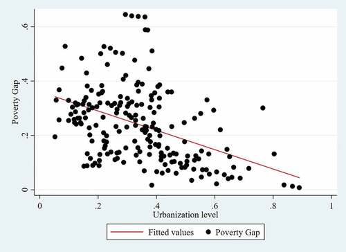
Furthermore, the scatterplot in Figures 2 and 3 show strong negative correlations between the level of urbanization and the poverty indices in SSA. This attests to the poverty reduction effect of urbanization. However, due to the absence of control mechanisms and diagnostic tests not much inference is made from these graphical results.

Figure 2. Scatterplot of the relationship between urbanization level and the poverty headcount: 1985–2019.

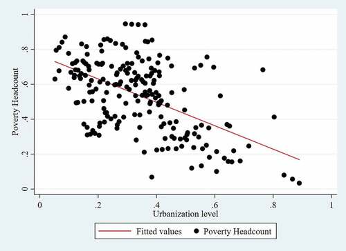
Figure 3. Scatterplot of the relationship between urbanization level and the poverty gap: 1985–2019.

4.2. Effects of urbanization on poverty

The results for the SYS-GMM2 estimations of Equation 2(2) ${\mathrm{p}}_{\mathrm{i}\mathrm{t}}=\mathrm{a}+\alpha {\mathrm{p}}_{\mathrm{i},\mathrm{t}-1}\hspace{0.17em}+\hspace{0.17em}{\beta }_1{\mathrm{u}}_{\mathrm{i}\mathrm{t}}+{\beta }_2{{\mathrm{u}}_{\mathrm{i}\mathrm{t}}}^2+\gamma {\mathrm{k}}_{\mathrm{i}\mathrm{t}}+\mathrm{\Omega }{\mathrm{r}}_{\mathrm{i}\mathrm{t}}+{\xi }_{\mathrm{i}\mathrm{t}}$(2) are presented in Tables 4, 5 and Table 6. All estimations were conducted at 95% confidence interval and the maximum lag length of the variables and instruments are restricted to three (3) which according to the simulation studies of Bowsher (2002) maximizes the power of the Sargan test.

Table 4. Regression results for urbanization and poverty headcount ratio

Estimation	Urbanization Rate and Poverty Headcount ratio		Urbanization level and poverty headcount ratio
Dependent Variable: ln(Poverty Headcount)	Two-step SYS-GMM (1)	Two-step SYS-GMM (2)	Two-step SYS-GMM (1)	Two-step SYS-GMM (2)
Lagged [ln(Poverty Headcount)]	0.49(0.65)***	0.97(0.25)***	0.64(0.12)***	1.74(0.92)*
ln(Urbanization rate)	−0.04(0.02)**	−0.07(0.03)***
ln(Urbanization level)			−0.22(0.08)***	−0.60(0.27)**
ln(per-capita GDP growth)	−0.42(0.29)		−0.33(0.39)
Squared (per capita GDP growth)	−7.00(3.46)*	−13.79(7.56)*	−11.52(5.00)**	−31.55(16.15)*
ln(Inequality growth)	0.52(0.11)***	1.02(0.27)***	0.27(0.17)
Squared (Inequality growth)	0.2(0.31)		−0.98(0.33)***	−2.69(1.26)**
ln(Initial Inequality)	0.16(0.09)*	0.32(0.16)**	−0.01(0.11)
ln(Initial per-capita GDP)	−0.12(0.04)***	−0.23(0.07)***	−0.08(0.05)
Initial Urbanization level	−0.11(0.04)**	−0.22(0.08)***
Urbanization level*Inequality Level	1.04(0.44)**	2.04(0.88)**	1.53(0.66)**	4.2(1.91)**
Urbanization level*per-capita GDP	−0.0001(0.00002)***	−0.0002(0.00003)***	−0.0001(0.00002)***	−0.0002(0.0001)***
Time effects	−0.07(0.01)***	−0.13(0.02)***	−0.04(0.02)**	−0.11(0.04)***
Constant	0.55(0.31)*		0.11(39)
Countries	29		29
T	7		7
Observations	174		145
No. of Instruments	27		23
F-test	359.13 (0.00)		210.10 (0.00)
AR(1)	−2.12 (0.34)		−1.86 (0.06)
AR(2)	−0.91 (0.36)		−0.41 (0.68)
Sargan	21.07 (0.10)		14.53 (0.21)
Hansen	14.25 (0.43)		11.10 (0.44)
Difference in Hansen Test
(a) Instruments for levels
H excluding group	10.08 (0.44)		7.54 (0.48)
Dif(null H = exogenous)	4.17 (0.38)		3.56 (0.31)
(b) Instumental variables
H excluding group	1.51 (0.82)		0.47 (0.79)
Dif(null H = exogenous)	12.74 (0.24)		10.64 (0.30)

Notes: */** /*** indicate significance levels at, respectively, 10%/5%/1%. The standard errors for the estimated parameters are in parenthesis. For the F, AR(1), AR(2), Sargan, Hansen and Difference in Hansen tests, the p-values are in parenthesis. The panel data cover the period from 1985–2019 and the variables are calculated over 5-year intervals. Also, (1) = short-run estimates; (2) = long-run estimates.

Table 5. Regression results for urbanization and poverty gap

Estimation	Urbanization Rate and Poverty Gap		Urbanization Level and Poverty Gap
Dependent Variable: ln(Poverty Gap)	Two-step SYS-GMM (1)	Two-step SYS-GMM (2)	Two-step SYS-GMM (1)	Two-step SYS-GMM (2)
Lagged [ln(Poverty Gap)]	0.44(0.11)***	0.80(0.34)**	0.52(0.07)***	1.09(0.29)***
ln(Urbanization rate)	-0.05(0.03)**	-0.09(0.04)**
ln(Urbanization level)			-0.32(0.10)***	-0.68(0.18)***
ln(per-capita GDP growth)	-1.48(0.44)***	-2.67(0.81)***	-1.13(0.33)***	-2.36(0.74)***
Squared (per capita GDP growth)	-13.53(3.42)***	-24.36(8.55)***	-10.20(3.33)***	-21.29(7.28)***
ln(Inequality growth)	1.18(0.16)***	2.12(0.55)***	0.57(0.21)**	1.20(0.52)**
Squared (Inequality growth)	0.90(0.43)**	1.62(0.60)***	0.15(0.43)
Initial Inequality	0.17(0.18)		0.06(0.10)
Initial per-capita GDP	-0.17(0.07)**	-0.30(0.11)***	-0.20(0.04)***	-0.41(0.05)***
ln(Initial Urbanization level)	-0.29(0.10)***	-0.52(0.13)***
Urbanization level*Inequality Level	3.42(0.93)***	6.15(1.20)***	3.21(0.73)***	6.69(0.96)***
Urbanization level*per-capita GDP	-0.0002(0.00003)***	-0.0003(0.00004)***	-0.0001(0.00002)***	-0.0003(0.00002)***
Time effects	-0.12(0.01)***	-0.21(0.04)***	-0.08(0.02)***	-0.16(0.03)***
Constant	0.03(0.49)		0.33(0.16)*
Countries	29		29
T	6		6
Observations	174		174
No. of Instruments	29		29
F-test	807.38 (0.00)		774.45 (0.00)
AR(1)	-2.3 (0.02)		-2.38 (0.02)
AR(2)	-1.21 (0.23)		-1.37 (0.17)
Sargan	13.86 (0.61)		16.82 (0.45)
Hansen	21.01 (0.18)		21.49 (0.21)
Difference in Hansen Test
(a) Instruments for levels
H excluding group	15.73 (0.20)		13.92 (0.38)
Dif(null H=exogenous)	5.28 (0.26)		7.57 (0.11)
(b) Instumental variables
H excluding group	8.82 (0.18)		12.29 (0.14)
Dif(null H=exogenous)	12.20 (0.27)		9.20 (0.42)

Notes: */** /*** indicate significance levels at, respectively, 10%/5%/1%. The standard errors for the estimated parameters are in parenthesis. For the F, AR(1), AR(2), Sargan, Hansen and Difference in Hansen tests, the p-values are in parenthesis. The panel data cover the period from 1985–2019 and the variables are calculated over 5-year intervals. Also, (1) = short-run estimates; (2) = long-run estimates.

Table 6. Comparing the growth rates and levels of urbanization elasticities of poverty

	Growth rates of Urbanization and Poverty Indices			Levels of Urbanization and Poverty Indices
Estimated Equation	2	2		2	2
Table No.	Table 4	Table 5		Table 4	Table 5
Dependent Variable	ln(Poverty Headcount)	ln(Poverty Gap)	Dominant effect	ln(Poverty Headcount)	ln(Poverty Gap)	Dominant effect
Main Explanatory Variable	Lagged [ln(Urbanization rate)]	Lagged [ln(Urbanization rate)]		Lagged [ln(Urbanization level)]	Lagged [ln(Urbanization level)]
Short-run elasticity	-0.04	-0.05	Poverty Gap	-0.22	-0.32	Poverty Gap
	(0.02)**	(0.03)**		(0.08)***	(0.10)***
Long-run elasticity	-0.07	-0.09	Poverty Gap	-0.60	-0.68	Poverty Gap
	(0.03)***	(0.04)**		(0.27)**	(0.18)***

Notes: * / ** /*** indicate significance levels at respectively 10% / 5% / 1%. The standard errors for the estimated parameters are in parenthesis. The panel data cover the period from 1985-2019 and the variables are calculated over 5-year intervals.

Four criteria are used to evaluate the validity of each estimation (Asongu et al., 2020; Tchamyou et al., 2019). First is autocorrelation test. The AR (1) has the preferred negative sign and most importantly, the AR (2) is not significant in all estimations. This implies that the lag terms of the respective dependent variables used as instruments are exogenous and therefore valid instruments. It also confirms the appropriateness of the DPD models used for this study. Second is the test of full instrument validity. The p-values associated with the Sargan and Hansen tests for over-identification restrictions are all not significant. These confirm the validity of the full instruments used in each estimation. Particularly, the p-values for the J-statistics are within the generally acceptable range of 0.10–0.60 with that for the Poverty Gap being within the “Goldilocks range” of 0.10–0.25 (Roodman, 2009a). Third is the test of validity of instrument subset. The p-values for the Difference in Hansen Test are all not significant and confirm the exogeneity of the subsets of the instruments used. Fourth, the overall significance of each regression as indicated by the F-test statistic is significant at 1% level. The results from these standard diagnostic tests confirm the validity of the structural specifications and moment conditions used in estimating Equation (2)(2) ${\mathrm{p}}_{\mathrm{i}\mathrm{t}}=\mathrm{a}+\alpha {\mathrm{p}}_{\mathrm{i},\mathrm{t}-1}\hspace{0.17em}+\hspace{0.17em}{\beta }_1{\mathrm{u}}_{\mathrm{i}\mathrm{t}}+{\beta }_2{{\mathrm{u}}_{\mathrm{i}\mathrm{t}}}^2+\gamma {\mathrm{k}}_{\mathrm{i}\mathrm{t}}+\mathrm{\Omega }{\mathrm{r}}_{\mathrm{i}\mathrm{t}}+{\xi }_{\mathrm{i}\mathrm{t}}$(2) .

The estimated results from Tables 4 and 5 indicate the poverty reduction effect of urbanization in SSA. One, as indicated by the urbanization elasticities of poverty, the poverty reduction effect of urbanization is stronger in both magnitude and significance for the level of urbanization as compared to the rate of urbanization for the same poverty index. For example, for P₁ in Table 5, the respective estimated short-run and long-run urbanization level (rate) elasticities are −0.32 (−0.05) and −0.68 (−0.09) at corresponding 1% (5%) and 1% (5%) significant levels.⁴

Two, the poverty reduction effect of urbanization is stronger in the long-run as compared to the short-run for the same poverty index. For instance, for P₀ in Table 4 the long-run (short-run) magnitudes of the urbanization elasticity variables ln(Urbanization level) and ln(Urbanization rate) are, respectively, -0.60 (-0.22) and -0.07 (-0.04). A similar observation pertains to P₁ in Table 5. These elasticities imply that the poverty reduction effect of urbanization amplifies with time.

Three, in general, both the growth rate and initial level of per-capita GDP have significant poverty reduction effects. Particularly, from Table 5, the coefficients of the variables ln(per-capita GDP growth) and ln(Initial per-capita GDP) are negative and significant in both the short-run and long-run for P₁. These results are in line with the literature and specifically support the findings of (Bourguignon, 2003; Dollar et al., 2016; Dollar & Kraay, 2002; Fosu, 2009, 2017b) that high level of per-capita GDP and/or the growth rate of per-capita GDP is a boon to poverty reduction. More so, the general significance of the variable Squared(per-capita GDP growth) confirm the existence of a non-linear relationship between GDP per-capita and poverty. Further, the (absolute) magnitude of the growth elasticity of poverty ln(per-capita GDP growth) increases with time. For P₁ in Table 5, it increases from −1.48 (−1.13) in the short-run to −2.67 (−2.36) in the long-run for the urbanization rate (level).

Four, the results generally confirm the deleterious effect of income inequality on poverty. Particularly, the variable ln(Inequality growth) is significant throughout for P₁ in Table 5. However, the results for the initial level of inequality, although with the right positive coefficients, are only significant for P₀ in the long-run. On the whole, these results support the findings of Fosu (2009, 2017) and Kalwij and Verschoor (2007) that initial and/or growing inequality hurt poverty reduction efforts and converse to the findings of Dollar and Kraay (2002) and Dollar et al. (2016) that growth in income of the poor are uncorrelated with both the initial and growth in income distribution. Furthermore, the variable Squared (Inequality growth) being generally significant for both P₀ and P₁ in Tables 4 and 5 confirm the non-linear relationship between inequality and poverty.

Five, the respective roles of GDP per-capita and Inequality levels in moderating the effect of urbanization on poverty are as expected. The significance of respective positive and negative coefficients of the interaction effects variables, namely (Urbanization level*per-capita GDP) and (Urbanization level*Inequality Level) in both Tables 4 and 5 show that the poverty reduction effect of urbanization is amplified by the level of GDP per-capita and attenuated by the level of Inequality. The former results confirm the synergistic complementary relationship between the spatial agglomeration of economic activities and economic growth.

Six, Time effects are significant and increase in (absolute) magnitude for both poverty indices, a result that corroborates with the generally observable increasing poverty reduction effects of the significant variables in the long-run.

4.3. Comparing urbanization elasticities for the poverty indices

Table 6 presents a summary of the urbanization elasticities of poverty estimated from Equation 2.(2) ${\mathrm{p}}_{\mathrm{i}\mathrm{t}}=\mathrm{a}+\alpha {\mathrm{p}}_{\mathrm{i},\mathrm{t}-1}\hspace{0.17em}+\hspace{0.17em}{\beta }_1{\mathrm{u}}_{\mathrm{i}\mathrm{t}}+{\beta }_2{{\mathrm{u}}_{\mathrm{i}\mathrm{t}}}^2+\gamma {\mathrm{k}}_{\mathrm{i}\mathrm{t}}+\mathrm{\Omega }{\mathrm{r}}_{\mathrm{i}\mathrm{t}}+{\xi }_{\mathrm{i}\mathrm{t}}$(2) Estimations at growth rates indicate that a 1 percentage point increase in urbanization rate induces 0.04 (0.05) and 0.07 (0.09) percentage points decrease in the Poverty Headcount (Poverty Gap) in the short-run and the long-run, respectively. Similarly, estimation at levels indicate that a 1 percent increase in urbanization level induces 0.22 (0.32) and 0.60 (0.68) percent decrease in the Poverty Headcount (Poverty Gap) in the short-run and the long-run, respectively. Clearly, urbanization has a stronger effect in reducing the depth of poverty (P₁) relative to the incidence of poverty (P₀) in both the short-run and the long-run. Furthermore, the poverty reduction effect of urbanization at both growth rates and levels of urbanization are far more pronounced in the long-run relative to the short-run.

5. Summary and conclusions

The study investigated the poverty reduction effect of urbanization for a panel of 29 urbanizing countries in SSA from 1985 to 2019. The study employed the SYS-GMM2 to estimate the growth rates and levels of urbanization elasticities of poverty. The results show that urbanization within the selected SSA countries has a significant effect in reducing both the incidence of poverty (Poverty Headcount ratio) and depth of poverty (Poverty Gap) with the latter effect being consistently stronger than the former at both growth rates and levels in the short-run and long-run. Overall, the findings of this study reappraise the literature on the urbanization of poverty in SSA as well as provide a nuanced understanding of the effect of urbanization on the different class of poverty measures.

The findings of this study have several policy implications. First, due to its potential for poverty reduction, policy makers in SSA should fully embrace urbanization rather than adopt partial exclusionary measures to prevent it. Second, the full benefits of the urbanization process cannot be reaped automatically. This calls for long-term urban planning and substantial investment in the provision of urban public infrastructure and services such as roads, water, health, education, telecommunication, and others that are mostly lacking in the newly emerging and contiguous urban areas in SSA. Third, promoting (sustainable) urbanization must be made part and parcel of the process of nurturing economic growth and eradicating poverty in SSA. Four, to successfully manage the urbanization and its economic consequences in SSA, there is the need for continuous policy coordination across national and sub-regional borders in SSA. Five, promoting sustainable urbanization in SSA requires the provision of legal and effective enforcement of private property rights over land and buildings that constitute the urban built environment.

An obvious weakness of this study is its limited scope. For instance, the stylized facts of the spatial distribution of poverty worldwide show a declining incidence from rural areas to smaller towns and cities to metropolitan areas, however, urban poverty in many SSA countries is disproportionately concentrated in the largest cities (World Bank, 2011; World Bank & IMF, 2013). This phenomenon which was not examined in this study presents avenue for future research.

Disclosure statement

No potential conflict of interest was reported by the authors.

Additional information

Funding

The authors received no direct funding for this research.

Notes

1. The other five (5) regions are and Central Asia; East Asia and Pacific; Latin America and the Caribbean; Middle East and North Africa; and South Asia.

2. The use of the SYS-GMM addresses the issues of endogeneity, autocorrelation, and heteroscedasticity, thereby generating unbiased, consistent, and efficient results.

3. These are: Botswana, Burkina Faso, Burundi, Cameroon, Central African Republic, Chad, Democratic Republic of Congo, Côte d’Ivoire, Ethiopia, Gabon, Gambia, Ghana, Guinea, Guinea Bissau, Kenya, Lesotho, Madagascar, Malawi, Mali, Mozambique, Nigeria, Republic of Congo, Rwanda, Senegal, Sierra Leone, South Africa, Tanzania, Togo, Uganda.

4. Including the squared terms of the urbanization variables resulted in collinearity issues and were dropped in the estimations.

Appendix

Table A. Data Sources and Definitions

Table

Variables	Definitions/Measurements	Expected sign	Sources
Dependent Variables
Poverty Headcount (P0)	Percentage of population with income/consumption below the poverty line of $1.90 a day (2011 PPPs)		WDI
Poverty Gap (P1)	Mean shortfall in income/consumption from the poverty line $1.90 a day (2011 PPPs)		WDI
Urbanization variables
Urbanization rate	Average annual growth rate of urban population	Negative	WUP
Urbanization level	Percentage of total population living in areas described as cities by national statistics	Negative	WUP
Control variables
GDP per-capita	expenditure-side real GDP per-capita at chained PPPs (in million 2011 USD)	Negative	PWT
GDP growth rate	Annual percentage growth of real GDP per-capita (constant 2011 national prices)	Negative	Calculated from PWT data
Gini index	A measure of income distribution among individuals or households within an economy	Positive	WDI
Gini index growth	Changes in the measure of income distribution among individuals or households within an economy	Positive	Calculated from WDI data

PWT, Penn World Tables; WDI, World Development Indicators; WUP, World Urbanization Prospects

References

- Andersen, T. G., & Sørensen, B. E. (1996). GMM estimation of a stochastic volatility model: A Monte Carlo study. Journal of Business and Economic Statistics, 141, 328–20. https://www.tandfonline.com/doi/abs/10.1080/07350015.1996.10524660
- Annez, P. C., & Buckley, R. M. (2009). Urbanization and growth: Setting the context. In M. Spence, P. C. Annez, & R. M. Buckley (Eds.), Urbanization and growth. Commission on growth and development (pp. 1–45). World Bank.
- Arellano, M., & Bond, S. (1991). Some tests of specification for panel data: Monte Carlo evidence and an application to employment equations. The Review of Economic Studies, 58(2), 277–297. https://doi.org/10.2307/2297968
- Arellano, M., & Bover, O. (1995). Another look at the instrumental variable estimation of error-components models. Journal of Econometrics, 68(1), 29–51. https://doi.org/10.1016/0304-4076(94)01642-D
- Asongu, S. A., & Acha-Anyi, P. N. (2019). The murder epidemic: A global comparative study. International Criminal Justice Review, 29(2), 105–120. https://doi.org/10.1177/1057567718759584
- Asongu, S. A., Nnanna, J., & Acha-Anyi, P. N. (2020). On the simultaneous openness hypothesis: FDI, trade and TFP dynamics in Sub-Saharan Africa. Journal of Economic Structures, 9(1), 1–27. https://doi.org/10.1186/s40008-020-0189-4
- Baltagi, B. H. (2005). Econometric analysis of panel data (3rd edition ed.). John Wiley & Sons Ltd.
- Baum, C. F., Schaffer, M. E., & S, S. (2003). Instrumental variables and GMM: Estimation and testing. Stata Journal, 3(1), 1–31. https://doi.org/10.1177/1536867X0300300101
- Blundell, R., & Bond, S. (1998). Initial conditions and moment restrictions in dynamic panel data models. Journal of Econometrics, 87(1), 115–143. https://doi.org/10.1016/S0304-4076(98)00009-8
- Bond, S. (2002). Dynamic panel data models: A guide to micro data methods and practice. Centre for Microdata Methods and Practice Working Paper, No. CWP09/02, London. https://doi.org/10.1920/wp.cem.2002.0902
- Bond, S., & Windmeijer, F. (2002). Finite sample inference for GMM estimators in linear panel data models. Cenmap Working Paper Series No. CWP04/02. Institute of Fiscal Studies, London.
- Bourguignon, F. (2003). The growth elasticity of poverty reduction: Explaining heterogeneity across countries and time periods in:Inequality and growth: Theory and policy implications. MIT Press. In.
- Bowsher, C. G. (2002). On testing overidentifying restrictions in dynamic panel data models. Economics Letters, 77(2), 211–220. https://doi.org/10.1016/S0165-1765(02)00130-1
- Broto, V. C., Maria de Fátima, S., & Guibrunet, L. (2020). Energy profiles among urban elite households in Mozambique: Explaining the persistence of charcoal in urban areas. Energy Research & Social Science, 65, 101478. https://doi.org/10.1016/j.erss.2020.101478
- Brülhart, M., & Sbergami, F. (2009). Agglomeration and growth: Cross-country evidence. Journal of Urban Economics, 65(1), 48–63. https://doi.org/10.1016/j.jue.2008.08.003
- Cali, M., & Menon, C. (2013). Does urbanisation affect rural poverty? Evidence from Indian districts. The World Bank Economic Review, 27(2), 171–201. https://doi.org/10.1093/wber/lhs019
- Castells-Quintana, D. (2017). Malthus living in a slum: Urban concentration, infrastructure and economic growth. Journal of Urban Economics, 98, 158–173. https://doi.org/10.1016/j.jue.2016.02.003
- Castells-Quintana, D., & Wenban-Smith, H. (2020). Population dynamics, urbanisation without growth, and the rise of megacities. The Journal of Development Studies, 56(9), 1663–1682. https://doi.org/10.1080/00220388.2019.1702160
- Chauvin, J. P., Glaeser, E., Ma, Y., & Tobio, K. (2017). What is different about urbanization in rich and poor countries? Cities in Brazil, China, India and the United States. Journal of Urban Economics, 98, 17–49. https://doi.org/10.1016/j.jue.2016.05.003
- Christiaensen, L., Chuhan-Pole, P., & Sanoh, A. (2013). Africa’s growth, poverty and inequality nexus - fostering shared prosperity. World Bank Draft Paper.
- Christiaensen, L., & Weerdt, J. D. (2017). Urbanisation, growth and poverty reduction:The role of secondary towns. Final Report. International Growth Center.
- Collier, P. (2006). Africa: Geography and growth. Department of Economics. Centre for the Study of African Economies, Oxford University.
- Collier, P. (2017). African urbanization: An analytic policy guide. Oxford Review of Economic Policy, 33(3), 405–437. https://doi.org/10.1093/oxrep/grx031
- Collier, P., & Venables, A. J. (2017). Urbanization in developing economies: The assessment. Oxford Review of Economic Policy, 33(3), 355–372. https://doi.org/10.1093/oxrep/grx035
- da Mata, D., Deichmann, U., Henderson, V., Lall, S. V., & Wang, H. G. (2015). Determinants of city growth in Brazil. Journal of Urban Economics, 62(2), 252–272. https://doi.org/10.1016/j.jue.2006.08.010
- Datt, G., & Ravallion, M. (2009). Has India’s economic growth become more pro-poor in the wake of economic reforms? World Bank Policy Research Working Paper Series No, 5103. https://doi.org/10.1093/wber/lhr002
- Deichmann, U., Shilpi, F., & Vakis, R. (2009). Urban proximity, agricultural potential and rural non-farm employment: Evidence from Bangladesh. World Development, 37(3), 645–660. https://doi.org/10.1016/j.worlddev.2008.08.008
- Dollar, D., Kleineberg, T., & Kraay, A. (2016). Growth still is good for the poor. European Economic Review, 81, 68–85. https://doi.org/10.1016/j.euroecorev.2015.05.008
- Dollar, D., & Kraay, A. (2002). Growth is good for the poor. Journal of Economic Growth, 7(3), 195–225. https://doi.org/10.1023/A:1020139631000
- Emran, M. S., & Shilpi, F. (2012). The extent of the market and stages of agricultural specialization. Canadian Journal of Economics, 45(3), 1125–1153. https://doi.org/10.1111/j.1540-5982.2012.01729.x
- Fafchamps, M., & Shilpi, F. (2005). Cities and specialisation: Evidence from South Asia. The Economic Journal Royal Economic Society, 115(503), 477–504. https://doi.org/10.1111/j.1468-0297.2005.00997.x
- Fay, M., & Opal, C. (2000). Urbanization without growth: A not-so-uncommon phenomenon. The World Bank Policy Research Working Paper Series 2412. https://elibrary.worldbank.org/doi/abs/10.1596/1813-9450-2412
- Ferre, C., Ferreira, F. G. H., & Lanjouw, P. (2012). Is there a metropolitan bias? The relationship between poverty and city size in a selection of developing countries. World Bank Economic Review, 26(5508), 1–32. https://doi.org/10.1093/wber/lhs007
- Foster, J., Greer, J., & Thorbecke, E. (1984). A class of decomposable poverty measures. Econometrica, 52(3), 761–766. https://doi.org/10.2307/1913475
- Foster, A., & Rosenzweig, M. (2004). Agricultural development, industrialization and rural inequality. Brown University.
- Fosu, A. K. (2009). Inequality and the impact of growth on poverty: Comparative evidence for Sub-Saharan Africa. The Journal of Development Studies, 45(5), 726–745. https://doi.org/10.1080/00220380802663633
- Fosu, A. K. (2017). Growth, inequality and poverty reduction in developing countries: Recent global evidence. Research in Economics, 71(2), 306–336. https://doi.org/10.1016/j.rie.2016.05.005
- Fosu, A. K. (2017b). Growth, inequality and poverty reduction in developing countries: Recent global evidence. Research in Economics, 71(2), 306–336. https://doi.org/10.1016/j.rie.2016.05.005
- Fujita, M., Thisse, J.-F., Dewatripont, M., Hansen, L. P., & Turnovsky, S. J. (2003). Agglomeration and market interaction. Advances in Economics and Econometrics, 302–338. https://doi.org/10.1006/jjie.1996.0021
- Glaeser, E. L. (2013). A world of cities: The causes and consequences of urbanization in poorer countries. Journal of the European Economic Association, 12(5), 1154–1199 https://doi.org/10.1111/jeea.12100
- Glaeser, E., & Henderson, J. V. (2017). Urban economics for the developing World: An introduction. Journal of Urban Economics, 98, 1–5. https://doi.org/10.1016/j.jue.2017.01.003
- Gollin, D. (2018). Structural transformation without industrialization. Pathways for prosperity commission. Background Paper Series No. 2.
- Gollin, D., Hansen, C. W., & Wingender, A. (2021). Two blades of grass: The impact of the green revolution. Journal of Political Economy, 129(8), 2344–2384. https://www.journals.uchicago.edu/doi/full/10.1086/714444
- Gollin, D., Jedwab, R., & Vollrath, D. (2016). Urbanization with and without industrialization. Journal of Economic Growth, 21(1), 35–70. https://doi.org/10.1007/s10887-015-9121-4
- Ha, N. M., Dang Le, N., & Trung-Kien, P. (2021). The impact of urbanization on poverty reduction: An evidence from Vietnam. Cogent Economics & Finance, 9(1), 1918838. https://doi.org/10.1080/23322039.2021.1918838
- Henderson, J. V. (2000). The effects of urban concentration on economic growth. NBER Working Paper No. 7503. https://www.nber.org/papers/w7503.10.3386/w7503
- Henderson, J. V. (2003a). The urbanization process and economic growth: The so-what question. Journal of Economic Growth, 8(1), 47–71. https://doi.org/10.1023/A:1022860800744
- Henderson, J. V. (2003b). Marshall’s scale economies. Journal of Urban Economics, 53(1), 1–28. https://doi.org/10.1016/s0094-1190(02)00505-3
- Henderson, J. V., & Kriticos, S. (2017). The development of the African system of cities. Annual Review of Economics, 10, 1941–1383. http://eprints.lse.ac.uk/86349/
- Judson, R. A., & Owen, A. (1999). Estimating dynamic panel data models: A guide for macroeconomists. Economics Letters, 65(1), 9–15. https://doi.org/10.1016/S0165-1765(99)00130-5
- Kalwij, A., & Verschoor, A. (2007). Not by growth alone: The role of the distribution of income in regional diversity in poverty reduction. European Economic Review, 51(4), 805–829. https://doi.org/10.1016/j.euroecorev.2006.06.003
- Kanbur, R. (2005). Growth, inequality and poverty: Some hard questions. Journal of International Affairs, 58(2), 223–232. https://www.jstor.org/stable/24358274#metadata_info_tab_contents
- Lanjouw, P., & Marra, M. R. (2018). Urban poverty across the spectrum of Vietnam’s towns and cities. World Development, 110, 295–306. https://doi.org/10.1016/j.worlddev.2018.06.011
- Liddle, B. (2017). Urbanization and Inequality/Poverty. Urban Science, 1(4), 35. https://doi.org/10.3390/urbansci1040035
- Mahumane, G., & Mulder, P. (2022). Urbanization of energy poverty? The case of Mozambique. Renewable and Sustainable Energy Reviews, 159, 112089. https://doi.org/10.1016/j.rser.2022.112089
- McGranahan, G. (2017). Cities, urbanization and poverty reduction. Briefing Paper. SDC-IDS Collaboration on Poverty, Politics and Participatory Methodologies.
- McGranahan, G., & Satterthwaite, D. (2014). Urbanisation concepts and trends. International Institute for Environment and Development Working Paper: London.
- Nguyen, C. V. (2014). Does urbanization help poverty reduction in rural areas? Evidence from a developing country. IPAG Working Paper Series No. 178.
- Nguyen, H. M., & Nguyen, L. D. (2018). The relationship between urbanization and economic growth. International Journal of Social Economics, 45(2), 316–339. https://doi.org/10.1108/ijse-12-2016-0358
- Ravallion, M., Chen, S., & Sangraula, P. (2007). New evidence on the urbanization of global poverty. Population and development review, 33(4), 667–701. https://doi.org/10.1111/j.1728-4457.2007.00193.x
- Roodman, D. M. (2009a). A note on the theme of too many instruments. Oxford Bulletin of Economics and Statistics, 71(1), 135–158. https://doi.org/10.1111/j.1468-0084.2008.00542.x
- Roodman, D. M. (2009b). How to do xtabond2: An introduction to difference and system GMM in Stata. The Stata Journal, 9(1), 86–136. https://doi.org/10.1177/1536867X0900900106
- Rudd, A., Simon, D., Cardama, M., Birch, E. L., & Revi, A. (2018). The UN, the urban sustainable development goal, and the new urban agenda. In C. Griffith, D. Maddox, D. Simon, M. Watkins, N. Frantzeskaki, P. Romero-Lankao, S. Parnell, T. Elmqvist, T. McPhearson, X. Bai, (Eds.), Urban Planet: Knowledge towards Sustainable Cities (pp. 180–196).
- Sulemana, I., Nketiah-Amponsah, E., Codjoe, E. A., & Andoh, J. A. N. (2019). Urbanization and income inequality in Sub-Saharan Africa. Sustainable Cities and Society, 48. https://doi.org/10.1016/j.scs.2019.101544
- Tchamyou, V. S. (2019). The role of information sharing in modulating the effect of financial access on inequality. Journal of African Business, 20(3), 317–338. https://doi.org/10.1080/15228916.2019.1584262
- Tchamyou, V. S., & Asongu, S. A. (2017). Information sharing and financial sector development in Africa. Journal of African Business, 18(1), 24–49. https://doi.org/10.1080/15228916.2016.1216233
- Tchamyou, V. S., Erreygers, G., & Cassimon, D. (2019). Inequality, ICT and financial access in Africa. Technological Forecasting and Social Change, 139, 169–184. https://doi.org/10.1016/j.techfore.2018.11.004
- Tripathi, S. (2013a). Is urban economic growth inclusive in India? Margin: The Journal of Applied Economic Research, 7(4), 507–539. https://doi.org/10.1177/0973801013500135
- Tripathi, S. (2013b). Does higher economic growth reduce poverty and increase inequality? Evidence from urban India. Indian Journal of Human Development, 7(1), 109–137. https://doi.org/10.1177/0973703020130105
- Turok, I., & McGranahan, G. (2013). Urbanization and economic growth: The arguments and evidence for Africa and Asia. Environment and Urbanization, 25(2), 465–482. https://doi.org/10.1177/0956247813490908
- UN-DESA. (2019a). World urbanization prospects: The 2018 revision (ST/ESA/SER.A/420). Department of Economics and Social Affairs, Population Division.
- UN-Habitat. (2016). Urbanization and development: Emerging futures. United Nations Human Settlements Programme.
- UN-Habitat. (2020). World cities report 2020: The value of sustainable urbanization. United Nations Human Settlements Programme.
- United Nations. (2015c). Transforming our world: The 2030 agenda for sustainable development. A/RES/70/1
- Wang, X., Yan, H., E, L., Huang, X., Wen, H., & Chen, Y. (2022). The impact of foreign trade and urbanization on poverty reduction: Empirical evidence from China. Sustainability, 14(3), 1464. https://doi.org/10.3390/su14031464
- Windmeijer, F. (2005). A finite sample correction for the variance of linear efficient two-step GMM estimators. Journal of Econometrics, 126(1), 25–51. https://doi.org/10.1016/j.jeconom.2004.02.005
- World Bank. (2009). World development report (2009): Reshaping economic geography.
- World Bank. (2011). Perspectives on poverty in India: Stylized facts from survey data. Oxford University Press.
- World Bank. (2018). Piecing together the poverty puzzle. Poverty and shared prosperity 2018. World Bank.
- World Bank. (2022). Global economic prospects 2022: A world bank group flagship report. The World Bank
- World Bank & IMF. (2013). Global monitoring report 2013: Rural-urban dynamics and the millennium development goals. The World Bank.