Does financial integration impact performance of equity anomalies?

Abstract

We examine prominent market anomalies and evaluate the efficacy of alternative asset pricing models under different financial integration settings. A financial integration index is developed for classifying 25 sample markets into high-, medium- and low integration groups. Size is found to be the strongest anomaly in world markets, followed by value and liquidity. Value and profitability effects are larger for low-integrated markets. Highly integrated markets experience short-term momentum while many low-integrated markets exhibit mild reversals. Fama and French five-factor model outperforms capita l asset pricing model (CAPM) and Fama and French three-factor model in explaining returns. International factors augment the role of local factors for more integrated markets. Our study has implications for global investors to design anomaly based investment strategies.

Keywords:

• financial integration index
• asset pricing anomalies
• factor models

1. Introduction

Financial markets have become increasingly integrated over the past few decades (Ayuso & Blanco, 2001; Hoffmann et al., 2019). This can be attributed to globalisation and rising foreign investment leading to greater capital and information flows. Various events like the “Asian crisis”, dot-com bubble, asset pricing boom leading up to the global financial crisis, “quantitative easing” along with subsequent “tapering”, have demonstrated that financial integration between the markets can lead to global events impacting local asset prices. Past studies have primarily focused on asset pricing tests in developed and emerging market settings based on Morgan Stanleys (MSCI) classification ¹ of world markets which derives on three broad criteria of economic development, market accessibility, and size-liquidity conditions. However, this classification doesnt offer the required distinction between economic and financial integration across markets for a global investor. Some developed markets may be less financially integrated, whereas few emerging markets may exhibit a higher level of financial connectedness. So classifying the markets, with a reasonable degree of breadth and depth, on the basis of financial integration, could hold greater relevance for global investors (see Akbari, Ng and Solnik, 2020; Bekaert et al., 2013). MSCI emerging market classification offers no distinction for vastly different markets like China or India as against Qatar or the Czech Republic in terms of breadth and depth. Investors can benefit from developed-to-emerging markets diversification, and inter-regional diversification like EU-to-Asia or US-to-Asia as regional integration is relatively more robust than global integration (Sehgal et al., 2019).

“Developed” and “emerging” market classifications are attributes of economies, but financial markets in these economic groupings may be heterogeneously integrated. An investor from a highly integrated developed financial market could prefer to diversify into another mature market that is relatively less integrated to the global market. Similarly, this investor may not be adequately diversified if the asset allocation is made to an emerging market that is almost as integrated into the global market as her local financial market. Thus, for global investors who seek superior risk-adjusted returns through international diversification, financial integration can provide an alternative approach for categorising markets, in addition to the “mature” and “emerging” market classification.

2. Financial integration and equity market anomalies

Capital markets are said to be integrated if they offer identical rewards to investors for a similar level of risk (Bekaert & Harvey, 1995). So closely integrated set of markets should offer similar compensation for investment risks related to size, value, prior returns, or liquidity-based investing.

Financial markets that are highly integrated with the global market, with a large investor base, should be informationally more efficient and exhibit smaller anomaly² premiums if anomalies are seen as a sign of inefficiency. Similarly, less integrated markets, being more segmented, should offer different compensations for similar levels of risk. The anomaly premiums could be higher in less financially integrated markets due to absence of mature global investors. So equity premiums in low-integrated markets could vary significantly from those observed in more integrated markets. Hence, we can hypothesize that anomaly premium should be different for high integration group (HIG) and low integration group (LIG) markets.

The differences in behaviour of anomalies at high and low levels of financial integration could also be in terms of strength, i.e., anomalies may be stronger or weaker for different integration group markets. The difference in nature of anomaly premiums might just not be restricted to their relative size. The anomaly premiums also be directionally different. It is possible that less integrated markets, will be more segmented and are likely to have absence of sophisticated global investors resulting in higher volatility, lower levels of liquidity and highly sentiment driven. Studies have found that less mature markets are more prone to overreaction (Ahmad & Hussain, 2001; Wu, 2011). Markets with participants prone to underreaction could exhibit momentum effect while contrarian effect might prevail in markets where investor overreaction dominates. In addition, anomalies like the asset growth effect are dependent on the nature of the domestic credit system, and markets may register negative investment premiums³. Hence there are strong possibilities of anomaly premiums varying with the level of financial integration and this issue could be empirically explored.

Further, domestic returns in highly integrated markets could be better explained by the world factors due to their greater openness than low-integrated markets. However, local factors could still play a dominant role in explaining the variance of their portfolio returns, possibly due to a large domestic investor base and persistence of home bias. Home bias can persist even at high levels of integration as marginal benefits could be lower than marginal costs of diversification Levy and Levy (2014) Thus, the impact of global events on domestic asset prices should vary with the strength of financial integration between a domestic and global market. Therefore, we hypothesize that world factors should better explain the high integration market portfolio returns than low integration market portfolio returns. Finally, the comparative success of single-factor versus multifactor models, using local and global factors in explaining domestic returns under varied financial integration settings warrants further examination.

Financial integration should hold strong relevance for the global investors, in addition to the traditional classification of “developed” and “emerging” markets. Previous studies have examined anomalies in international markets but not from an integration point of view. Fama and French (2012, 2017) analyse the size, value, and momentum in stock returns for North America, Europe, Japan, and the Asia Pacific regions. Our study also includes the emerging markets and explores the variation in anomaly premiums under different integration settings. Hollstein (2021b) evaluates the performance of global, regional, and local models in explaining a large set of cross-sectional anomalies. Hollstein (2021b) observes that global and regional factor models create substantially larger average absolute alphas than local factor models, thus creating possibilities for international diversification of anomaly strategies. Jacobs and Müller (2020) study the pre- and post-publication return predictability of several cross-sectional anomalies in a range of financial markets and find evidence of anomaly premiums which they attribute to mispricing resulting from market segmentation. Jacobs and Müller (2020) also suggest further investigation into the existence of cross-country variation in anomaly profitability. Hou et al. (2011) identify the characteristics and associated factor portfolios like momentum and cashflow-to-price ratio that offer the highest explanatory power for global stock returns but also acknowledge to not considering some key firm-level characteristics such as liquidity and asset growth, which our study includes. As empirical literature is fairly silent on the relationship between financial integration and asset pricing anomalies, we explore this issue in our study.

Against this background, the relationship between financial integration and equity market anomalies is studied, and the role of local and global factor models is evaluated in integration settings. We specifically study the performance of anomalies for the group of markets classified on the basis of financial integration to find evidence of significant differences in the anomaly premiums for integration-based groups. Then, we evaluate the performance of local, world and hybrid models but for the three financial integration-based classifications of sample markets. Our study differs from previous studies as it focuses on examining market anomalies for different financial integration segments.

Traditionally, financial integration has been measured by the size of financial flows from a market to the rest of the world and vice-versa (Lane & Milesi-Ferretti, 2003). In this study, we develop an alternative measure of financial integration based on information transmission between the sample markets. Our financial integration (FI) index is then used to classify markets into “high”, “medium” and “low” integration groups. This approach differs from traditional market classification into “developed”, “emerging” and “frontier” groups.

Using the new FI index-based classification, this study attempts to address two research issues. Firstly, we study the behaviour of prominent stock market anomalies for each of the three integration groups. Secondly, we examine the performance of local and global factors using single and multifactor models in explaining the cross-section of stock returns. We use the single-factor model capital asset pricing model (CAPM) and multifactor models, Fama and French (1992) and Fama & French, 2015), their world factor equivalents, and hybrid models, which combine local and foreign factors. We specifically examine six market anomalies i.e. size, value, liquidity, prior returns, profitability and asset growth. In addition, we further evaluate the role of single-factor and multifactor pricing models (both local and global variants) in explaining returns. Past studies have analysed the performance of local and global factors in explaining domestic returns. Although prior studies (Griffin, 2002) have analysed how the global factors augment local factors in explaining the portfolio returns, we explore the role of global factors additionally in the context of financial integration. This linkage between integration and the role of global factors was missing in earlier strands of literature, to the best of our knowledge

This study attempts to answer the following research questions: Do market anomalies behave differently under alternative financial integration settings? Do anomaly premiums differ for LIG and HIG markets? Do multifactor factors models outperform single-factor CAPM in explaining the cross-section of returns for global markets? Do foreign factors play a more important role in explaining returns for high integrated markets?

We find size effect to be the strongest anomaly in global equity markets with a mean monthly premium of 2.16%. World value and liquidity premiums are 1.35% and 0.58% per month. The global prior returns and profitability premiums are relatively small. Investment effect is weak and negative, implying that high investment companies can outperform low investment companies across several markets.

Financial integration doesnt seem to impact size, liquidity and investment effects as there is not much difference in the premia for high- and low-integrated markets. However, the value and profitability effect are much stronger for less integrated markets when compared to highly integrated markets. Further, markets with higher integration exhibit momentum, while low-integrated markets experience mild reversals in returns. Evaluating the power of single and multifactor asset pricing models, we find that Fama-French five-factor model is a better predictor of returns than one factor CAPM and Fama-French three-factor model. Local factor-based models are suitable for less integrated markets while hybrid factor models, comprising local and foreign factors, do a better job for more integrated markets. Our findings confirm that the performance of some of the market anomalies and asset pricing benchmarks vary for markets with different levels of financial integration. We perform a few robustness tests to support our work.

This study contributes to the literature by developing an alternative financial integration index, examining key equity market anomalies, and evaluating the performances of factor models for different financial integration group markets. Our findings add to the discussion on financial market integration and equity anomalies.

Section 2 provides a brief literature review related to financial market anomalies and also literature related to local, foreign and world factors. In Section 3, we describe data and their sources. The methodology for developing the financial integration index, portfolio formation and construction of risk factors are discussed in Section 4. Section 5 evaluates the performance of six prominent equity market anomalies for cross-section of markets and discusses the role of local and global risk factors in explaining the portfolio returns under different financial integration settings. Robustness tests are discussed in Section 6, while the final section includes the concluding remarks on the findings from the study.

3. Literature review

3.1. Literature review—market anomalies

We examine six major equity market anomalies, namely, size, value, momentum, liquidity, profitability and investment, for a wide range of global markets. In empirical literature “size” anomaly is seen when smaller size firms provide superior risk adjusted returns in comparison with larger firms (Banz, 1981). It may result from presence of transaction costs (Stoll & Whaley, 1983), infrequent trading (Roll, 1981), illiquidity (Amihud & Mendelson, 1986), business cycles (Chan et al., 1985), different risk and return characteristics (Chan & Chen, 1991), prevalence of micro stocks (Fama & French, 2008). van Dijk (2011) finds evidence of size effect across the global markets. Few studies find that size effect has weakened for some markets or it has become insignificant (Crain, 2011; Schwert, 2003). Dimson et al. (2017) find the magnitude of small cap premium to be quite modest across global markets. Alquist et al. (2018) advocate size effect to be mere “fiction”.

The outperformance of value stocks over growth stocks on a risk-adjusted basis in empirical asset pricing is called the value anomaly. It has been attributed to various causes like risk (Fama & French, 1992, 1996) and overreaction (De Bondt & Thaler, 1987; Lakonishok et al., 1994). Barberis et al. (1998) in their study on investor sentiment attribute the value effect to overreaction by investors to bad news. Fama and French (2012) report the presence of value effect in their study of developed markets from North America, Europe, Asia-Pacific and Japan. Cakici et al. (2013) in their study of 18 emerging stock markets, from 1990 to 2011, find strong evidence of value effect in the prediction of asset returns. Alquist et al. (2018) see value effect as a prominent factor in comparison with size effect.

In the “momentum” anomaly, over an intermediate time horizon, the past outperformers (high return stocks) continue to be future outperformers, and previous period losers (low return stocks) remain future underperformers (Jegadeesh & Titman, 1993). Momentum anomaly has been attributed to various factors like sectoral returns (Liu & Zhang, 2008; Moskowitz & Grinblatt, 1999), past trading volume (Lee & Swaminathan, 2000), investor biases in their processing of information (Barberis et al., 1998), macro-economic variables (Chordia & Shivakumar, 2002) and positive earnings surprises (Novy-Marx, 2015). Several mature and emerging markets have been studied in empirical literature and momentum and contrarian anomalies have been identified in various mature and emerging markets (Antoniou et al., 2007; Chui et al., 2010; Hanauer & Lauterbach, 2019; Rouwenhorst, 1998; Vu, 2012)

When less liquid (low volume) stocks offer higher returns over more liquid (higher volume) stocks, it is characterized as a liquidity anomaly. Returns have been found to have a negative relationship with liquidity as the investors have to be compensated for the risk of holding stocks with poor liquidity. Amihud and Mendelson (1986) and Lee and Swaminathan (2000) have documented the role of liquidity in asset pricing models. In empirical literature too, a negative relationship between returns and liquidity has been identified for several mature and emerging equity markets (Chiang & Zheng, 2015; Drew et al., 2006; Gharghori et al., 2009; Gregoriou et al., 2016).

Empirical studies have found evidence of a positive relationship between profitability and returns. The studies on mature markets found that higher profitability leads to higher returns (Artmann et al., 2011; Cohen et al., 2002; Fama & French, 2008; Fitzpatrick & Ogden, 2009; Haugen & Baker, 1996; Novy-Marx, 2013). Fama and French (2008) show that profitability anomaly exists in smaller shares and find a positive relationship between the two. Aharoni et al. (2013) find evidence of a positive relationship between expected profitability and returns. For emerging markets, the evidence on the positive relationship between profitability and returns is mixed. Chen et al. (2018) in their study of 33 markets register a less significant profitability effect in emerging markets and confirm that profitability measured through quarterly updates, like earnings, is superior than annual updates in predicting returns. Foye (2018) finds evidence of significant profitability premium in Eastern Europe and Latin America but not in Asia. Leite et al. (2018) find little evidence of profitability effect in their study for 12 emerging markets.

Investment effect, also called the asset growth effect, refers to the tendency of firms with high asset growth to generate lower returns in the future. Investment effect is attributed to rational factors like optimal investment effect (Watanbe et al., 2013). Other studies link investment effect with market mispricing, resulting from overinvestment by empire-building managers (Titman et al., 2004) or investors’ extrapolation of past growth rate into future periods (Cooper et al., 2008; Li & Sullivan, 2015). Watanbe et al. (2013) report stronger asset growth effect in informationally efficient markets and see asset growth effect as rational asset pricing. Investments decrease the level of risk thus bringing down the risk-adjusted returns. Later, Titman et al., 2004) lend support to the optimal investment effect hypothesis and find evidence of strong investment effect for developed financial markets but report a weak and insignificant asset growth effect for developing markets. Evidence on investment effect is also mixed. Fama and French (2008) find strong returns coming only from small firm stocks. Watanbe et al. (2013) also reports negative investment spreads for some markets. Foye (2018) finds a weak relationship between past asset growth and future returns in emerging market firms and attributes it to a strong concentration of ownership, which can gain benefits from investments for its controlling shareholders. Gonenc and Ursu (2018) study emerging markets and report that only during the 2008 financial crisis is there a significant and negative relationship between investment rates and stock returns and not for rest of the periods, especially for firms with low research intensity. Leite et al. (2018) report negative investment premiums and find limited evidence of investment effect in the 12 emerging markets they study.

3.2. Literature review—local, foreign and world factors

In prior research, asset pricing tests have been performed using local as well as global factors. Financial markets are believed to be fully integrated if the assets with similar risk offer identical expected returns, irrespective of the market. However, even in highly integrated markets investors display a preference for home assets and as a result, various asset pricing models with international factors are unable to explain domestic returns (Bekaert et al., 2002). Griffin (2002) finds domestic factor models to be superior in explaining returns and they also have lower pricing error compared to world factors. Shackman (2005) identifies a strong positive relationship between various measures of market integration and risk-adjusted excess returns because in mature markets, ease of access to less-risky bonds offers a risk premium to equity investors and vice versa in emerging markets. Bekaert et al. (2011) find that the level of segmentation has still remained significant due to non-regulatory factors like political risk and the regions stock market development. Cakici et al. (2013) find evidence of emerging market segmentation as local returns are poorly explained by USA and global factors. Chiang and Zheng (2015) find the local and foreign components of the Fama and French factors to have high explanatory power for local excess stock returns, even though magnitude is mostly higher in case of the domestic components. Fama and French (2017) test their five factor model internationally for North America, Europe, and Asia Pacific regions and find that global five-factors fail to explain the regional portfolios. Leite et al. (2018) report superior performance of local factors, compared to USA and global factors, in explaining portfolio returns.

4. Data and its sources

For developing FI index, monthly USD values of MSCI indices are obtained for 47 mature and emerging markets. MSCI indices are used owing to their uniformity in construction methodology since the study involves the cross-section of world markets.⁴ Some markets are excluded as their MSCI indices are unavailable for sufficiently long periods warranted by the present study. MSCI world index is used as a global market proxy. The study period is from January 1999 to December 2019. This period has been selected so that its long enough to draw reasonable interpretations and cover both upturn and downturn phases in the market cycle. The starting year has been consciously chosen to avoid structural breaks owing to Asian market crisis which had withered considerably by 1998.⁵ After developing the new FI index, markets are divided into three groups based on the rankings of the developed FI index. Returns and volatility data are derived from the monthly adjusted closing prices of the MSCI indices.

In the next step, the performance of market anomalies is analysed, and asset pricing tests are conducted for 25 equity markets which form part of our original sample of 47 countries. Sample markets were excluded if they did not exhibit the threshold breadth required for constructing well-diversified decile portfolios. In addition, the study of anomalies requires a certain width in the market. Finally, twenty-five markets are studied where the number of listed companies is consistently more than 250, as per WDI data, between 1999 and 2019 and for which the MSCI is also available.

All stock prices used in the study are denominated in USA dollars (USD) to control currency fluctuations and homogeneity from an international investors perspective. Monthly stock prices, adjusted for splits and dividends, have been converted into percentage returns for further estimation. Dollar-denominated month-end yields on 91-day USA treasury bills are used as a risk-free proxy. Due to the thinness of data the periods of study vary between countries. This was owing to missing price observations and/or non-availability of company attributes such as market cap, price-to-book ratio, etc. which are needed for stock classification and forming our decile portfolios. Our selection procedure is inspired by Evans and Archer (1968) who advocate that a minimum of eight shares are required in a portfolio for controlling unsystematic risk. The process shall ensure that our univariate-sorted decile portfolios have less than eight securities at no point during the study period, making them reasonably diversified. The list of sample countries along with their market proxies and study periods is given in Table 1. The MSCI and market-level data have been sourced from Bloomberg. For countries where data was thin, we use Thomson Reuters Eikon (Refinitiv).

Table 1. Data description: country-wise market indices and data periods

Country	Market Index Used	Time Period
Australia	S&P/ASX 200	2001–2019
Brazil	Sao Paulo Stock Exchange IBrX Index	2004–2019
Canada	S&P/TSX Composite Index	1999–2019
China	Shanghai Stock Exchange Composite Index	2004–2019
Egypt	EGX 30 Index	2007–2019
France	CAC Index	2002–2019
Germany	DAX Index	2002–2019
Hong Kong	Hang Seng Index	2000–2019
India	NSE 500 Index	2004–2019
Indonesia	Jakarta Stock Exchange Composite Index (JCI)	2006–2019
Israel	TA-125 Index	2006–2019
Italy	FTSE MIB Index	2002–2019
Japan	TOPIX 500 Index	2004–2019
Malaysia	FTSE Bursa Malaysia 100 Index	2001–2019
Pakistan	Karachi All Share Index	2003–2019
Singapore	FTSE Straits Times Index (STI)	2004–2019
South Africa	JSE All Share Index	2002–2019
South Korea	KOSPI Index	2002–2019
Spain	IBEX 35 Index	1999–2019
Sweden	OMX Stockholm Benchmark Index	1999–2019
Taiwan	Taiwan Stock Exchange Weighted Index	1999–2019
Thailand	Stock Exchange of Thailand SET Index	2000–2019
Turkey	Borsa Istanbul 100 Index	2001–2019
UK	FTSE All-Share Index	1999–2019
USA	S&P 500 Index	1999–2019

The table lists the sample countries for which equity market anomalies are studied along with asset pricing tests. The local stock market indices used in the study are mentioned along with data period used for each country

Finally, we compile annual data for six company attributes. This is because portfolio revisions based on these attributes are done on an annual basis. Market capitalization is used as a proxy for size. Price-to-book value (PB) is used to measure the value effect. Momentum is calculated on past six-month returns. The liquidity factor is created from the average of monthly trading volumes. Return on equity is used as a measure of profitability. Finally, investment is derived from the percentage change in total assets since the previous year.

In our study, accounting principles are likely to impact only the profitability ratio factor derived from return on equity. While other data points like market capitalisation, price to book value, prior-returns (momentum), liquidity have standardised definitions. There exist uniform definitions for the accounting values we have used from Refinitiv, and Bloomberg. The ratios have been used to classify the companies in each country. All company data points, for a given market, have been sourced from a single platform in our country-based analysis.

Asset pricing tests are performed using local as well as global factors. USD denominated percentage returns on local market indices are employed as a proxy for the market factor. Global factors have been constructed, both on value and equally weighted basis. We use market capitalization to create the value weights.

5. Methodology

The study is conducted in three stages, and the methodology for each step has been discussed separately. In the first stage, FI index is created for 47 countries. Next, the monthly closing prices of the MSCI indices are used to generate percentage returns and conditional volatility to be used for Diebold and Yilmaz (2012) methodology. Then the financial integration index values are used to classify the 47 markets into three groups of high, medium and low integration groups. The top 15 markets are classified into HIG, the next 16 into medium integration group (MIG), and last 16 into LIG.

5.1. Developing financial integration index (fi index)

The most popular definition of financial integration is related to the law of one price which states that once the underlying risk has been accounted for, the price of an asset should be similar across the integrated markets. However, there is no standard measure of financial integration as there are many types of financial transactions and countries impose a complex array of price and quantity controls on a broad assortment of financial transactions (Eichengreen, 2001).

The various measures of financial integration have been grouped into three broad categories: de jure, de facto, and hybrid indicators by Quinn et al. (2011). Most de jure indicators have emerged out of the IMFs Annual Report on Exchange Arrangements and Exchange Restrictions (AREAER) which captures the rules and regulations, along with restrictions, that govern the current and capital transactions of residents for various countries. Another de jure measure is the Heritage Index, but its methodology is not public. However, de jure measures are unable to capture the subtle but crucial differences in capital control regimes, as legal restrictions are enforced differently and can cause flows in capital to other assets (Quinn et al., 2011).

De facto measures of integration can be quantity-based or price-based. The underlying principle of price-based measurement of financial integration is the “law of one price,” which holds in the case of full financial integration. Beta convergence, Sigma convergence, Variance Ratio,

Asymmetric Dynamic Conditional Correlation model (ADCC), Dynamic Cointegration, Market Synchronization of financial market cycles, Copulas, Diebold and Yilmaz methodology are some of the key price-based measures of integration. We use Diebold and Yilmaz (DY) methodology (2012) for developing FI Index as it is superior in the identification of spillover trends and cycles. This allows us to quantify the cross-market directional returns spillovers (pairwise spillovers), thereby providing further insights into financial market linkages for the sample markets. DY methodology brings out the information linkages as it explicitly measures the gross spillovers between multiple series and thus helps redefine financial integration in terms of information transmission. It also helps us decompose shocks from each market to the rest of the world and vice versa using generalized vector autoregressive (VAR) framework (Koop et al., 1996; Pesarana & Shin, 1998). This methodology is superior to the VAR methodology (Sims, 1980) as it can be used to measure the return and volatility spillovers, both within and across the markets, revealing spillover trends, cycles, bursts, etc. The spillover index is constructed by aggregating the contribution of forecast error variance of variable i (i = 1,.,N) to that of variable j (j = 1, …, N), for all i ≠ j. N-variable VAR of order p can be written as:

(1) ${\mathrm{x}}_{\mathrm{t}}={\sum }_{i=1}^p{\mathrm{\Phi }}_i{x}_{t-i}+{\epsilon }_t$(1)

where ${\sum }^{\hspace{0.17em}}$ is the variance of the error terms which are independently and identically distributed. It can be also written in moving average form as x_t = ${\sum }_{i=1}^{\mathrm{\infty }}{A}_i{\epsilon }_{t-i}$ where $A_i$ = ${\sum }_{j=1}^p{\varphi }_j{A}_{i-j}$. The H step ahead forecast error variance decomposition (${\theta }_{ij}^g\left(H\right))$ is defined as follows:

(2) ${\theta }_{ij}^g\left(H\right)=\frac{{{\sigma }_{ii}}^{-1}{\sum }_{h=0}^{H-1}(e{ }_i^{\prime }{A}_h{\sum }^{e_j}){ }^2}{{\sum }_{h=0}^{H-1}(e{ }_i^{\prime }{A}_h{\sum }^A{ }_h^{\prime }{e}_j){ }^{\hspace{0.17em}}}$(2)

where ${\sum }^{\hspace{0.17em}}$ is the variance matrix for the error term of VAR, ${\sigma }_{ij}$ is the standard deviation of the error term for the ith equation and $e_i$ is the selection vector with one for the ith element and zero otherwise. Each forecast error variance decomposition is normalized by the row sum as:

(3) ${\theta }_{ij\hspace{0.17em}}^g\left(H\right)=\hspace{0.17em}\frac{{\theta }_{ij\hspace{0.17em}}^g\left(H\right)}{{\sum }_{j=1}^N{\theta }_{ij\hspace{0.17em}}^g\left(H\right)}$(3)

Connectedness is the summation of cross-variance shares, which are the fraction of the H step ahead error variances in forecasting x_i due to shocks to x_j. Directional Connectedness is a measure of the connectedness that captures the shocks received by vector i from all other vectors j and vice versa. For our study, a bivariate relationship for each market is captured using DY methodology and linkages are studied between a market i and MSCI world index as the global market proxy. The transmission from the global market to the local market and vice versa in returns, as well as volatility, is computed. For our study, the DY Methodology will be run on four series: markets MSCI monthly returns, markets MSCI monthly conditional volatility derived through EGARCH (1,1), world MSCI monthly return, and world MSCI monthly conditional volatility derived through EGARCH (1,1). All price series are stationary at first difference using Augmented Dickey-Fuller Test as illustrated in Appendix II table. For the sake of parsimony of parameters, we prefer the EGARCH (1,1) for deriving the conditional volatility (see Kim & Wang, 2006).

Using the DY methodology we derive the spillover data for return and volatility spillover from the world to the local market and also get the return and volatility spillover from the local market to the world. The sample spillover matrix is for 18.5 years since the estimation of returns spillovers and volatility spillovers is undertaken by using the 30-month rolling samples. We obtain four spillover values, namely, return spillover from world to market i, return spillover from market i to world, volatility spillover from world to market i, and volatility spillover from market i to the world. These four spillover values are summated to calculate our FI index for each market using the following formula, FI Index = (Sum of four spillovers /400). The forty-seven sample countries are ranked on FI index and then classified into three financial integration groups: HIG, MIG, and LIG, including 15, 16, and 16 markets, respectively.

In the next stage, six prominent equity market anomalies i.e. size, value, momentum, liquidity, profitability, and investment, are evaluated for 25 sample markets that meet the criterion of having a minimum of 250 companies consistently listed between 1999 and 2019. Each market in this revised sample is labelled as one belonging to HIG, MIG, LIG, depending upon its original status in the first stage. As a result, 8, 9, 8 countries are part of our HIG, MIG and LIG, respectively (see Table 2) ⁶

Table 2. Information spillovers and financial integration index for the sample markets

	Country	Return and volatility spillovers from world to country (200)	Return and volatility spillovers from country to world (200)	Sum of country and world Spillover	Total Spillover	Financial Integration Index Value
High Integration	United States	102.37	93.11	195.48	400	0.489
	UK	93.49	95.01	188.5	400	0.471
	France	96.05	88.33	184.38	400	0.461
	Germany	98.59	84.19	182.78	400	0.457
	Canada	87	88.69	175.69	400	0.439
	Sweden	88.4	87.2	175.6	400	0.439
	Australia	90.86	82.79	173.65	400	0.434
	Spain	83.71	79.87	163.58	400	0.409
Medium Integration	Italy	85.26	77.37	162.63	400	0.407
	Singapore	81.45	77.73	159.18	400	0.398
	Hong Kong	75.44	76.78	152.22	400	0.381
	Brazil	73.58	78.23	151.81	400	0.380
	South Korea	81.47	68.99	150.46	400	0.376
	South Africa	86.5	63.74	150.24	400	0.376
	Taiwan	66.28	72.43	138.71	400	0.347
	Japan	70.96	66.36	137.32	400	0.343
	Indonesia	70.07	52.15	122.22	400	0.306
Low Integration	India	52.37	66.34	118.71	400	0.297
	Thailand	64.73	52.02	116.75	400	0.292
	China	49.7	61.93	111.63	400	0.279
	Pakistan	73.86	37.2	111.06	400	0.278
	Malaysia	58.03	51.95	109.98	400	0.275
	Turkey	46.28	53.55	99.83	400	0.250
	Israel	33.14	49.18	82.32	400	0.206
	Egypt	24.08	43.42	67.5	400	0.169

In this table, we show the level of return and volatility spillovers from a given country i to the rest of the world and vice-versa. Calculated using Diebold and Yilmaz methodology (2012), each of the four spillovers can have a maximum value of 100. The FI Index for a country is estimated using the ratio of the sum of the spillovers to total spillovers. FI index = (sum of four spillovers/ 400)

5.2. Market anomalies and risk factors: estimation procedure

We then undertake the portfolio construction for the decile portfolios. For each sample market, portfolios are formed based on market capitalization (size), price-to-book ratio (value), prior returns (6-month momentum), average trading volume (liquidity), return on equity (profitability), and percentage change in total assets in the previous year (investment). Equally weighted monthly returns are estimated for the sample portfolios that are rebalanced annually (semi-annual basis in case of momentum portfolios).

More specifically, we evaluate the annually rebalanced portfolios for these characteristics. These portfolios are rebalanced for a maximum of 21 years (1999–2019). The year-end values available by December-end for year t-1, are used to rank the securities based on their stylised characteristics. Portfolio returns are tabulated from the January of the year t up to December of year t. The univariate sorted portfolios are rebalanced based on the latest information set available for the characteristics at the end of December t. This exercise is undertaken every 12 months, for each year, for all characteristics except momentum. For prior-return portfolios, six-month portfolios are created because our preliminary findings and previous studies have identified half-yearly returns to be superior to annual returns (Dimson et al., 2017). So we use the information available at June-end and December-end for rebalancing our prior-return portfolios.

In the case of size (S) the portfolios from S1 to S10 are created and equally weighted monthly excess returns are estimated for each of these portfolios for the next 12 months. S1 represents the decile of companies with the smallest size (bottom 10% of the firms in terms of market capitalization). S10 portfolio contains the top 10% of the companies with the highest market cap. Deciles one and ten are referred to as the “corner portfolios”. Value is represented through portfolios V1 (low value) to V10 (high value), Momentum by M1 (low momentum) to M10 (high momentum), Liquidity as L1 (low liquidity) to L10 (high liquidity), Profitability as P1 (low profitability) to P10 (high profitability) and Investment as I1 (low investment) to I10 (high investment). For each sample market, there are a total of 60 portfolios (10 portfolios for each of the six company characteristics). Average portfolio returns are then calculated for all sample markets.

Mean monthly premium for characteristic-sorted portfolios are estimated as the difference between average returns of corner portfolios i.e. P1 and P10 based on a given characteristic.

The relationship between financial integration and market anomalies is evaluated by comparing the mean premiums of different integration groups for each company characteristic e.g. size, value, etc. The difference in the mean premiums between HIG and LIG are then tested for statistical significance using the paired t-test.

There is a possibility that cross-country differences in anomaly based return premiums may arise due to other factors besides the level of financial integration. We specifically examine if the cross-sectional premiums are associated with country-wise differences in mean attributes for the extreme portfolios; for instance, countries with a large difference in mean firm size for small and large firms may report larger size base premiums. Similarly, countries with large differences in mean price-to-book value ratio for low and high-value firms may exhibit large value premiums and so on. Pearsons correlation coefficient is estimated between anomaly based return premiums and the absolute value of characteristic differences for all the sample markets.

Local benchmark index constituents have been used in the creation of domestic portfolios and factors. Domestic size, value, liquidity, and investment factors are created using the differences in monthly returns from smallest and largest portfolios as adopted by Aharon and Qadan (2019). Profitability and momentum factors are the differences in monthly returns of the highest and lowest portfolios. We construct both value-weighted as well as equally weighted global factors. Two different types of global factors are estimated, namely, foreign factors and world factors. For constructing value-weighted foreign factors lagged market cap weights are assigned to factor premiums of all the sample markets, excluding the market for which the asset pricing tests are being performed. Weights are revised in December each year. In the case of world factors, the market cap weights are assigned to all the sample countries, including the market for which asset pricing tests are conducted. So, the foreign factor excludes the information of the market underestimation. These foreign factors are used along with the local factors in our asset pricing framework for avoiding duplication. For robustness check, we also construct equally weighted foreign and world factors. The foreign factor construction methodology is adopted from Griffin (2002). World factors include the weight of all the 25 markets being studied, while foreign factors include the market cap weights of 24 markets only as they exclude the local market whose portfolio returns are being tested. Thus, foreign factors are unique for each market as that markets unique respective weight is excluded in the “foreign” factor construction. Using the local, world, and foreign factors, portfolio returns from all sample markets are tested on prominent asset pricing models. (See Appendix I for Equations)

In the final stage, we evaluate the power of single and alternative multifactor models in explaining returns of sixty domestic portfolios for each of 25 markets (1500 portfolios). The portfolios are tested on empirical asset pricing models, using local and global factors. These asset pricing models are CAPM, Fama-French three-factor model (FF-3), and Fama-French five-factor model (FF-5). See Appendix I for model specifications and equations.

Five different asset pricing frameworks are used for testing the three asset pricing models: (1) local factor(s)

(2) value-weighted world factor(s)

(3) local and value-weighted foreign factor(s)

(4) equally weighted world factors

(5) local and equally weighted foreign factor(s)

In sum, we evaluate 15 different asset pricing versions for each sample market, i.e. three models in each of the five frameworks. In all, we run 22,500 regressions for the sample countries. We compare the alternative models using the adjusted R² (goodness of fit measure) to examine the ability of factor models to explain time-series variation in portfolio returns along the lines of Griffin (2002).

6. Empirical results

6.1. Financial integration index

The FI index is developed using Diebold and Yilmaz methodology, which is a type of Vector Auto Regression (VAR) for 47 countries from which we select 25 markets that meet our criteria for further estimation. Table 2 illustrates the results for these 25 markets. Eight countries; United States, United Kingdom, France, Germany, Canada, Sweden, Australia, and Spain are part of the “High Integration” group (HIG). Nine countries, Italy, Singapore, Hong Kong, Brazil, South Korea, South Africa, Taiwan, Japan, Indonesia, are in the “Medium Integration” group (MIG). Eight countries, India, Thailand, China, Pakistan, Malaysia, Turkey, Israel, Egypt, are in the “Low Integration” group (LIG). The index value measures the degree of openness of each market based on their return and volatility spillovers with the world. Sample countries are divided into three groups based on their FI index values. The index values range from 0.489 for the USA to 0.407 for Spain in HIG. For LIG, FI index values range from 0.297 for India to 0.169 for Egypt. Most HIG countries have FI index values above 0.4, while markets with values between 0.3 and 0.4 are classified as MIG. All countries below 0.3 are LIG markets. Except for Japan and Israel, all other mature markets, which comprise the study, are in the “High Integration” group or top half of the “Medium Integrated” group of financial integration index rankings. Interestingly Japan and Israel, which are developed markets, fall in MIG and LIG, respectively, thus confirming our argument that there may be a discord between levels of maturity and financial integration for some of the world markets. Our financial integration classification system is useful as it categorises markets based on their information linkages in returns and risks, which are the two vital parameters in the investor decision-making process.

6.2. Performance of equity market anomalies

The results for univariate sorted decile portfolios for the sample countries are shown in Table 3 to 8. The mean unadjusted returns for size, value, momentum, liquidity, profitability, and investment sorted portfolios are provided in these tables. The mean return differentials on attribute sorted corner portfolios for the three integration groups are provided in Table 9. The objective is to analyse the relationship between financial integration and the performance of equity market anomalies.

Table 3. Unadjusted returns for size-sorted deciles

All Markets
	S1			S10			S1-S10
	Mean	t-stat		Mean	t-stat		Mean	t-stat
All Markets	.0285***	(10.90)		.0069***	(8.03)		.0216***	(8.73)
HIGH INTEGRATION GROUP
	S1			S10			S1-S10
	Mean	t-stat		Mean	t-stat		Mean	t-stat
USA	.0278***	(6.54)		0.0034	(1.23)		.0243***	(7.91)
UK	.0212***	(5.15)		0.0012	(.36)		.0200***	(6.97)
France	.0219***	(2.68)		0.0069	(1.55)		.0150**	(2.10)
Germany	.0237***	(4.00)		0.0075	(1.61)		.0162***	(3.58)
Canada	.0366***	(5.67)		0.0056	(1.62)		.0310***	(5.89)
Sweden	.0304***	(3.26)		0.0069	(1.44)		.0235***	(2.63)
Australia	.0443***	(5.57)		0.0073	(1.71)		.0370***	(5.92)
Spain	0.0034	(1.29)		0.0011	(.31)		0.0022	(.77)
Mean	.0261***	(5.72)		.0050***	(4.87)		.0212***	(5.29)
MEDIUM INTEGRATION GROUP
	S1			S10			S1-S10
	Mean	t-stat		Mean	t-stat		Mean	t-stat
Italy	0.0029	(.53)		0.0018	(.36)		0.0011	(.25)
Singapore	.0217***	(2.71)		0.0073	(1.56)		.0144**	(2.39)
Hong Kong	.0568***	(5.32)		0.0055	(1.37)		.0513***	(5.34)
Brazil	.0313***	(3.44)		0.0089	(1.35)		.0224***	(3.21)
S.Korea	.0366***	(6.32)		.0141***	(2.84)		.0225***	(3.76)
S.Africa	.0328***	(4.44)		.0109**	(2.04)		.0219***	(3.30)
Taiwan	.0282***	(4.31)		0.0029	(.62)		.0253***	(6.20)
Japan	.0188***	(4.76)		0.0031	(.93)		.0157***	(5.69)
Indonesia	.0367***	(5.78)		0.0122	(1.77)		.0245***	(3.85)
Mean	.0295***	(5.65)		.0074***	(4.76)		.0221***	(4.71)
LOW INTEGRATION GROUP
	S1			S10			S1-S10
	Mean	t-stat		Mean	t-stat		Mean	t-stat
India	.0491***	(4.87)		0.0116	(1.60)		.0374***	(5.12)
Thailand	.0331***	(5.80)		0.0091	(1.71)		.0240***	(4.50)
LOW INTEGRATION GROUP
	S1			S10			S1-S10
	Mean	t-stat		Mean	t-stat		Mean	t-stat
China	.0335***	(3.95)		0.0104	(1.55)		.0231***	(3.51)
Pakistan	.0373***	(3.82)		0.0094	(1.69)		.0279***	(2.99)
Malaysia	.0232***	(4.40)		0.0061	(1.74)		.0171***	(4.15)
Turkey	0.0162	(1.92)		0.0120	(1.44)		0.0042	(.85)
Israel	.0099***	(2.66)		.0093***	(2.91)		0.0006	(.29)
Egypt	.0351**	(2.57)		−0.0032	(−.50)		.0384***	(3.23)
Mean	.0297***	(6.25)		.0081***	(4.34)		.0216***	(4.12)

For all 25 sample markets, return differentials are estimated by using corner portfolios (S1 and S10) based on market capitalization.S1 and S10 indicate the smallest and largest size-sorted decile portfolios. ** and *** indicate significance at 5% level and 1% levels, respectively

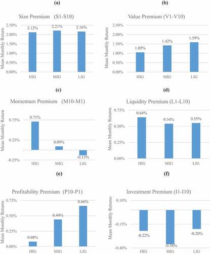
The size effect is observed for all the sample markets as small firm stocks generate higher returns than big firm stocks. Table 3 illustrates that the mean monthly size premium (S1-S10) is statistically significant, at 5% level, for 21 out of 25 countries. The highest monthly size premium is observed for Hong Kong (5.13%) followed by Egypt (3.84%), India (3.74%) and Australia (3.7%). In contrast, the size premium, though positive, is small for Israel (0.06%), Italy (0.11%) and Spain (0.22%). Further, mean returns, by and large, monotonically decline as one moves from small to big stock portfolios. The monthly global size premium stands at 2.16%, which is also significant. Thus, the universality of the size effect is reconfirmed as the mean size premium is statistically significant for all the three financial integration groups as well. Size effect does not seem to be impacted much by financial integration settings as the average premium is strong and almost similar across our integration groups.

Table 4 illustrates that the value premium (V1-V10) is positive for all markets except Israel. However, only 17 out of 25 markets exhibit a statistically significant value effect. High and significant value premiums are observed for Egypt (3.18%), India (2.70%), Indonesia (2.53%) and South Africa (2.02%). Israel reports the smallest value premium (−0.05%). The global monthly value premium is 1.36% which is also statistically significant. Globally, the value effect is comparatively weaker and provides a premium which is 63% of the size premium. The value effect becomes more robust as one moves from HIGs to LIGs. Further, the value effect is comparatively weaker than the size effect for HIG vis-a-vis LIG. It may be noted that the value premium is about 50% and 74% of the size premium for HIG and LIG.

Table 4. Unadjusted returns for value-sorted deciles

All Markets
	V1			V10			V1-V10
	Mean	t-stat		Mean	t-stat		Mean	t-stat
All Markets	.0231***	(11.79)		.0095***	(8.35)		.0136***	(8.45)
HIGH INTEGRATION GROUP
	V1			V10			V1-V10
	Mean	t-stat		Mean	t-stat		Mean	t-stat
USA	.0160***	(3.43)		.0119***	(3.44)		0.0041	(1.08)
UK	.0195***	(4.25)		.0074**	(2.12)		.0121***	(3.92)
France	.0171***	(3.09)		.0089***	(2.02)		.0082**	(2.15)
Germany	.0277***	(4.59)		0.0083	(1.67)		.0195***	(4.32)
Canada	.0273***	(4.35)		.0171***	(3.13)		0.0102	(1.91)
Sweden	.0170***	(3.27)		0.0090	(1.53)		0.0080	(1.79)
Australia	.0281***	(4.23)		.0128**	(2.24)		.0153***	(3.33)
Spain	0.0033	(.98)		−0.0036	(−1.08)		.0069**	(2.45)
Mean	.0195***	(6.17)		.0090***	(3.97)		.0105***	(5.64)
MEDIUM INTEGRATION GROUP
	V1			V10			V1-V10
	Mean	t-stat		Mean	t-stat		Mean	t-stat
Italy	0.0060	(1.03)		0.0019	(.35)		0.0042	(1.09)
MEDIUM INTEGRATION GROUP
	V1			V10			V1-V10
	Mean	t-stat		Mean	t-stat		Mean	t-stat
Singapore	.0266***	(3.66)		0.0090	(1.66)		.0176***	(3.53)
Hong Kong	.0299***	(3.89)		.0130**	(2.14)		.0170***	(2.64)
Brazil	.0242***	(3.13)		0.0131	(1.68)		0.0111	(1.61)
S.Korea	.0295***	(4.84)		.0188***	(3.41)		.0107**	(2.37)
S.Africa	.0326***	(5.13)		.0124**	(2.41)		.0202***	(3.95)
Taiwan	.0217***	(2.79)		0.0045	(.85)		.0172***	(2.84)
Japan	.0119***	(2.95)		0.0074	(1.90)		0.0045	(1.42)
Indonesia	.0375***	(4.41)		.0122**	(2.01)		.0253***	(3.76)
Mean	.0244***	(6.91)		.0103***	(5.67)		.0142***	(5.66)
LOW INTEGRATION GROUP
	V1			V10			V1-V10
	Mean	t-stat		Mean	t-stat		Mean	t-stat
India	.0431***	(3.81)		.0161**	(2.41)		.0270***	(3.10)
Thailand	.0257***	(4.62)		0.0082	(1.47)		.0176***	(4.26)
China	.0222***	(2.87)		.0168**	(2.27)		0.0054	(1.16)
LOW INTEGRATION GROUP
	V1			V10			V1-V10
	Mean	t-stat		Mean	t-stat		Mean	t-stat
Pakistan	.0314***	(3.73)		.0116**	(2.15)		.0199***	(2.68)
Malaysia	.0174***	(3.06)		0.0053	(1.49)		.0121***	(3.04)
Turkey	.0243***	(2.62)		0.0103	(1.19)		.0140***	(2.75)
Israel	0.0074	(1.73)		.0079**	(2.33)		−0.0005	(−.23)
Egypt	.0289***	(2.74)		−0.0029	(−.33)		.0318***	(4.33)
Mean	.0251***	(6.35)		.0092***	(3.85)		.0159***	(3.96)

For all 25 sample markets, return differentials are estimated by using corner portfolios (V1 and V10) based on price-to-book value. V1 and V10 indicate the smallest and largest value-sorted decile portfolios. ** and *** indicate significance at 5% level and 1% levels, respectively

Evidence on the momentum effect is mixed in the sample markets. Table 5 illustrates that nine out of twenty-five countries stocks’ register negative momentum premiums (M10-M1). The mean monthly global momentum premium is 0.22% which is not statistically significant. Significant momentum premiums are reported only in 4 out of 25 markets, namely, Australia (1.62%), Germany (1.42%), France (1.3%) and Thailand (1.14%). Thus the momentum anomaly seems to have faded over time for the majority of the world markets. Momentum premium is more pronounced and significant in the HIG markets and is recorded as 0.71% per month.

Table 5. Unadjusted Returns for Prior returns-sorted Deciles

All Markets
	M1			M10			M10-M1
	Mean	t-stat		Mean	t-stat		Mean	t-stat
All Markets	.0161***	(8.72)		.0183***	(9.99)		.0022	(1.48)
HIGH INTEGRATION GROUP
	M1			M10			M10-M1
	Mean	t-stat		Mean	t-stat		Mean	t-stat
USA	.0164***	(3.11)		.0200***	(4.36)		0.0036	(.67)
UK	0.0102	(1.82)		.0141***	(3.47)		0.0038	(.88)
France	0.0080	(1.29)		.0213***	(4.48)		.0133***	(2.77)
Germany	.0141**	(2.34)		.0283***	(5.81)		.0142***	(3.14)
Canada	.0281***	(4.18)		.0259***	(4.24)		−0.0023	(−.40)
Sweden	0.0133	(1.75)		.0157***	(2.92)		0.0024	(.39)
Australia	.0194**	(2.55)		.0356***	(5.14)		.0162***	(2.82)
Spain	0.0002	(.04)		0.0061	(1.53)		0.0059	(1.49)
Mean	.0137***	(4.41)		.0209***	(6.03)		.0071***	(2.86)
MEDIUM INTEGRATION GROUP
	M1			M10			M10-M1
	Mean	t-stat		Mean	t-stat		Mean	t-stat
Italy	0.0018	(.28)		0.0065	(1.37)		0.0047	(.90)
Singapore	0.0111	(1.37)		.0144**	(2.28)		0.0034	(.58)
Hong Kong	.0185**	(2.49)		.0211***	(2.78)		0.0026	(.40)
Brazil	.0184**	(1.99)		.0268***	(3.15)		0.0084	(1.10)
S.Korea	.0389***	(5.06)		.0275***	(3.09)		−0.0114	(−1.37)
S.Africa	.0222***	(3.60)		.0311***	(4.43)		0.0089	(1.37)
Taiwan	0.0131	(1.79)		0.0122	(1.92)		−0.0009	(−.16)
Japan	.0102**	(2.33)		.0110**	(2.51)		0.0008	(.19)
Indonesia	.0292***	(3.08)		.0207***	(3.13)		−0.0085	(−1.13)
Mean	.0181***	(4.64)		.0190***	(6.35)		0.0009	(.36)
LOW INTEGRATION GROUP
	M1			M10			M10-M1
	Mean	t-stat		Mean	t-stat		Mean	t-stat
India	.0278***	(2.75)		.0280***	(3.68)		0.0002	(.03)
Thailand	0.0107	(1.57)		.0221***	(3.46)		.0114**	(2.23)
China	.0171**	(2.14)		.0151**	(2.00)		−0.0019	(−.41)
Pakistan	.0280***	(3.37)		.0253***	(3.42)		−0.0026	(−.33)
Malaysia	0.0085	(1.55)		.0115**	(2.51)		0.0030	(.84)
Turkey	0.0160	(1.77)		0.0081	(.94)		−0.0079	(−1.63)
LOW INTEGRATION GROUP
	M1			M10			M10-M1
	Mean	t-stat		Mean	t-stat		Mean	t-stat
Israel	.0126**	(2.04)		0.0079	(1.92)		−0.0047	(−.80)
Egypt	0.0088	(.79)		0.0014	(.13)		−0.0075	(−.81)
Mean	.0162***	(5.46)		.0149***	(4.18)		−0.0013	(−.52)

For all 25 sample markets, return differentials are estimated by using corner portfolios (M1 and M10) based on 6-month prior returns. M1 and M10 indicate the smallest and largest prior returns-sorted decile portfolios. ** and *** indicate significance at 5% level and 1% levels, respectively

On the other hand, five out of eight LIG markets exhibit price reversals, and the mean monthly premium is −0.13%. The prior return patterns seem to vary for different financial integration settings as momentum is observable for HIG while mild contrarian behaviour is noticed in LIG markets. One possible reason for such price reversals could be that low-integrated markets may have higher proportion of volatile stocks, which can weaken the profitability of momentum-sorted portfolios (Lin et al., 2020). Another plausible explanation could be that, behaviourally, market participants in less integrated markets may be more prone to overreaction to bad news which results in a contrarian effect while participants in highly integrated markets could perhaps be more disposed towards underreaction to good news thus resulting in momentum effect (See Barberis et al., 1998; Chan et al. 1996). However, causes for differences in prior returns effect need further exploration.

The liquidity effect is visible across several sample markets as less liquid firms generate higher returns in most markets, consistent with Lee and Swaminathan (2000). Table 6 illustrates that the mean monthly global liquidity premium (L1-L10) is 58% and significant. A positive liquidity premium is observed for 20 sample countries, out of which it is significant only for seven markets. High monthly liquidity premiums are observed for Canada (2.44%), followed by India (2.36%) and France (1.47%). As in the case of the size effect, liquidity premiums do not differ much across our financial integration groups. Thus the liquidity anomaly doesnt seem to be highly pervasive and also not sensitive to the level of market integration.

Table 6. Unadjusted returns for liquidity-sorted deciles

All Markets
	L1			L10			L1-L10
	Mean	t-stat		Mean	t-stat		Mean	t-stat
All Markets	.0159***	(8.84)		.0101***	(9.74)		.0058***	(3.67)
HIGH INTEGRATION GROUP
	L1			L10			L1-L10
	Mean	t-stat		Mean	t-stat		Mean	t-stat
USA	.0136***	(4.49)		.0128***	(3.57)		0.0007	(.28)
UK	.0114***	(3.20)		0.0043	(1.14)		.0071***	(3.48)
France	.0210***	(4.75)		0.0063	(1.29)		.0147***	(3.18)
Germany	.0148***	(3.94)		0.0098	(1.85)		0.0051	(1.17)
Canada	.0337***	(5.31)		.0093**	(2.09)		.0244***	(4.22)
Sweden	0.0106	(1.33)		.0098**	(2.07)		0.0008	(.10)
Australia	.0129***	(2.67)		.0127**	(2.55)		0.0002	(.06)
Spain	0.0013	(.45)		0.0030	(.65)		−0.0017	(−.41)
Mean	.0149***	(4.22)		.0085***	(6.15)		0.0064	(1.89)
MEDIUM INTEGRATION GROUP
	L1			L10			L1-L10
	Mean	t-stat		Mean	t-stat		Mean	t-stat
Italy	−0.0028	(−.75)		0.0020	(.39)		−0.0049	(−1.25)
Singapore	.0176***	(3.00)		0.0042	(.64)		.0135**	(2.52)
Hong Kong	.0202***	(3.02)		0.0113	(1.87)		0.0089	(1.58)
Brazil	.0147***	(3.13)		.0164**	(2.11)		−0.0017	(−.24)
S.Korea	.0225***	(3.86)		.0212***	(3.85)		0.0014	(.32)
S.Africa	.0226***	(3.55)		.0113**	(2.12)		.0114**	(2.05)
Taiwan	.0141***	(2.75)		0.0055	(.95)		.0086**	(2.23)
Japan	.0084***	(3.15)		0.0076	(1.78)		0.0008	(.27)
Indonesia	.0249***	(6.06)		0.0144	(1.71)		0.0105	(1.25)
Mean	.0158***	(5.14)		.0104***	(4.73)		.0054**	(2.32)
LOW INTEGRATION GROUP
	L1			L10			L1-L10
	Mean	t-stat		Mean	t-stat		Mean	t-stat
India	.0385***	(5.06)		0.0149	(1.69)		.0236***	(3.29)
Thailand	.0114***	(4.46)		0.0114	(1.53)		0.0000	(.00)
China	.0194***	(2.63)		.0157**	(2.25)		0.0037	(.74)
Pakistan	.0159***	(3.61)		0.0120	(1.65)		0.0038	(.56)
Malaysia	.0115***	(3.14)		0.0075	(1.46)		0.0039	(1.15)
Turkey	.0168**	(2.24)		0.0184	(1.92)		−0.0016	(−.33)
LOW INTEGRATION GROUP
	L1			L10			L1-L10
	Mean	t-stat		Mean	t-stat		Mean	t-stat
Israel	0.0075	(1.93)		.0089***	(2.78)		−0.0014	(−.68)
Egypt	0.0146	(1.68)		0.0023	(.23)		0.0122	(1.28)
Mean	.0169***	(4.74)		.0114***	(5.89)		0.0055	(1.72)

For all 25 sample markets, return differentials are estimated by using corner portfolios (L1 and L10) based on average traded volume. L1 and L10 indicate the smallest and largest liquidity-sorted decile portfolios. ** and *** indicate significance at 5% level and 1% levels, respectively

Table 7 illustrates that positive profitability premiums are observed in 16 sample markets where highly profitable firms outperform weakly profitable firms, consistent with Fama and French (2008). Premiums for 6 (Pakistan, Thailand, Italy, Indonesia, Spain and France) of these 16 markets are statistically significant. The mean monthly global profitability premium is positive and significant at 0.39%. Nine markets exhibit small negative profitability premiums. This difference from Novy-Marx (2013) could be due to the use of gross profits as a measure of profitability and inclusion of only non-financial firms in their study sample while we use return-on-equity measure and also include the non-financial firms. Mean profitability premiums rise sharply from 0.08% to 0.66% as one moves from HIG to LIG markets. Thus, the profitability effect seems to be more pronounced for low-integrated markets. Geographically it is interesting to observe that LIG Asian economies generally exhibit profitability premiums while most MIG Asian economies report negative premiums.

Table 7. Unadjusted returns for profitability-sorted deciles

All Markets
	P1			P10			P10-P1
	Mean	t-stat		Mean	t-stat		Mean	t-stat
All Markets	.0142***	(8.22)		.0182***	(11.39)		.0039**	(2.12)
HIGH INTEGRATION GROUP
	P1			P10			P10-P1
	Mean	t-stat		Mean	t-stat		Mean	t-stat
USA	.0208***	(3.81)		.0108***	(3.96)		−.0100**	(−2.49)
UK	.0114**	(2.40)		.0123***	(3.75)		0.0010	(.33)
France	0.0088	(1.44)		.0202***	(3.77)		.0114***	(2.72)
Germany	0.0104	(1.63)		.0157***	(3.22)		0.0053	(1.16)
Canada	.0259***	(3.63)		.0157***	(3.76)		−.0101**	(−2.10)
Sweden	0.0096	(1.33)		.0161***	(3.51)		0.0065	(1.09)
Australia	.0302***	(3.85)		.0198***	(3.65)		−.0104**	(−1.96)
Spain	−0.0079	(−1.46)		0.0050	(1.24)		.0129***	(3.30)
Mean	.0136***	(3.03)		.0145***	(7.65)		0.0008	(.22)
MEDIUM INTEGRATION GROUP
	P1			P10			P10-P1
	Mean	t-stat		Mean	t-stat		Mean	t-stat
Italy	−0.0035	(−.54)		.0125**	(2.41)		.0160***	(3.61)
Singapore	0.0068	(.80)		.0114**	(2.04)		0.0046	(.80)
Hong Kong	.0208**	(2.44)		.0201***	(3.45)		−0.0008	(−.11)
Brazil	0.0160	(1.87)		.0163**	(2.49)		0.0003	(.06)
S.Korea	.0259***	(3.98)		.0233***	(4.14)		−0.0027	(−.54)
S.Africa	.0166**	(2.19)		.0278***	(4.01)		0.0113	(1.57)
Taiwan	0.0125	(1.67)		0.0088	(1.52)		−0.0037	(−.72)
Japan	.0104**	(2.30)		.0099**	(2.50)		−0.0006	(−.19)
Indonesia	.0153***	(2.67)		.0301***	(4.88)		.0148***	(3.09)
Mean	.0134***	(4.48)		.0178***	(6.35)		0.0044	(1.61)
LOW INTEGRATION GROUP
	P1			P10			P10-P1
	Mean	t-stat		Mean	t-stat		Mean	t-stat
India	.0217**	(2.26)		.0273***	(3.33)		0.0056	(.75)
Thailand	.0130**	(1.96)		.0309***	(4.40)		.0179***	(3.67)
China	.0226***	(2.78)		.0239***	(3.26)		0.0014	(.29)
Pakistan	0.0097	(1.21)		.0300***	(4.94)		.0203***	(3.29)
Malaysia	.0157***	(2.65)		.0100***	(2.61)		−0.0057	(−1.34)
Turkey	0.0149	(1.50)		.0224***	(2.74)		0.0076	(1.54)
LOW INTEGRATION GROUP
	P1			P10			P10-P1
	Mean	t-stat		Mean	t-stat		Mean	t-stat
Israel	.0145**	(2.30)		.0078**	(2.08)		−0.0066	(−1.43)
Egypt	0.0141	(1.14)		.0264**	(2.25)		0.0123	(.97)
Mean	.0158***	(9.63)		.0224***	(6.74)		0.0066	(1.74)

For all 25 sample markets, return differentials are estimated by using corner portfolios (P1 and P10) based on return on equity. P1 and P10 indicate the smallest and largest profitability-sorted decile portfolios. ** and *** indicate significance at 5% level and 1% levels, respectively

Further, all European economies, which are highly integrated, show positive premiums. In contrast to European markets, highly integrated countries of USA, Canada and Australia exhibit a negative profitability premium. The cross-sectional patterns in profitability premia need further attention in future research.

Except for Israel and Malaysia, other less integrated market investors seem to reward higher profitability stocks with higher returns. We see a clear distinction between European and non-European HIG markets in the case of profitability premium. All European markets have positive profitability premiums, while non-European markets like the USA, Canada and Australia show negative profitability premiums for our sample stocks over the last two decades.

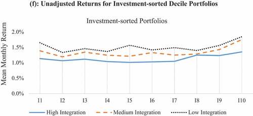
Table 8 illustrates that the investment effect, also called the asset growth effect, is found to be positive for nine markets, which is consistent with Fama & French, 2015) contention that low investment (conservative) firms outperform high investment (aggressive) firms. Only the USA out of these nine markets shows a significant investment effect. Majority of the markets, 16 out of 25, experience negative investment premium, 5 of which are statistically significant. The mean monthly global investment premium is negative (−0.26%) and statistically significant, thus implying aggressive stocks outperform conservative stocks. Interestingly, all European economies exhibit negative investment premiums. The net investment premiums are small and negative for all financial integration groups with little difference for HIG and LIG. Just like Foye (2018) and Gonenc and Ursu (2018), we too find that the asset-growth effect is mixed among our sample markets. One possible explanation for the positive relationship between asset growth and returns in various sample markets could be the idiosyncratic financing choices determined by institutional factors. In several markets, including EU and other emerging economies; bank financing is the dominant mode of fundraising (See Astrauskaite & Paškevicius, 2014; Langfield & Pagano, 2015), and it helps reduce agency costs associated with overinvestment through enhanced financial supervision (Harvey et al., 2004). Banks have better access to private information than bondholders in capital markets, who are more reliant on publicly available information (Fama, 1985). Banks have higher incentives to undertake information acquisition as they have large stakes in borrower funding (Boot et al., 1993). The empirical evidence on investment anomaly seems weak and tilted towards a negative investment premium. However, the factors leading to marginally superior returns in high asset growth firms from many sample markets require further examination.

Table 8. Unadjusted returns for investment-sorted deciles

All Markets
	I1			I10			I1-I10
	Mean	t-stat		Mean	t-stat		Mean	t-stat
All Markets	.0139***	(8.57)		.0165***	(11.87)		−.0026**	(−2.10)
HIGH INTEGRATION GROUP
	I1			I10			I1-I10
	Mean	t-stat		Mean	t-stat		Mean	t-stat
USA	.0177***	(4.42)		.0125***	(3.51)		.0052**	(2.09)
UK	.0083**	(2.04)		.0133***	(3.41)		−.0049**	(−2.19)
France	0.0089	(1.81)		.0144***	(2.73)		−0.0054	(−1.58)
Germany	.0130**	(2.33)		.0140***	(2.69)		−0.0011	(−.29)
Canada	.0191***	(3.22)		.0182***	(3.27)		0.0010	(.23)
Sweden	0.0092	(1.57)		0.0099	(1.70)		−0.0007	(−.18)
Australia	.0160***	(2.59)		.0207***	(3.07)		−0.0047	(−1.08)
Spain	−0.0016	(−.34)		0.0050	(1.11)		−0.0066	(−1.67)
Mean	.0113***	(4.50)		.0135***	(7.47)		−0.0022	(−1.43)
MEDIUM INTEGRATION GROUP
	I1			I10			I1-I10
	Mean	t-stat		Mean	t-stat		Mean	t-stat
Italy	−0.0017	(−.27)		.0112**	(2.31)		−.0129***	(−3.15)
Singapore	0.0043	(.61)		0.0129	(1.86)		−0.0086	(−1.78)
Hong Kong	.0256***	(3.01)		.0188***	(2.81)		0.0069	(1.09)
MEDIUM INTEGRATION GROUP
	I1			I10			I1-I10
	Mean	t-stat		Mean	t-stat		Mean	t-stat
Brazil	0.0126	(1.81)		.0156**	(2.16)		−0.0030	(−.54)
S.Korea	.0242***	(4.40)		.0236***	(3.87)		0.0006	(.12)
S.Africa	.0200***	(3.14)		.0280***	(4.53)		−0.0080	(−1.45)
Taiwan	.0152**	(2.22)		0.0105	(1.60)		0.0047	(1.05)
Japan	.0087**	(2.30)		.0089**	(2.11)		−0.0002	(−.10)
Indonesia	.0156***	(2.76)		.0279***	(4.05)		−.0123**	(−2.42)
Mean	.0138***	(4.34)		.0175***	(6.62)		−0.0036	(−1.43)
LOW INTEGRATION GROUP
	I1			I10			I1-I10
	Mean	t-stat		Mean	t-stat		Mean	t-stat
India	.0308***	(3.42)		.0276***	(2.92)		0.0032	(.47)
Thailand	.0220***	(2.83)		.0149**	(2.52)		0.0072	(1.09)
China	.0212***	(2.65)		.0248***	(3.23)		−0.0036	(−1.00)
Pakistan	0.0126	(1.90)		.0272***	(4.08)		−.0146***	(−3.01)
Malaysia	.0145***	(2.71)		.0111**	(2.42)		0.0034	(.89)
Turkey	0.0130	(1.50)		.0206**	(2.44)		−.0075**	(−2.20)
Israel	.0129**	(2.00)		0.0110	(1.88)		0.0020	(.36)
Egypt	0.0045	(.47)		0.0102	(.93)		−0.0057	(−.72)
Mean	.0164***	(5.46)		.0184***	(6.48)		−0.0020	(−.72)

For all 25 sample markets, return differentials are estimated by using corner portfolios (I1 and I10) based on change in total assets in previous period. I1 and I10 indicate the smallest and largest investment rate-sorted decile portfolios. ** and *** indicate significance at 5% level and 1% levels, respectively

To sum up the study of average monthly unadjusted returns, we find that size and value effect are the dominant effects and offer the highest returns. Size premium, at 2.16% per month, is highest among the six anomalies analysed across all sample markets, followed by the value premium at 1.35% p.m. The momentum effect weans out at low levels of integration, suggesting that momentum strategy is better suited for HIG markets. A statistically significant liquidity premium is observed only in MIG markets. The profitability effect is more visible in the less integrated markets, and the investment effect is not observed in either of the integration groups.⁷

We try to explain these anomaly premium patterns across financial integration groups through prior literature. It is observed that size and liquidity premia are quite similar across all three integration groups (Table 9). Small size and low liquidity firms are generally neglected and have relatively lower coverage by analysts from investment advisory companies. The stocks with poor analyst coverage tend to have higher transaction costs and lower liquidity (Dang et al., 2019). As these phenomena are pretty universal in nature we observe similar size and value premia across all integration groups. In case of other anomalies like value (price-to-book value) and profitability (return on equity), the reaction of investors to new accounting-based information could be different in HIG and LIG markets. Many LIG markets are also emerging markets, which are more sentiment-driven and investors may be prone to an overreaction (Ahmad & Hussain, 2001; Tripathi & Gupta, 2009; Wu, 2011) to accounting-based information leading to higher premiums, unlike the more mature markets (Clare & Thomas, 1995).

The global mean monthly returns on six market anomalies are shown in Figure 1. The size effect is dominant in the world markets, followed by the value and liquidity effects. The momentum, profitability and asset growth anomalies are weak for global markets. Further small firms, low price-to-book value and less liquid stocks outperform big firms, high price-to-book value firms for most of the sample markets. Momentum patterns are observed for HIG markets, while most LIG markets exhibit weak contrarian behaviour. The profitability effect is more pronounced in LIG markets. The evidence on asset-growth anomaly is mixed, and mildly negative premiums are observed across all financial integration-based market groups.

Figure 1. Mean returns on decile portfolios.(a) unadjusted returns for size-sorted decile portfolios.(b) unadjusted returns for value-sorted decile portfolios.(c) unadjusted returns for momentum-sorted decile portfolios.(d) unadjusted returns for liquidity-sorted decile portfolios.(e) unadjusted returns for profitability-sorted decile portfolios.(f) unadjusted returns for investment-sorted decile portfolios.

Note: S1 to S10 indicates the smallest to largest size-sorted decile portfolios.

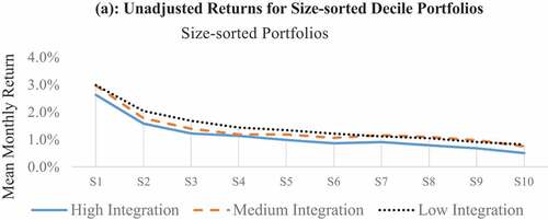
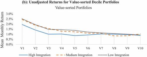
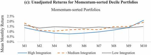
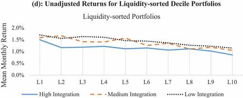
Figure 1. Continued.

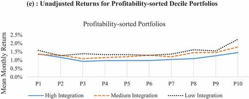
Figure 2 illustrates mean monthly premiums for the six market anomalies across different financial integration groups. More financially integrated economies tend to provide lower value and profitability premiums than less integrated markets. Momentum patterns are stronger for more integrated markets. Size, liquidity and investment premiums do not vary much across varying financial integration settings.

Figure 2. Return differentials on decile portfolios in three financial integration groups.

Note: The figures indicate the mean monthly return differentials on characteristic-sorted corner portfolios for high, medium and low integration group markets. HIG, MIG and LIG represent high, medium and low integration group of markets, respectively.

Mean monthly return differentials on characteristic-sorted corner portfolios for all 25 sample markets and their significance is presented as a heat map in Figure 3. It contains the performance of equity market anomalies across the sample countries. France reports the most significant anomalies, i.e. 5 out of 6, the only exception being the investment effect. Five markets i.e. Australia, UK, Thailand, Pakistan and Indonesia, exhibit four significant anomalies. Size, profitability, and investment effects are significant for the US market. No significant anomaly is observed for Israel, while only the size effect seems strong in the case of Brazil. The heat map provides vital information to global investors regarding making market choices for designing anomaly based trading strategies in different markets. More integrated markets report a higher number of significant anomalies (25 out of 48) compared to less integrated markets (18 out of 48). A part of this result may be explained by the fact that some of the low-integrated economies have high market risk, and they catch much lower investor attention, leading to limited and infrequent trading in many financial assets from these markets.

Figure 3. Return differentials on market anomalies for sample countries.

Note: For size premium, we calculate the difference between small (S1) and big firm (S10) stock returns. In the case of the value effect, we take the difference between low (V1) and high PB stocks (V10). For prior returns, past losers (M1) are subtracted from past winners (M10). Similarly, liquidity premium is the difference between low liquidity (L1) and high liquidity (L10) stocks, while profitability effect is the difference between high profitable (P10) and low profitable (P1) firms. Finally, the investment premium is estimated as the difference between low investment (I1) and high investment (I10) companies.*(+) values denote that return differentials are positive and significant at 5% level. *(-) values imply that return differ entials are negative and statistically significant at 5% level Blank represents return differential values which are not statistically significant

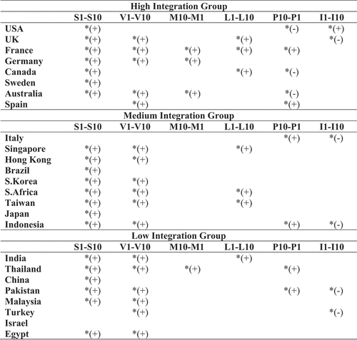
In sum, we confirm that returns on value, momentum (prior returns) and profitability anomalies vary across financial integration groups. As against this, size, liquidity and asset growth effects are not dissimilar for markets exhibiting different levels of financial integration. Using paired t-test, we examine if the difference in anomaly premiums between low and high integration groups are statistically significant. The t-test statistics, contained in Table 10 support evidence of significant differences in the average value premium of HIG and LIG returns at a 5% level of significance. There is also a significant difference in mean monthly premiums for prior returns and profitability at a 10% level of significance. No significant difference is observed in the mean monthly premiums for size, liquidity and investment-sorted portfolios.

Table 9. Mean monthly return differentials on characteristic-sorted corner portfolios

	Size (S1-S10)	Value (V1-V10)	Momentum (M10-M1)	Liquidity (L1-L10)	Profitability (P10-P1)	Investment (I1-I10)
All Markets	0.0216***	0.0135***	0.0022	0.0058***	0.0039**	−0.0026**
(t-stat)	(8.73)	(8.45)	(1.48)	(3.67)	(2.12)	(−2.11)
HIG (t-stat)	0.0212***	0.0105***	0.0071**	0.0064	0.0008	−0.0022
	(5.29)	(5.64)	(2.86)	(1.89)	(0.22)	(−1.43)
MIG (t-stat)	0.0221***	0.0142***	0.0009	0.0054**	0.0044	−0.0036
	(4.71)	(5.66)	(0.36)	(2.32)	(1.61)	(−1.43)
LIG (t-stat)	0.0216***	0.0159***	−0.0013	0.0055	0.0066	−0.002
	(4.12)	(3.96)	(−0.52)	(1.72)	(1.74)	(−0.72)

Panel A contains return differentials that are estimated by using corner portfolios (decile one and decile ten) based on each company characteristic. For size premium, we calculate the difference between small (S1) and big firm (S10) stock returns. In the case of the value effect, we take the difference between low (V1) and high PB stocks (V10). For prior returns, past losers (M1) are subtracted from past winners (M10). In the case of momentum (M10-M1) exhibit a positive sign while a negative sign implies price reversals. Similarly, liquidity premium is the difference between low liquidity (L1) and high liquidity (L10) stocks, while profitability effect is the difference between high profitable (P10) and low profitable (P1) firms. Investment premium is estimated as the difference between low investment (I1) and high investment (I10) companies. ** and *** indicate significance at 5% level and 1% levels, respectively.

Table 10. Testing for significance in risk and return

	(1)	(2)	(3)	(4)	(5)
	Integration Groups	Return Mean	t-test p-value	Return Volatility	F-test p-value
Size	HIG	0.0212	0.893	0.0377	0.129
	LIG	0.0216		0.0418
Value	HIG	0.0159	0.041**	0.0376	0.990
	LIG	0.0158		0.0375
Momentum	HIG	0.0013	0.069*	0.0503	0.108
	LIG	0.0000		0.0451
Liquidity	HIG	0.0055	0.655	0.0352	0.000***
	LIG	0.0039		0.0525
Profitability	HIG	0.0066	0.096*	0.0366	0.128
	LIG	0.0059		0.0406
Investment	HIG	−0.0020	0.651	0.0235	0.000***
	LIG	−0.0027		0.0405

Mean monthly return differentials on characteristic-sorted corner portfolios for high, medium and low integration group markets are estimated from corner portfolios (decile one and decile ten) for high and low integration group markets. The premium series is created by assigning equal weights to each market. We apply t-test to check for significant differences in mean return series of high and low integration markets. Similarly, to test for differences in risk, estimated by standard deviation, we apply F-test. *, ** and *** indicate significance at 10%, 5% level and 1% levels, respectively.

We next verify if cross-sectional differences in anomaly based premiums may be an outcome of differences in mean characteristics for corner portfolios, the results for which are reported in Table 11. We find a weak association between return premiums and characteristic differences for our sample markets, as shown by low correlation values. Thus, we confirm that differences in company attributes are not a significant driver of cross-sectional differences in premiums. Prior research cites other important drivers of cross-sectional premiums such as financial market development, leverage constraints, information uncertainty, and idiosyncratic volatility (See Black, 1972; Frazzini and Pedersen, 2014; Bali, 2017).

Table 11. Correlation between characteristic and return premiums

PANEL A
HIGH INTEGRATION GROUP
	Size	Value	Momentum	Liquidity	Profitability	Investment
USA	4.17	7.68	0.13	4.13	61.11	0.80
UK	5.63	6.63	0.13	6.59	65.11	0.92
France	6.47	5.65	0.14	10.88	56.41	0.82
Germany	7.40	5.46	0.17	9.97	64.23	0.87
Canada	5.90	5.32	0.21	6.81	70.00	1.21
Sweden	7.32	6.77	0.21	8.43	92.74	1.21
Australia	7.32	7.37	0.24	6.96	87.77	1.31
Spain	8.46	6.52	0.14	11.41	70.96	1.01
MEDIUM INTEGRATION GROUP
	Size	Value	Momentum	Liquidity	Profitability	Investment
Italy	7.09	5.14	0.16	9.27	68.22	0.87
Singapore	6.17	4.36	0.24	7.39	65.04	1.01
Hong Kong	6.69	6.00	0.24	6.20	82.97	1.27
Brazil	11.49	6.46	0.17	13.16	84.83	1.05
S.Korea	5.60	3.89	0.12	6.75	58.40	0.81
S.Africa	8.39	6.16	0.26	8.96	79.21	1.12
Taiwan	4.79	4.23	0.23	5.30	46.97	0.76
Japan	3.82	3.77	0.22	5.09	31.39	0.42
Indonesia	6.66	5.88	0.17	11.17	65.10	0.89
LOW INTEGRATION GROUP
	Size	Value	Momentum	Liquidity	Profitability	Investment
India	5.20	8.09	0.23	6.90	62.85	0.95
Thailand	5.67	4.72	0.22	10.32	63.91	0.78
China	4.64	6.46	0.17	3.77	43.45	0.97
Pakistan	8.62	5.70	0.28	10.73	73.43	0.86
Malaysia	5.70	4.00	0.16	6.48	53.59	0.77
Turkey	6.77	4.61	0.21	7.71	77.38	1.04
Israel	3.83	7.67	0.11	3.80	81.98	1.02
Egypt	6.33	5.59	0.28	8.89	64.26	0.81
PANEL B
	Size	Value	Momentum	Liquidity	Profitability	Investment
All Country	0.02	−0.05	0.22	0.03	0.21	0.02

Panel A includes the absolute mean characteristic differences of corner portfolios. The characteristic differences are calculated for corner portfolios (decile one and decile ten). For size and volume log values have been taken. So, the characteristic premium for price-to-book (PB) value is the absolute difference between average PB for decile one (V1) and decile ten (V10) companies.

Panel B shows association between the correlations between absolute values of characteristic differences and absolute return premiums.

Investors looking to profit from value and profitability-based strategies should prefer LIG markets as the equally weighted mean premiums are significantly higher than HIG markets. Investors who prefer momentum strategy should focus on the eight HIG markets as returns and significantly higher than LIG markets. However, mean monthly premiums on size, illiquidity and investment-sorted portfolios do not vary with the level of financial integration. So premiums for size, liquidity and investment are not significantly different across the integration groups.

In the next sub-section, we examine the role of alternative asset pricing models in explaining returns on our anomaly based portfolios. We also evaluate the efficacy of local versus global risk factors on the cross-section of returns. Finally, we verify the explanatory power of these risk models under varying financial integration settings.

6.3. Performance of asset pricing models

In the final stage, we evaluate the performance multifactor asset pricing models on the 1500 domestic portfolios (60 portfolios for our 25 sample markets) using local and world factors. Three asset pricing models have been used as performance benchmarks, namely, one-factor L-CAPM, involving the local market factor, Fama-French three-factor model (L-FF-3) involving market, size, and value factors and Fama-French five-factor models (L-FF-5), which include profitability and investment factors in addition to local FF-3 factors. Three variants of each model are employed in the study: a local factor model, a world factor version, and a hybrid model, which comprises local and foreign factors. The factor construction procedure has been explained in Section 3 along the lines of Griffin (2002). The model equations are provided in Appendix I.

We evaluate the performance of three versions of CAPM (See equations (1)(1) ${\mathrm{x}}_{\mathrm{t}}={\sum }_{i=1}^p{\mathrm{\Phi }}_i{x}_{t-i}+{\epsilon }_t$(1) , (2(2) ${\theta }_{ij}^g\left(H\right)=\frac{{{\sigma }_{ii}}^{-1}{\sum }_{h=0}^{H-1}(e{ }_i^{\prime }{A}_h{\sum }^{e_j}){ }^2}{{\sum }_{h=0}^{H-1}(e{ }_i^{\prime }{A}_h{\sum }^A{ }_h^{\prime }{e}_j){ }^{\hspace{0.17em}}}$(2) ), and (3(3) ${\theta }_{ij\hspace{0.17em}}^g\left(H\right)=\hspace{0.17em}\frac{{\theta }_{ij\hspace{0.17em}}^g\left(H\right)}{{\sum }_{j=1}^N{\theta }_{ij\hspace{0.17em}}^g\left(H\right)}$(3) ) in Appendix I) on the sample portfolios. Table 12 shows the asset pricing results for local factors using three versions of CAPM. One factor CAPM results show that the market factor plays an important role in explaining security returns. Betas are significant for the sample portfolios, and adjusted R² is 0.685 on an overall basis. The size and value factors also make an important contribution in explaining returns as the adjusted R² is 0.765 for the L-FF-3 factor model. The role of profitability and investment factors in the cross-section of returns seems limited as only 1.7% is added to the explanatory power of the L-FF-3 factor model, and adjusted R² is reported to be 0.782. There seems to be no significant difference in the results of alternative finance integration groups. The L-FF-5 factor model appears to be the best descriptor of asset returns with local factors.

Table 12. Goodness-of-fit of alternative asset pricing benchmarks using local factors

ALL MARKETS
	L-CAPM			L-FF-3			L-FF-5
	α	adj-R^2		α	adj-R^2		α	adj-R^2
All Markets	0.007	0.685		0.004	0.765		0.004	0.782
HIGH INTEGRATION GROUP
	L-CAPM			L-FF-3			L-FF-5
	α	adj-R^2		α	adj-R^2		α	adj-R^2
USA	0.008	0.738		0.002	0.837		0.002	0.859
UK	0.008	0.767		0.002	0.860		0.001	0.870
France	0.009	0.711		0.006	0.769		0.006	0.781
Germany	0.007	0.682		0.003	0.758		0.002	0.774
Canada	0.009	0.681		0.004	0.759		0.004	0.770
Sweden	0.006	0.629		0.003	0.720		0.004	0.745
Australia	0.011	0.752		0.004	0.817		0.004	0.830
Spain	0.003	0.560		0.002	0.606		0.003	0.642
Mean	0.007	0.690		0.003	0.766		0.003	0.784
MEDIUM INTEGRATION GROUP
	L-CAPM			L-FF-3			L-FF-5
	α	adj-R^2		α	adj-R^2		α	adj-R^2
Italy	0.004	0.726		0.003	0.788		0.003	0.798
Singapore	0.004	0.699		0.004	0.798		0.004	0.816
Hong Kong	0.011	0.562		0.003	0.704		0.002	0.716
MEDIUM INTEGRATION GROUP
	L-CAPM			L-FF-3			L-FF-5
	α	adj-R^2		α	adj-R^2		α	adj-R^2
Brazil	0.005	0.678		0.003	0.740		0.003	0.754
S.Korea	0.015	0.667		0.011	0.707		0.011	0.724
S.Africa	0.008	0.634		0.005	0.686		0.004	0.707
Taiwan	0.006	0.792		0.003	0.891		0.003	0.898
Japan	0.005	0.820		0.002	0.883		0.002	0.891
Indonesia	0.010	0.632		0.004	0.718		0.003	0.730
Mean	0.008	0.690		0.004	0.768		0.004	0.782
LOW INTEGRATION GROUP
	L-CAPM			L-FF-3			L-FF-5
	α	adj-R^2		α	adj-R^2		α	adj-R^2
India	0.010	0.823		0.006	0.861		0.007	0.887
Thailand	0.008	0.659		0.003	0.744		0.003	0.772
China	0.010	0.738		0.002	0.863		0.002	0.866
Pakistan	0.007	0.577		0.004	0.646		0.005	0.673
Malaysia	0.004	0.677		0.003	0.802		0.002	0.818
Turkey	0.006	0.825		0.005	0.873		0.006	0.880
Israel	0.005	0.596		0.006	0.657		0.005	0.695
Egypt	0.007	0.506		0.008	0.640		0.006	0.664
Mean	0.007	0.675		0.005	0.761		0.005	0.782

Three local factor models are used to explain the cross-section of portfolio returns, namely, local CAPM (L-CAPM), local Fama-French three-factor model (L-FF-3) and local Fama-French five-factor model (L-FF-5). The goodness of fit of these alternative asset pricing models is verified by comparing their mean adj-R². Models with higher mean adj-R² provide a better explanation of the cross-section of returns. The mean absolute alpha values have also been reported for these models.

Next, we evaluate the power of multifactor models in explaining sample country portfolios using our value-weighted (market cap) world factors (See equations 4(4) $\mathbf{L}-\mathbf{F}\mathbf{F}-\mathbf{3}:{\mathrm{R}}_{\mathrm{p}\mathrm{t}}--{\mathrm{R}}_{\mathrm{f}\mathrm{t}}=\alpha +\beta \left({\mathrm{R}}_{\mathrm{m}\mathrm{t}}--{\mathrm{R}}_{\mathrm{f}\mathrm{t}}\right)+\mathrm{s}\left(\mathrm{S}\mathrm{M}{\mathrm{B}}_{\mathrm{t}}\right)+\mathrm{h}\left(\mathrm{L}\mathrm{M}{\mathrm{H}}_{\mathrm{t}}\right)+{\epsilon }_{\mathrm{t}}$(4) , 5(5) $\mathbf{W}-\mathbf{F}\mathbf{F}-\mathbf{3}:{\mathrm{R}}_{\mathrm{p}\mathrm{t}}--{\mathrm{R}}_{\mathrm{f}\mathrm{t}}=\alpha +{\beta }_{\mathrm{w}}\left(\mathrm{W}{\mathrm{R}}_{\mathrm{m}\mathrm{t}}--{\mathrm{R}}_{\mathrm{f}\mathrm{t}}\right)+{\mathrm{s}}_{\mathrm{w}}\left(\mathrm{W}\mathrm{S}\mathrm{M}{\mathrm{B}}_{\mathrm{t}}\right)+{\mathrm{h}}_{\mathrm{w}}\left(\mathrm{W}\mathrm{L}\mathrm{M}{\mathrm{H}}_{\mathrm{t}}\right)+{\epsilon }_{\mathrm{t}}$(5) , and 6(6) $\begin{array}{rl}& \mathbf{H}-\mathbf{F}\mathbf{F}-\mathbf{3}:{\mathrm{R}}_{\mathrm{p}\mathrm{t}}--{\mathrm{R}}_{\mathrm{f}\mathrm{t}}=\alpha +\beta \left({\mathrm{R}}_{\mathrm{m}\mathrm{t}}--{\mathrm{R}}_{\mathrm{f}\mathrm{t}}\right)+\mathrm{s}\left(\mathrm{S}\mathrm{M}{\mathrm{B}}_{\mathrm{t}}\right)+\mathrm{h}\left(\mathrm{L}\mathrm{M}{\mathrm{H}}_{\mathrm{t}}\right)\\ & +{\beta }_{\mathrm{f}}\left(\mathrm{F}{\mathrm{R}}_{\mathrm{m}\mathrm{t}}--{\mathrm{R}}_{\mathrm{f}\mathrm{t}}\right)+{\mathrm{s}}_{\mathrm{f}}\left(\mathrm{F}\mathrm{S}\mathrm{M}{\mathrm{B}}_{\mathrm{t}}\right)+{\mathrm{h}}_{\mathrm{f}}\left(\mathrm{F}\mathrm{L}\mathrm{M}{\mathrm{H}}_{\mathrm{t}}\right)+{\epsilon }_{\mathrm{t}}\end{array}$(6) in Appendix I). Table 13 illustrates results for goodness of fit of asset pricing models using world factors. We observe that world factor models underperform local factor asset pricing models. However, the multifactor versions perform better than one-factor world CAPM (W-CAPM) on an overall basis. W-CAPMs mean goodness of fit for all countries is 0.422, while W-FF-3 and W-FF-5 are marginally better at explaining returns with adj-R² of 0.444 and 0.452, respectively. We also observe that with the addition of Fama-French (FF) world factors to W-CAPM, the incremental performance of W-FF-3 and W-FF-5 models vis-à-vis local FF factor models is not so pronounced in all three integration settings.

Table 13. Goodness-of-fit of alternative asset pricing benchmarks using world factors

All Markets
	W-CAPM			W-FF-3			W-FF-5
	α	adj-R^2		α	adj-R^2		α	adj-R^2
All Markets	0.010	0.422		0.006	0.444		0.006	0.452
HIGH INTEGRATION GROUP
	W-CAPM			W-FF-3			W-FF-5
	α	adj-R^2		α	adj-R^2		α	adj-R^2
USA	0.008	0.671		0.003	0.722		0.004	0.739
UK	0.006	0.648		0.004	0.705		0.004	0.707
France	0.007	0.619		0.003	0.641		0.004	0.648
Germany	0.008	0.639		0.003	0.651		0.003	0.654
Canada	0.011	0.503		0.003	0.570		0.003	0.579
Sweden	0.008	0.513		0.005	0.557		0.003	0.566
Australia	0.012	0.601		0.004	0.619		0.004	0.624
Spain	0.002	0.387		0.005	0.408		0.007	0.415
Mean	0.008	0.573		0.004	0.609		0.004	0.616
MEDIUM INTEGRATION GROUP
	W-CAPM			W-FF-3			W-FF-5
	α	adj-R^2		α	adj-R^2		α	adj-R^2
Italy	0.003	0.553		0.006	0.562		0.007	0.562
Singapore	0.004	0.556		0.005	0.567		0.009	0.579
MEDIUM INTEGRATION GROUP
	W-CAPM			W-FF-3			W-FF-5
	α	adj-R^2		α	adj-R^2		α	adj-R^2
Hong Kong	0.012	0.426		0.005	0.471		0.008	0.493
Brazil	0.009	0.407		0.006	0.425		0.007	0.427
S.Korea	0.019	0.408		0.013	0.414		0.011	0.415
S.Africa	0.013	0.395		0.009	0.397		0.007	0.400
Taiwan	0.007	0.279		0.004	0.304		0.005	0.309
Japan	0.005	0.382		0.002	0.401		0.001	0.399
Indonesia	0.016	0.348		0.009	0.364		0.007	0.369
Mean	0.010	0.417		0.006	0.434		0.007	0.439
LOW INTEGRATION GROUP
	W-CAPM			W-FF-3			W-FF-5
	α	adj-R^2		α	adj-R^2		α	adj-R^2
India	0.016	0.428		0.011	0.427		0.005	0.436
Thailand	0.013	0.210		0.006	0.221		0.004	0.245
China	0.014	0.220		0.004	0.237		0.003	0.234
Pakistan	0.016	0.048		0.012	0.056		0.014	0.052
LOW INTEGRATION GROUP
	W-CAPM			W-FF-3			W-FF-5
	α	adj-R^2		α	adj-R^2		α	adj-R^2
Malaysia	0.007	0.356		0.003	0.371		0.004	0.372
Turkey	0.010	0.369		0.005	0.371		0.015	0.431
Israel	0.007	0.399		0.002	0.435		0.004	0.446
Egypt	0.006	0.177		0.015	0.202		0.018	0.197
Mean	0.011	0.276		0.007	0.290		0.008	0.302

In world CAPM (WCAPM), portfolio returns are regressed on the world market factor. In W-FF-3 factor model, portfolio returns are regressed on the world market, size and value factors. While in W-FF-5 factor model, we use world profitability and investment factors in explaining asset returns. Results are only shown for value-weighted world factors. The goodness of fit of these alternative asset pricing models is verified by comparing their mean adj-R². Models with higher mean adj-R² provide a better explanation of the cross-section of returns. The mean absolute alpha values have also been reported for these models.

Comparing results across financial integration groups, one finds that the world factor models perform best for highly integrated economies followed by MIG and LIG. The mean adj-R² for W-FF-5 are found to be 0.616, 0.439, 0.302 for HIG, MIG, and LIG markets. These findings are consistent with the premise that world factors shall play a more important role in economies that are more globalised and integrated than economies that are relatively less open. Our asset pricing results seem to vary with different financial integration settings.

Lastly, we employ hybrid models comprising of both local and value-weighted foreign factors (See Equations 7(7) $\begin{array}{rl}& \mathbf{L}-\mathbf{F}\mathbf{F}-\mathbf{5}:{\mathrm{R}}_{\mathrm{p}\mathrm{t}}--{\mathrm{R}}_{\mathrm{f}\mathrm{t}}=\alpha +\beta \left({\mathrm{R}}_{\mathrm{m}\mathrm{t}}--{\mathrm{R}}_{\mathrm{f}\mathrm{t}}\right)+\mathrm{s}\left(\mathrm{S}\mathrm{M}{\mathrm{B}}_{\mathrm{t}}\right)\\ & +\mathrm{h}\left(\mathrm{L}\mathrm{M}{\mathrm{H}}_{\mathrm{t}}\right)+\mathrm{r}\left(\mathrm{R}\mathrm{M}{\mathrm{W}}_{\mathrm{t}}\right)+\mathrm{c}\left(\mathrm{C}\mathrm{M}{\mathrm{A}}_{\mathrm{t}}\right)+{\epsilon }_{\mathrm{t}}\end{array}$(7) ,8(8) $\begin{array}{rl}& \mathbf{W}-\mathbf{F}\mathbf{F}-\mathbf{5}:{\mathrm{R}}_{\mathrm{p}\mathrm{t}}--{\mathrm{R}}_{\mathrm{f}\mathrm{t}}=\alpha +\beta \left(\mathrm{W}{\mathrm{R}}_{\mathrm{m}\mathrm{t}}--{\mathrm{R}}_{\mathrm{f}\mathrm{t}}\right)+{\mathrm{s}}_{\mathrm{w}}\left(\mathrm{W}\mathrm{S}\mathrm{M}{\mathrm{B}}_{\mathrm{t}}\right)\\ & +{\mathrm{h}}_{\mathrm{w}}\left(\mathrm{W}\mathrm{L}\mathrm{M}{\mathrm{H}}_{\mathrm{t}}\right)+{\mathrm{r}}_{\mathrm{w}}\left(\mathrm{W}\mathrm{R}\mathrm{M}{\mathrm{W}}_{\mathrm{t}}\right)+{\mathrm{c}}_{\mathrm{w}}\left(\mathrm{W}\mathrm{C}\mathrm{M}{\mathrm{A}}_{\mathrm{t}}\right)+{\epsilon }_{\mathrm{t}}\end{array}$(8) and 9(9) $\begin{array}{rl}& \mathbf{H}-\mathbf{F}\mathbf{F}-\mathbf{5}:{\mathrm{R}}_{\mathrm{p}\mathrm{t}}--{\mathrm{R}}_{\mathrm{f}\mathrm{t}}=\alpha +\beta \left({\mathrm{R}}_{\mathrm{m}\mathrm{t}}--{\mathrm{R}}_{\mathrm{f}\mathrm{t}}\right)+\mathrm{s}\left(\mathrm{S}\mathrm{M}{\mathrm{B}}_{\mathrm{t}}\right)\\ & +\mathrm{h}\left(\mathrm{L}\mathrm{M}{\mathrm{H}}_{\mathrm{t}}\right)+\mathrm{r}\left(\mathrm{R}\mathrm{M}{\mathrm{W}}_{\mathrm{t}}\right)+\mathrm{c}\left(\mathrm{C}\mathrm{M}{\mathrm{A}}_{\mathrm{t}}\right)+{\beta }_{\mathrm{f}}\left(\mathrm{F}{\mathrm{R}}_{\mathrm{m}\mathrm{t}}--{\mathrm{R}}_{\mathrm{f}\mathrm{t}}\right)\\ & +{\mathrm{s}}_{\mathrm{f}}\left(\mathrm{F}\mathrm{S}\mathrm{M}{\mathrm{B}}_{\mathrm{t}}\right)+{\mathrm{h}}_{\mathrm{f}}\left(\mathrm{F}\mathrm{L}\mathrm{M}{\mathrm{H}}_{\mathrm{t}}\right)+{\mathrm{r}}_{\mathrm{f}}\left(\mathrm{F}\mathrm{R}\mathrm{M}{\mathrm{W}}_{\mathrm{t}}\right)+{\mathrm{c}}_{\mathrm{f}}\left(\mathrm{F}\mathrm{C}\mathrm{M}{\mathrm{A}}_{\mathrm{t}}\right)+{\epsilon }_{\mathrm{t}}\end{array}$(9) in Appendix I). Table 14 illustrates results for performance of assets pricing models using hybrid factors. One may recall that foreign factors do not include the weighted returns for the local market whose portfolio returns are being evaluated, unlike the world factors. H-CAPM model includes local and foreign market factors. Similarly, we have the H-FF-3 factor model which has additional local and foreign Fama-French factors for size and value. The H-FF-5 factor model has local and foreign factors for profitability and investment added to the H-FF-3 factor model.

Table 14. Goodness-of-fit of alternative asset pricing benchmarks using hybrid factors

All Markets
	H-CAPM			H-FF-3			H-FF-5
	α	adj-R^2		α	adj-R^2		α	adj-R^2
All Markets	0.008	0.693		0.005	0.776		0.005	0.795
HIGH INTEGRATION GROUP
	H-CAPM			H-FF-3			H-FF-5
	α	adj-R^2		α	adj-R^2		α	adj-R^2
USA	0.008	0.745		0.003	0.840		0.003	0.863
UK	0.008	0.768		0.002	0.864		0.002	0.873
France	0.008	0.718		0.003	0.790		0.002	0.804
Germany	0.007	0.703		0.003	0.777		0.004	0.793
Canada	0.010	0.685		0.002	0.777		0.002	0.794
Sweden	0.006	0.637		0.004	0.741		0.004	0.768
Australia	0.011	0.756		0.003	0.826		0.003	0.839
Spain	0.003	0.564		0.004	0.629		0.005	0.686
Mean	0.007	0.697		0.003	0.781		0.003	0.803
MEDIUM INTEGRATION GROUP
	H-CAPM			H-FF-3			H-FF-5
	α	adj-R^2		α	adj-R^2		α	adj-R^2
Italy	0.003	0.733		0.003	0.798		0.002	0.808
Singapore	0.010	0.823		0.006	0.862		0.005	0.888
Hong Kong	0.011	0.566		0.007	0.722		0.010	0.747
Brazil	0.005	0.679		0.006	0.746		0.007	0.760
S.Korea	0.015	0.668		0.011	0.708		0.011	0.724
S.Africa	0.008	0.635		0.005	0.688		0.004	0.708
Taiwan	0.006	0.794		0.005	0.893		0.005	0.900
Japan	0.005	0.826		0.002	0.886		0.002	0.894
Indonesia	0.010	0.632		0.005	0.725		0.006	0.739
Mean	0.008	0.706		0.005	0.781		0.006	0.796
LOW INTEGRATION GROUP
	H-CAPM			H-FF-3			H-FF-5
	α	adj-R^2		α	adj-R^2		α	adj-R^2
India	0.010	0.823		0.006	0.862		0.005	0.888
Thailand	0.008	0.659		0.004	0.747		0.003	0.775
China	0.010	0.738		0.003	0.863		0.003	0.865
Pakistan	0.007	0.576		0.005	0.649		0.008	0.677
Malaysia	0.004	0.688		0.003	0.814		0.003	0.827
Turkey	0.006	0.826		0.006	0.875		0.006	0.881
LOW INTEGRATION GROUP
	H-CAPM			H-FF-3			H-FF-5
	α	adj-R^2		α	adj-R^2		α	adj-R^2
Israel	0.005	0.597		0.002	0.677		0.002	0.718
Egypt	0.007	0.504		0.012	0.641		0.011	0.665
Mean	0.007	0.676		0.005	0.766		0.005	0.787

Hybrid factor models use both local and foreign factors to explain portfolio returns. For hybrid CAPM (H-CAPM), the two factors are foreign and local market factors. H-FF3 factor model includes six factors, i.e. local and foreign market, size and value factors. The H-FF-5 factor model has four additional factors for profitability and investment (both local and foreign). Results are only shown for value-weighted foreign factors. The goodness of fit of these alternative asset pricing models is verified by comparing their mean adj-R². Models with higher mean adj-R² provide a better explanation of the cross-section of returns. The mean absolute alpha values have also been reported for these models.

Overall, the performance of hybrid models is superior to both local and world factor models. Mean goodness of fit for all markets are H-CAPM, H-F F-3 and H-FF-5 are 0.693, 0.776 and 0.795, respectively, which are higher than counterpart local and world factor models. The FF foreign factors add a 1.3% additional variance of asset returns compared to FF-5 local factors.

We find that hybrid, H-FF-5, model performs better than all the competing models across the three integration groups. As expected, foreign factors do the best job for highly integrated economies. The foreign factors provide an additional explanation of asset returns to the tune of 1.9%, 1.5% and 0.5% for HIG, MIG and LIG. Putting it all together, H-FF-5 seems to be the most suitable descriptor of asset pricing for high and medium integrated markets. For low-integrated markets, the contribution of foreign factors is marginal. Since the contribution of foreign factors is marginal, one can employ the L-FF-5 model as the performance benchmark for LIG markets, owing to its parsimonious factor structure.

After adjusting for degrees of freedom, the additional foreign factors incrementally explain domestic returns by about 1%. However, the superior performance of hybrid models vis-à-vis local factor models varies considerably across integration groups. The highest incremental explanation by foreign factors is registered in the case of MIG and HIG markets, while it is the least for LIG markets. Model-wise too, the highest incremental explanation of almost 2% is recorded from local FF-5 to hybrid FF-5 model in HIG markets. This is along expected lines as foreign factors do not contribute much in explaining returns for LIG markets. So we find H-FF-5 factor model to be the most suitable model for HIG and MIG markets, while the local FF-5 model seems adequate for LIG.

The absolute values of mean alphas are reported for one-factor CAPM and multifactor models (See Table 12–14). We observe that alphas are lower for multifactor models when compared to alphas for one-factor CAPM. The alphas lower when we use local or hybrid factor models as compared to those of world factor models and thus confirm the efficacy of local and hybrid factor models in explaining the variance in portfolio returns. Within integration groups, the mean absolute alpha values for HIG markets are comparatively smaller than those of LIG markets. This is observed for all three types of factor models-local (Table 12), world (Table 13), and hybrid (Table 14). These low alphas imply smaller mispricing errors and hence confirm the predictive superiority of multifactor models. This also confirms lower mispricing errors in multifactor models.

7. Robustness tests

We perform robustness tests to confirm that our results are not an outcome of specific estimation procedures. We redevelop the financial integration index using forty-month, instead of the thirty-month, rolling window of returns and conditional volatility. We observe no change in the classification of the HIG, MIG, and LIG markets.

We constructed decile portfolios in the main study. As a robustness check, we also construct quintile portfolios to evaluate if our anomaly based returns are sensitive to alternative portfolio formation procedures. We did not find evidence of significant differences in anomaly premiums for quintile and decile portfolio formations. Hence our results are robust for portfolio construction procedures as illustrated in Appendix III table. We also reconstruct our world and foreign factors using equal-weights instead of value-weights. Asset pricing tests are repeated using equally weighted versions of world factor models. We also test hybrid models involving equally weighted foreign factors. The results based on equally weighted factor models are similar to those for value-weighted factor models, reported earlier in the study. These findings are consistent with Griffin (2002). Thus, our asset pricing results are robust for alternative factor-weighing procedures.⁸

8. Conclusion

In this study, we focus on the performance of key equity market anomalies and evaluate the ability of alternative asset pricing benchmarks’ ability to explain such anomalies under different financial integration settings.

We find that size is the most dominant anomaly in world markets followed by value and liquidity. Value and profitability effects are stronger for less integrated markets. Highly integrated markets exhibit short-term momentum while mild reversals are prominent in low-integrated markets. Global investment premia are negative, implying that high investment firms outperform low investment firms in several of our sample markets. A significant difference in the mean monthly premiums for value, prior returns and profitability are observed between HIG and LIG markets. However, no such significant differences exist for mean monthly size, illiquidity and investment premiums of HIG and LIG markets. Our findings have strong implications for the current market classification system and related market efficiency arguments. Performance of market anomalies seems to vary more with financial integration classification than with “developed” and “emerging” market segregation criteria. Global investors could use “financial integration” as an additional framework for categorising financial markets to generate significantly higher returns. Portfolio managers can generate superior returns through value and profitability-based strategies in low integration markets, while HIG markets can offer them significantly higher momentum premiums. A size-based investment strategy can be used across all markets.

We further evaluate the power of single and alternative multifactor models in explaining returns and find that the Fama-French five-factor model is a better descriptor of asset returns than the CAPM and Fama-French three-factor model. Local factor models work well for low-integrated markets. International factors are relevant, besides local factors, only in the case of more integrated markets. So, local factors should be augmented with international factors in the Fama-French five-factor model framework to evaluate more integrated market portfolios. We recommend the local factor FF-5 model as the performance benchmark for less integrated markets due to its parsimonious factor structure.

We conclude that the performance of equity market anomalies and asset pricing benchmarks varies under different integration settings. We offer a new framework to global investors for portfolio selection as well as performance evaluation. Ignoring the aspect of financial integration in asset pricing can result in compromised investment strategies with sub-optimal portfolio selection.

Disclosure statement

No potential conflict of interest was reported by the author(s).

Notes

1. Morgan Stanley classifies the countries into “Developed”, “Emerging” and “Frontier and Standalone” Markets.

2. In asset pricing domain, anomalies are seen as abnormalities which cannot be explained by multi-factor models as they violate the risk-return relationship. Prominent anomalies like firm size, value, momentum have a rich literature, but studies on profitability, investment and liquidity are thin, especially for emerging markets. Section two discusses literature review about market anomalies.

3. Investment effect or the asset growth effect means higher returns are generated by firms which are conservative in investing.

4. These 47 markets are USA, UK, Netherlands, France, Germany, Canada, Sweden, Australia, Switzerland, Denmark, Mexico, Norway, Belgium, Spain, Austria, Italy, Singapore, Hong Kong, Brazil, South Korea, South Africa, Finland, Hungary, Taiwan, Portugal, Japan, Czech Republic, Russia, Chile, New Zealand, Indonesia, India, Greece, Thailand, Peru, China, Pakistan, Malaysia, Poland, Argentina, Turkey, Sri Lanka, Israel, Philippines, Colombia, Egypt, Jordan.

5. See IMF Paper titled Recovery from the Asian Crisis and the Role of the IMF by IMF Staff, June 2000 https://www.imf.org/external/np/exr/ib/2000/062300.htm#I

6. Table 2 illustrates that HIG countries: United States, UK, France, Germany, Canada, Sweden, Australia, Spain; MIG countries: Italy, Singapore, Hong Kong, Brazil, South Korea, South Africa, Taiwan, Japan, Indonesia; LIG countries: India, Thailand, China, Pakistan, Malaysia, Turkey, Israel, Egypt.

7. Due to space constraints, Tables 3–8 contain results only for the decile corner portfolios. Results from second to ninth decile portfolios can be made available on request.

8. Robustness test results are not included in the paper owing to paucity of space and can be made available upon request.

Appendix I:

Equations of asset pricing tests

We use different asset pricing frameworks for testing the three asset pricing models, namely, CAPM, Fama-French three-factor model (FF-3) and Fama-French five-factor model (FF-5). Sample market portfolios are tested on empirical asset pricing models. 5 different asset pricing frameworks are used for testing the three asset pricing models:

(1) local factor(s)

(2) value-weighted world factor(s)

(3) local factors and value-weighted foreign factor(s)

(4) equally weighted world factors

(5) local factors and equally weighted foreign factor(s)

CAPM test on domestic portfolios use local, world, and hybrid market factor models:

(1) $\mathbf{L}-\mathbf{C}\mathbf{A}\mathbf{P}\mathbf{M}:{\mathrm{R}}_{\mathrm{p}\mathrm{t}}--{\mathrm{R}}_{\mathrm{f}\mathrm{t}}=\alpha +\beta \left({\mathrm{R}}_{\mathrm{m}\mathrm{t}}--{\mathrm{R}}_{\mathrm{f}\mathrm{t}}\right)+{\epsilon }_{\mathrm{t}}$(1)

(2) $\mathbf{W}-\mathbf{C}\mathbf{A}\mathbf{P}\mathbf{M}:{\mathrm{R}}_{\mathrm{p}\mathrm{t}}--{\mathrm{R}}_{\mathrm{f}\mathrm{t}}=\alpha +{\beta }_{\mathrm{w}}\left(\mathrm{W}{\mathrm{R}}_{\mathrm{m}\mathrm{t}}--{\mathrm{R}}_{\mathrm{f}\mathrm{t}}\right)+{\epsilon }_{\mathrm{t}}$(2)

(3) $\mathbf{H}-\mathbf{C}\mathbf{A}\mathbf{P}\mathbf{M}:{\mathrm{R}}_{\mathrm{p}\mathrm{t}}--{\mathrm{R}}_{\mathrm{f}\mathrm{t}}=\alpha +\beta \left({\mathrm{R}}_{\mathrm{m}\mathrm{t}}--{\mathrm{R}}_{\mathrm{f}\mathrm{t}}\right)+{\beta }_{\mathrm{f}}\left(\mathrm{F}{\mathrm{R}}_{\mathrm{m}\mathrm{t}}--{\mathrm{R}}_{\mathrm{f}\mathrm{t}}\right)+{\epsilon }_{\mathrm{t}}$(3)

where

R_pt—R_ft  = mean excess monthly domestic portfolio return

R_mt—R_ft  = local market index mean excess return

WR_mt—R_ft  = world market mean excess return (equal-weighted and value-weighted)

FR_mt—R_ft  = foreign market mean excess return (equal-weighted and value-weighted)

ε_t  = error term at a given time “t”

β  = slope of the market factor representing the sensitivity of market factor

β_w = slope of the market factor representing the sensitivity of, equal-weighted and value-weighted, World market factors

β_f = slope of the market factor representing the sensitivity of, equal-weighted and value-weighted, foreign market factor

α  = intercept or the Αlpha

The world factors and foreign factors used in this study are equal weighted or value weighted on market cap. Value-weighted factors are created using Griiffin (2002) methodology. For example world market factor is the weighted average of the local market-specific components. So WR_mt = wL_t-1R_mt + wF_t−1 FR_mt, where wL_t−1 is the market cap weight (w) of the local market (L) in all sample countries market for the previous period (t-1). wF_t−1 is the fraction of the total market capitalization in the previous period attributable to foreign market capitalization. The world SMB, LMH, RWM, CMA factors are also weighted averages of their respective local factors.

Fama and French (1993) three factor model additionally uses the additional “size” and “value” factors to explain the portfolio returns. Size and Value factors constructed too are local, world and hybrid in nature

(4) $\mathbf{L}-\mathbf{F}\mathbf{F}-\mathbf{3}:{\mathrm{R}}_{\mathrm{p}\mathrm{t}}--{\mathrm{R}}_{\mathrm{f}\mathrm{t}}=\alpha +\beta \left({\mathrm{R}}_{\mathrm{m}\mathrm{t}}--{\mathrm{R}}_{\mathrm{f}\mathrm{t}}\right)+\mathrm{s}\left(\mathrm{S}\mathrm{M}{\mathrm{B}}_{\mathrm{t}}\right)+\mathrm{h}\left(\mathrm{L}\mathrm{M}{\mathrm{H}}_{\mathrm{t}}\right)+{\epsilon }_{\mathrm{t}}$(4)

(5) $\mathbf{W}-\mathbf{F}\mathbf{F}-\mathbf{3}:{\mathrm{R}}_{\mathrm{p}\mathrm{t}}--{\mathrm{R}}_{\mathrm{f}\mathrm{t}}=\alpha +{\beta }_{\mathrm{w}}\left(\mathrm{W}{\mathrm{R}}_{\mathrm{m}\mathrm{t}}--{\mathrm{R}}_{\mathrm{f}\mathrm{t}}\right)+{\mathrm{s}}_{\mathrm{w}}\left(\mathrm{W}\mathrm{S}\mathrm{M}{\mathrm{B}}_{\mathrm{t}}\right)+{\mathrm{h}}_{\mathrm{w}}\left(\mathrm{W}\mathrm{L}\mathrm{M}{\mathrm{H}}_{\mathrm{t}}\right)+{\epsilon }_{\mathrm{t}}$(5)

(6) $\begin{array}{rl}& \mathbf{H}-\mathbf{F}\mathbf{F}-\mathbf{3}:{\mathrm{R}}_{\mathrm{p}\mathrm{t}}--{\mathrm{R}}_{\mathrm{f}\mathrm{t}}=\alpha +\beta \left({\mathrm{R}}_{\mathrm{m}\mathrm{t}}--{\mathrm{R}}_{\mathrm{f}\mathrm{t}}\right)+\mathrm{s}\left(\mathrm{S}\mathrm{M}{\mathrm{B}}_{\mathrm{t}}\right)+\mathrm{h}\left(\mathrm{L}\mathrm{M}{\mathrm{H}}_{\mathrm{t}}\right)\\ & +{\beta }_{\mathrm{f}}\left(\mathrm{F}{\mathrm{R}}_{\mathrm{m}\mathrm{t}}--{\mathrm{R}}_{\mathrm{f}\mathrm{t}}\right)+{\mathrm{s}}_{\mathrm{f}}\left(\mathrm{F}\mathrm{S}\mathrm{M}{\mathrm{B}}_{\mathrm{t}}\right)+{\mathrm{h}}_{\mathrm{f}}\left(\mathrm{F}\mathrm{L}\mathrm{M}{\mathrm{H}}_{\mathrm{t}}\right)+{\epsilon }_{\mathrm{t}}\end{array}$(6)

where

SMB_t  = difference between returns on small size portfolio and big size portfolio

LMH_t  = difference between returns on low value and high value portfolios

WSMB_t  = equal-weighted and value weighted world size factor constructed from difference between returns of small size and big size portfolios of all 25 markets

WLMH_t  = equal-weighted and value weighted world value factor constructed from difference between returns of small value and big value portfolios of all 25 markets

FSMB_t  = equal-weighted and value weighted foreign size factor constructed from difference between returns of small size and big size portfolios of 24 markets

FLMH_t  = equal-weighted and value weighted foreign value factor constructed from difference between returns of small value and big value portfolios of 24 markets

ε_t  = error term at a given time “t”

s = coefficients of small minus big (SMB) factor

h = coefficients of low minus high (LMH) factor

s_w  = coefficients of world SMB factor

h_w  = coefficients of world LMH factor

s_f  = coefficients of foreign SMB factors

h_f  = coefficients of foreign LMH factors

The Fama & French, 2015) five factor model frameworks used in the study are given below. This model, in addition to FF-3 factors, uses the local, world and hybrid factors for profitability and investment.

(7) $\begin{array}{rl}& \mathbf{L}-\mathbf{F}\mathbf{F}-\mathbf{5}:{\mathrm{R}}_{\mathrm{p}\mathrm{t}}--{\mathrm{R}}_{\mathrm{f}\mathrm{t}}=\alpha +\beta \left({\mathrm{R}}_{\mathrm{m}\mathrm{t}}--{\mathrm{R}}_{\mathrm{f}\mathrm{t}}\right)+\mathrm{s}\left(\mathrm{S}\mathrm{M}{\mathrm{B}}_{\mathrm{t}}\right)\\ & +\mathrm{h}\left(\mathrm{L}\mathrm{M}{\mathrm{H}}_{\mathrm{t}}\right)+\mathrm{r}\left(\mathrm{R}\mathrm{M}{\mathrm{W}}_{\mathrm{t}}\right)+\mathrm{c}\left(\mathrm{C}\mathrm{M}{\mathrm{A}}_{\mathrm{t}}\right)+{\epsilon }_{\mathrm{t}}\end{array}$(7)

(8) $\begin{array}{rl}& \mathbf{W}-\mathbf{F}\mathbf{F}-\mathbf{5}:{\mathrm{R}}_{\mathrm{p}\mathrm{t}}--{\mathrm{R}}_{\mathrm{f}\mathrm{t}}=\alpha +\beta \left(\mathrm{W}{\mathrm{R}}_{\mathrm{m}\mathrm{t}}--{\mathrm{R}}_{\mathrm{f}\mathrm{t}}\right)+{\mathrm{s}}_{\mathrm{w}}\left(\mathrm{W}\mathrm{S}\mathrm{M}{\mathrm{B}}_{\mathrm{t}}\right)\\ & +{\mathrm{h}}_{\mathrm{w}}\left(\mathrm{W}\mathrm{L}\mathrm{M}{\mathrm{H}}_{\mathrm{t}}\right)+{\mathrm{r}}_{\mathrm{w}}\left(\mathrm{W}\mathrm{R}\mathrm{M}{\mathrm{W}}_{\mathrm{t}}\right)+{\mathrm{c}}_{\mathrm{w}}\left(\mathrm{W}\mathrm{C}\mathrm{M}{\mathrm{A}}_{\mathrm{t}}\right)+{\epsilon }_{\mathrm{t}}\end{array}$(8)

(9) $\begin{array}{rl}& \mathbf{H}-\mathbf{F}\mathbf{F}-\mathbf{5}:{\mathrm{R}}_{\mathrm{p}\mathrm{t}}--{\mathrm{R}}_{\mathrm{f}\mathrm{t}}=\alpha +\beta \left({\mathrm{R}}_{\mathrm{m}\mathrm{t}}--{\mathrm{R}}_{\mathrm{f}\mathrm{t}}\right)+\mathrm{s}\left(\mathrm{S}\mathrm{M}{\mathrm{B}}_{\mathrm{t}}\right)\\ & +\mathrm{h}\left(\mathrm{L}\mathrm{M}{\mathrm{H}}_{\mathrm{t}}\right)+\mathrm{r}\left(\mathrm{R}\mathrm{M}{\mathrm{W}}_{\mathrm{t}}\right)+\mathrm{c}\left(\mathrm{C}\mathrm{M}{\mathrm{A}}_{\mathrm{t}}\right)+{\beta }_{\mathrm{f}}\left(\mathrm{F}{\mathrm{R}}_{\mathrm{m}\mathrm{t}}--{\mathrm{R}}_{\mathrm{f}\mathrm{t}}\right)\\ & +{\mathrm{s}}_{\mathrm{f}}\left(\mathrm{F}\mathrm{S}\mathrm{M}{\mathrm{B}}_{\mathrm{t}}\right)+{\mathrm{h}}_{\mathrm{f}}\left(\mathrm{F}\mathrm{L}\mathrm{M}{\mathrm{H}}_{\mathrm{t}}\right)+{\mathrm{r}}_{\mathrm{f}}\left(\mathrm{F}\mathrm{R}\mathrm{M}{\mathrm{W}}_{\mathrm{t}}\right)+{\mathrm{c}}_{\mathrm{f}}\left(\mathrm{F}\mathrm{C}\mathrm{M}{\mathrm{A}}_{\mathrm{t}}\right)+{\epsilon }_{\mathrm{t}}\end{array}$(9)

Where

RMW_t  = difference in returns on local portfolios with high and low profitability i.e. robust profitability minus weak profitability

CMAt  = difference in returns on portfolios with low and high investment, i.e. returns of firms with conservative investment minus aggressive investment firms

WRMW_t  = equal-weighted and value weighted world profitability factor created from difference between returns of high and low profitability firms of all 25 markets

WCMA_t  = equal-weighted and value weighted world investment factor created difference between returns of low and high investment firms of all 25 markets

FRMW_t = equal-weighted and value weighted foreign profitability factor created from difference between returns of high and low profitability firms of all 24 markets

FCMA_t = equal-weighted and value weighted foreign investment factor which is difference between returns of low and high investment firms of all 24 markets

r = coefficients of robust minus weak (RMW) factor

c = coefficients of conservative minus aggressive (CMA) factor

r_w   = coefficients of world RMW factor

c_w  = coefficients of world CMA factor

r_f   = coefficients of foreign RMW factor

c_f  = coefficients of foreign CMA factor

Appendix II:

Testing for stationarity

Table below includes the results of stationarity tests. We use the Augmented Dickey Fuller Test to confirm stationarity out our time series for benchmark indices and company share prices, for each of the 25 markets and the world market.

Table

	At Level		At First Difference
Country Index	Augmented Dickey Fuller Test statistic (Test critical values at 5% level is −3.4)	Probability	Augmented Dickey Fuller Test statistic	Probability
Australia	−2.1	0.5	−13.7	0.0
Brazil	−1.5	0.8	−13.1	0.0
Canada	−2.2	0.5	−13.5	0.0
China	−2.9	0.2	−12.9	0.0
Egypt	−1.8	0.7	−13.0	0.0
France	−2.1	0.5	−14.1	0.0
Germany	−2.3	0.4	−13.7	0.0
Hong Kong	−2.7	0.2	−13.4	0.0
India	−2.6	0.3	−14.3	0.0
Indonesia	−2.2	0.5	−13.2	0.0
Israel	−2.1	0.5	−14.1	0.0
Italy	−1.7	0.8	−13.2	0.0
Japan	−1.7	0.8	−14.1	0.0
Malaysia	−1.7	0.8	−13.2	0.0
Pakistan	−1.8	0.7	−13.6	0.0
Singapore	−2.4	0.4	−14.1	0.0
S. Africa	−2.6	0.3	−15.8	0.0
S. Korea	−2.5	0.3	−14.2	0.0
Spain	−1.8	0.7	−13.2	0.0
Sweden	−2.3	0.5	−13.7	0.0
Taiwan	−2.5	0.3	−14.9	0.0
Thailand	−2.8	0.2	−14.7	0.0
Turkey	−2.6	0.3	−15.0	0.0
UK	−2.0	0.6	−14.1	0.0
USA	−0.7	1.0	−15.4	0.0
World	−1.5	0.8	−14.0	0.0

Appendix III: Testing for partition sensitivity between decile and quintile portfolios

Table below includes the results from testing portfolio partition sensitivity. We conducted a t-test between the mean monthly premium time series for integration groupings, of all six anomalies, derived from decile (10) and quintile-partitioned (10) portfolios. We also measured the correlations between decile and quintile portfolios’ anomaly premium times series. Table below includes the t-test and correlation results for anomaly premiums from decile and quintile portfolios

Table

Decile and quintile-sorted portfolios
	HIG		MIG		LIG
	p-value	Correlation	p-value	Correlation	p-value	Correlation
Size	0.070	0.95	0.020	0.94	0.133	0.88
Value	0.399	0.95	0.480	0.94	0.263	0.91
Momentum	0.511	0.96	0.806	0.95	0.811	0.94
Liquidity	0.378	0.95	0.897	0.91	0.859	0.96
Profitability	0.981	0.93	0.684	0.93	0.546	0.88
Investment	0.551	0.88	0.910	0.93	0.910	0.88

References

- Aharon, D. Y., & Qadan, M. (2019). The size effect is alive and well, and hiding behind calendar anomalies. The Journal of Portfolio Management, 45(6), 61–51. https://doi.org/10.3905/jpm.2019.1.088
- Aharoni, G., Grundy, B., & Zeng, Q. (2013). Stock returns and the miller modigliani valuation formula: Revisiting the Fama French analysis. Journal of Financial Economics, 110, 347–357. https://doi.org/10.1016/j.jfineco.2013.08.003
- Ahmad, Z., & Hussain, S. (2001). KLSE long run overreaction and the Chinese new-year effect. Journal of Business Finance and Accounting, 28(1–2), 63–105. https://doi.org/10.1111/1468-5957.00366
- Akbari, A., Ng, L., & Solnik, B. (2020). Emerging markets are catching up: economic or financial integration? Journal of Financial and Quantitative Analysis, 1–34. https://doi.org/10.1017/S0022109019000681
- Alquist, R., Israel, R., & Moskowitz, T. (2018). Fact, fiction, and the size effect. The Journal of Portfolio Management, 45(1), 34–61. https://doi.org/10.3905/jpm.2018.1.082
- Amihud, Y., & Mendelson, H. (1986). Asset pricing and the Bid-ask spread. Journal of Financial Economics, 17, 223–249. https://doi.org/10.1016/0304-405X(86)90065-6
- Antoniou, A., Lam, H. Y., & Paudyal, K. (2007). Profitability of momentum strategies in international markets: The role of business cycle variables and behavioural biases. Journal of Banking and Finance, 31(3), 955–972. https://doi.org/10.1016/j.jbankfin.2006.08.001
- Artmann, S., Finter, P., & Kempf, A. (2011). Determinants of expected stock returns: Large sample evidence from the German market. CFR Working Paper, 10–11[rev.], University of Cologne, Centre for Financial Research (CFR).
- Astrauskaite, I., & Paškevicius, A. (2014). Competition between banks and bond markets: Hardly impacted or softly complemented. Procedia Economics and Finance, 9, 111–119. https://doi.org/10.1016/S2212-5671(14)00012-4
- Ayuso, J., & Blanco, R. (2001). Has financial market integration increased during the nineties? Journal of International Financial Markets, Institutions and Money, 11(3–4), 265–287. https://doi.org/10.1016/S1042-4431(01)00036-1
- Bali, T. G., Brown, S. J., Murray, S., & Tang, Y. (2017). A lottery-demand-based explanation of the beta anomaly. Journal of Financial and Quantitative Analysis, 52(6), 2369–2397. https://doi.org/10.1017/S0022109017000928
- Banz, R. W. (1981). The relationship between return and market value of common stock. Journal of Financial Economics, 3–18. https://doi.org/10.1016/0304-405X(81)90018-0
- Barberis, N., Shliefer, A., & Vishny, R. (1998). A model of investor sentiment. Journal of Financial Economics, 49, 307–343. https://doi.org/10.1016/S0304-405X(98)00027-0
- Bekaert, G., & Harvey, C. R. (1995). Time-varying world market integration. Journal of Finance, 50(2), 403–444. https://doi.org/10.1111/j.1540-6261.1995.tb04790.x
- Bekaert, G., Harvey, C. R., & Lumsdaine, R. L. (2002). Dating the integration of world equity market. Journal of Financial Economics, 65, 203–247. https://doi.org/10.1016/S0304-405X(02)00139-3
- Bekaert, G., Harvey, C., Lundblad, C, R., & Siegel, S. (2011). What segments equity markets. Review of Financial Studies, 3841–3890. https://doi.org/10.1093/rfs/hhr082
- Bekaert, G., Harvey, C., Lundblad, C, R., & Siegel, S. (2013). The European Union, the Euro, and equity market Integration. Journal of Financial Economics, 109, 583–603. https://doi.org/10.1016/j.jfineco.2013.03.008
- Black, F. (1972). Capital market equilibrium with restricted borrowing. Journal of Business, Pages, 45(3), 444–455. https://doi.org/10.1086/295472
- Boot, A., Greenbaum, S., & Thakor, A. (1993). Reputation and discretion in financial contracting. American Economic Review, 83(5), 1165–1183. http://www.jstor.org/stable/2117554
- Cakici, N., Fabozzi, F. J., & Tan, S. (2013). Size, value, and momentum in emerging market stock returns. Emerging Markets Review, 16, 46–65. https://doi.org/10.1016/j.ememar.2013.03.001
- Chan, K. C., & Chen, N. F. (1991). Structural and return characteristics of small and large firms. The Journal of Finance, 46(4), 1467–1484. https://doi.org/10.1111/j.1540-6261.1991.tb04626.x
- Chan, C., Chen, N., & Hseih. (1985). An exploratory investigation of the firm size effect. Journal of Financial Economics, 14, 451–471. https://doi.org/10.1016/0304-405X(85)90008-X
- Chen, T., Sun, L., Wei, K. C. J., & Xie, F. (2018). The profitability effect: Insights from international equity markets. European Financial Management, 24(4), 545–580. https://doi.org/10.1111/eufm.12189
- Chiang, T. C., & Zheng, D. (2015). Liquidity and stock returns: Evidence from international markets. Global Finance Journal, 27, 73–97. https://doi.org/10.1016/j.gfj.2015.04.005
- Chordia, T., & Shivakumar, L. (2002). Momentum, business cycle and time varying expected returns. The Journal of Finance, 57(2), 985–1019. https://doi.org/10.1111/1540-6261.00449
- Chui, A., Titman, S., & Wei, K. (2010). Individualism and momentum around the world. The Journal of Finance, LXV(1), 361–392. https://doi.org/10.1111/j.1540-6261.2009.01532.x
- Clare, A., & Thomas, S. (1995). The overreaction hypothesis and the UK stock market. Journal of Business Finance and Accounting, 22(7), 961–973. https://doi.org/10.1111/j.1468-5957.1995.tb00888.x
- Cohen, R. B., Gompers, P. A., & Vuolteenaho, T. (2002). Who underreacts to cashflow news? evidenec from trading between individuals and institutions. Journal of Financial Economics, 66, 409–462. https://doi.org/10.1016/S0304-405X(02)00229-5
- Cooper, M., Gulen, H., & Schill, M. (2008). Asset growth and the cross- section of stock returns. Journal of Finance, 63, 1609–1651. https://doi.org/10.1111/j.1540-6261.2008.01370.x
- Crain, M. A. (2011). A literature review of the size effect. Working Paper, Florida Atlantic University.
- Dang, T. L., Doan, N. T. P., Nguyen, T. M. H., Tran, T. T., & Vo, X. V. (2019). Analysts and stock liquidity – Global evidence. Cogent Economics & Finance, 7(1), 1–27. https://doi.org/10.1080/23322039.2019.1625480
- De Bondt, W. F., & Thaler, R. (1987). Further evidence of investor overreaction and stock market seasonality. The Journal of Finance, 42, 557–581. https://doi.org/10.1111/j.1540-6261.1987.tb04569.x
- Diebold, F. X., & Yilmaz, K. (2012). Better to give than to receive: Predictive directional measurement of volatility spillovers. International Journal of Forecasting, 28(1), 57–66. https://doi.org/10.1016/j.ijforecast.2011.02.006
- Dimson, E., Marsh, P., & Staunton, M. (2017). Factor-based investing: The long-term evidence. The Journal of Portfolio Management, 43(5), 15–37. Special QES Issue. https://doi.org/10.3905/jpm.2017.43.5.015
- Drew, M. E., Marsden, A., & Veeraraghavan, M. (2006). Small firm effect, liquidity and security returns: Australian evidence. Journal of Emerging Market Finance, 5(2), 135–149. https://doi.org/10.1177/097265270600500202
- Eichengreen, B. (2001). Capital Account Liberalization: What Do Cross-Country Studies Tell Us? World Bank. Washington, DC: World Bank. https://openknowledge.worldbank.org/handle/10986/17435
- Evans, J. L., & Archer, S. H. (1968). Diversification and the reduction of dispersion: An empirical analysis. The Journal of Finance, 23(5), 761–767. https://doi.org/10.1111/j.1540-6261.1968.tb00315.x
- Fama, E. (1985). What’s different about banks? Journal of Monetary Economics, 15, 29–39. https://doi.org/10.1016/0304-3932(85)90051-0
- Fama, E., & French, K. (1992). The cross-section of expected returns. The Journal of Finance, 47(2), 427–465. https://doi.org/10.1111/j.1540-6261.1992.tb04398.x
- Fama, E., & French, K. (1996). Multifactor expalnation of asset pricing anomalies. The Journal of Finance, 51, 55–84. https://doi.org/10.1111/j.1540-6261.1996.tb05202.x
- Fama, E., & French, K. (2008). Dissecting anomalies. The Journal of Finance, 63(4), 1653–1678. https://doi.org/10.1111/j.1540-6261.2008.01371.x
- Fama, E., & French, K. (2012). Size, value, and momentum in international stock returns. Journal of Financial Economics, 105, 457–472. https://doi.org/10.1016/j.jfineco.2012.05.011
- Fama, E., & French, K. (2015). A five-factor asset pricing model. Journal of Financial Economics, 116, 1–22. https://doi.org/10.1016/j.jfineco.2014.10.010
- Fama, E., & French, K. (2017). International tests of a five-factor asset pricing model. Journal of Financial Economics, 123(3), 441–463. https://doi.org/10.1016/j.jfineco.2016.11.004
- Fitzpatrick, J., & Ogden, J. P. Do asset pricing anomalies have a common link? an empirical analysis of interactions among failure risk proxies, external financing, and stock returns (March 18, 2009). https://ssrn.com/abstract=1364888
- Foye, J. (2018). A comprehensive test of the Fama-French five-factor model in emerging markets. Emerging Markets Review, 37, 199–222. https://doi.org/10.1016/j.ememar.2018.09.002
- Frazzini, A., & Pedersen, L. H. (2014). Betting against beta. Journal of Financial Economics, 111(1), 1–25. https://doi.org/10.1016/j.jfineco.2013.10.005
- Gharghori, P., Lee, R., & Veeraraghavan, M. (2009). Anomalies and stock returns: Australian evidence. Accounting and Finance, 49(3), 555–576. https://doi.org/10.1111/j.1467-629X.2009.00298.x
- Gonenc, H., & Ursu, S. (2018). The asset growth effect and investor protection in emerging markets: The role of the global financial crisis. Emerging Markets Finance and Trade, 54(3), 491–507. https://doi.org/10.1080/1540496X.2017.1411258
- Gregoriou, G., Racicot, F.-É., & Théoret, R. (2016). The q-factor and the Fama and French asset pricing models: Hedge fund evidence. Managerial Finance, 42(12), 1180–1207. https://doi.org/10.1108/MF-01–2016-0034
- Griffin, J. M. (2002). Are the Fama and French factors global or country specific? Review of Financial Studies, 15(3), 783–803. https://doi.org/10.1093/rfs/15.3.783
- Hanauer, M. X., & Lauterbach, J. (2019). The cross-section of emerging market stock returns. Emerging Markets Review, 38, 265–286. https://doi.org/10.1016/j.ememar.2018.11.009
- Harvey, C. R., Lins, K. V., & Roper, A. H. (2004, October). The effect of capital structure when expected agency costs are extreme. Journal of Financial Economics, 74(1), 3–30. https://doi.org/10.1016/j.jfineco.2003.07.003
- Haugen, R. A., & Baker, N. (1996). Commonality in the determinants of expected stock returns. Journal of Financial Economics, 41, 401–439. https://doi.org/10.1016/0304-405X(95)00868-F
- Hoffmann, P., Kremer, M., & Zaharia, S. (2019). Financial integration in Europe through the lens of composite indicators. In Working paper series no 2319 European Central Bank (pp. 1–31). https://www.ecb.europa.eu/pub/pdf/scpwps/ecb.wp2319~3a5f3d0f70.en.pdf
- Hollstein, F. The world of anomalies: smaller than we think?. (2021a). https://ssrn.com/abstract=3670504
- Hollstein, F. (2021b, February). Local, regional, or global asset pricing? Journal of Financial and Quantitative Analysis, 57(1), 291–320. 2022. https://doi.org/10.1017/S0022109021000028
- Hou, K., Karolyi, G. A., & Kho, B.-C. (2011). What factors drive global stock returns? The Review of Financial Studies, 24(8), 2527–2574. August 2011. https://doi.org/10.1093/rfs/hhr013
- Jacobs, H., & Müller, S. (2020). Anomalies across the globe: Once public, no longer existent? Journal of Financial Economics, 135(2020), 213–230. https://doi.org/10.1016/j.jfineco.2019.06.004
- Jegadeesh, N., & Titman, S. (1993). Returns to buying winners and selling losers: Implications for stock market efficiency. The Journal of Finance, 48, 65–91. https://doi.org/10.1111/j.1540-6261.1993.tb04702.x
- Kim, M. S., & Wang, S. (2006). On the application of stochastic volatility models. Computational Statistics & Data Analysis, 51(4), 2210–2217. https://doi.org/10.1016/j.csda.2006.08.002
- Koop, G., Pesaran, M. H., & Potter, S. M. (1996). Impulse response analysis in nonlinear multivariate models. Journal of Econometrics, 74(1), 119–147. https://doi.org/10.1016/0304-4076(95)01753-4
- Lakonishok, J., Shleifer, A., & Vishny, R. W. (1994). Contrarian investment, extrapolation and risk. Journal of Finance, 49, 1541–1578. https://doi.org/10.1111/j.1540-6261.1994.tb04772.x
- Lane, R., & Milesi-Ferretti, G. (2003). International financial integration. International Monetary Fund Staff Papers, 50(S), 82–113. https://doi.org/10.2307/4149916
- Langfield, S., & Pagano, M. (2015). Bank bias in Europe: Effects on systemic risk and growth. Economic Policy, 31(85), 51–106. https://doi.org/10.1093/epolic/eiv019
- Lee, C. M. C., & Swaminathan, B. (2000). Price momentum and trading volume. The Journal of Finance, LV(5), 2017–2069. https://doi.org/10.1111/0022-1082.00280
- Leite, A. L., Klotzle, M. C., Pinto, A. C. F., & da Silva, A. F. (2018). Size, value, profitability, and investment: evidence from emerging markets. Emerging Markets Review, 36, 45–59. https://doi.org/10.1016/j.ememar.2018.04.006
- Levy, H., & Levy, M. (2014). The home bias is here to stay. Journal of Banking and Finance, 47, 29–40. https://doi.org/10.1016/j.jbankfin.2014.06.020
- Li, X., & Sullivan, R. N. (2015). Investing in the asset growth anomaly across the globe. Journal of Investment Management, 13(4), 87–107. https://www.joim.com
- Lin, C., Xia, C., Yang, N., & Yang, S. (2020). Enhancing momentum profits in the Taiwan stock market: the role of extreme absolute strength. Pacific-Basin Finance Journal, 59, 101258. https://doi.org/10.1016/j.pacfin.2019.101258
- Liu, L. X., & Zhang, L. (2008). Momentum profits, factor pricing, and macroeconomic risk. Review of Financial Studies, 21(6), 2417–2448. https://doi.org/10.1093/rfs/hhn090
- Moskowitz, T., & Grinblatt, M. (1999). Do industries explain momentum? Journal of Finance, 44, 1249–1290. https://doi.org/10.1111/0022-1082.00146
- Novy-Marx, R. (2013). The other side of value: The gross profitability premium. Journal of Financial Economics, 108, 1–28. https://doi.org/10.1016/j.jfineco.2013.01.003
- Novy-Marx, R. (2015). Fundamentally, momentum is fundamental momentum. NBER Working Paper, 20984, 1–42. http://www.nber.org/papers/w20984
- Pesarana, H. H., & Shin, Y. (1998). Generalized impulse response analysis in linear multivariate models. Economics Letters, 58(1), 17–29. 1 January 1998. https://doi.org/10.1016/S0165-1765(97)00214-0
- Quinn, D., Schindler, M., & Toyoda, A. M. (2011). Assessing measures of financial openness and integration. IMF Economic Review, 59, 4883522. https://doi.org/10.1057/imfer.2011.18
- Roll, R. (1981). A possible explanation of the small firm effect. Journal of Finance, 36, 879–888. https://doi.org/10.1111/j.1540-6261.1981.tb04890.x
- Rouwenhorst, K. G. (1998). International momentum strategies. The Journal of Finance, 53(1), 267–284. https://doi.org/10.1111/0022-1082.95722
- Schwert, W. (2003). Anomalies and market efficiency. In M. H. Constantinides & R. Stultz (Eds.), Handbook of the economics of finance (pp. 939–947). Elsevier Science BV.
- Sehgal, S., Saini, S., & Deisting, F. (2019). Examining dynamic interdependencies among major global financial markets. Multinational Finance Journal, 23(1–2), 103–139. http://ezproxy.uws.edu.au/login?url=https://www.proquest.com/scholarly-journals/examining-dynamic-interdependencies-among-major/docview/2318648159/se-2?accountid=36155
- Shackman, J. D. (2005). The equity premium and market integration: evidence from international data. Journal of International Financial Markets, Institutions and Money, 16(2006), 155–179. https://doi.org/10.1016/j.intfin.2005.01.004
- Sims, C. A. (1980). Macroeconomics and reality. Econometrica, 48, 1–48. https://doi.org/10.2307/1912017
- Stoll, H. R., & Whaley, R. E. (1983). Transaction costs and the small firm effect. Journal of Financial Economics, 12(1), 57–7. https://doi.org/10.1016/0304-405X(83)90027-2
- Titman, S., Wei, K. J., & Xie, F. (2004). Capital investments and stock returns. Journal of Financial and Quantitative Analysis, 39(4), 677–700. https://doi.org/10.1017/S0022109000003173
- Tripathi, V., & Gupta, S. (2009). Overreaction effect in Indian stock market. Asian Journal of Business and Accounting, 1–2. https://ajba.um.edu.my/index.php/AJBA/article/view/2218/1844
- van Dijk, M. A. (2011). Is size dead? A review of the size effect in equity returns. Journal of Banking and Finance, 35(12), 3263–3274. https://doi.org/10.1016/j.jbankfin.2011.05.009
- Vu, J. D. (2012). Do momentum strategy generate profits in emerging stock markets? Problems and Perspectives in Management, 10(3), 9–22. https://www.businessperspectives.org/index.php/journals/problems-and-perspectives-in-management/issue-37/do-momentum-strategies-generate-profits-in-emerging-stock-markets
- Watanbe, A., Xu, Y., Yao, T., & Yu, T. (2013). The asset growth effect: insights from international equity markets. Journal of Financial Economics, 108(2), 529–563. https://doi.org/10.1016/j.jfineco.2012.12.002
- Wu, Y. (2011). Momentum trading, mean reversal and overreaction in Chinese stock market. Review of Quantitative Finance and Accounting, 37(3), 301–323. https://doi.org/10.1007/s11156-010-0206-z