Active portfolio management for the emerging and frontier markets: the use of multivariate time series forecasts

Abstract

Employing both the mean-variance framework and the common portfolio risk-optimization, this study adds to the investment research by examining how ideal holdings for emerging and frontier markets (EFM) of the four global regions (Asian, Europe, and Commonwealth of Independent States (Eastern + Central), Africa, and Latin America and the Caribbean) differ from the benchmark (MSCI EFM (World) index) weights. MSCI previously stood for Morgan Stanley Capital International. The optimal weights were computed for the MSCI Asia, MSCI Europe, MSCI Africa, MSCI Latin America, and MSCI Caribbean for four unique schemes: historical variance (HV), global-minimum variance (GMV), μ-fixed minimum variance (MV), and market timing (MT). The portfolio study shows that the market timing (MT) portfolio performs well, with only the fixed minimum variance (MV) portfolio outperforming it overall. In terms of steady and positive returns in 2019 and beyond, the MT portfolio emerges as the best. Also, the volatility forecasts generated from multivariate time series models can be successfully converted into higher portfolio returns using quantitative investment approaches if the right balance of volatility modelling and portfolio strategy is determined. Given the well-functioning MT portfolio, this study offers some implications for scholars and funding managers based on the risk-return trade-off.

Keywords:

• emerging and frontier markets
• mean-variance optimisation model
• multivariate time series forecasts
• portfolio risk-optimisation
• volatility forecasting

JEL Classification Code:

• G11
• G17
• C32
• C58.

PUBLIC INTEREST STATEMENT

My research investigates the opportunities for diversifying a portfolio into emerging and frontier markets. The portfolio selections serve several goals, including risk mitigation and market timing (for example, trades based on forecasts of market price movements). The outstanding effectiveness of the market-timing strategy offers academics an intriguing path for study on alternative investment strategies. As research on market-timing strategies gains importance, fund managers have more technical possibilities for developing their investing options.

1. Introduction

The growth potential of frontier stock markets has prompted many investors to contemplate investing in them, but few have accomplished so thus far. The most common explanation given for this unwillingness to invest is fear of loss (Speidell, 2011). The path to effective emerging and frontier market investments is riddled with craters, traffic lights, and tolls. The dangers that investors face in these markets are numerous and severe. The standard deviation of the MSCI Emerging Markets Index was 27% greater than that of the MSCI (previously Morgan Stanley Capital International) World Index, a measure for international developed-markets stocks offered by MSCI Inc., for the 10 years ending March 2021 (Sotiroff, 2021). Conventional risk assessments, however, do not fully reflect the plethora of risks that exist in emerging markets, which vary from weak governance to political conflict. They also do not scale the trade expenses and taxes associated with getting access to these marketplaces. Figures, on the other hand, show substantial investment in developing economies and growing interest in frontier areas. According to the Institute of International Finance, non-resident inflows to developing markets would exceed USD 1 trillion in 2018 (Rabouin, 2017). The overall performance. The MSCI Frontier Market Index increased from 3.16% in 2016 to 32% in 2017 (MSCI, 2017). This indicates growing attention in frontier markets as a result of their healthy economic development and improved domestic market.

H. Markowitz (1952)’s mean-variance optimisation (MVO) is the cornerstone of a current theoretical framework for asset allocations. The Markowitz efficient frontier covers all efficient portfolios in the respect that other portfolios have worse anticipated returns for a particular amount of risk assessed by standard deviation. Because of the difficulties in projecting mean returns, mean-variance portfolio optimization is difficult to execute. As a consequence, Markowitz’s portfolio optimization approach has never gained widespread implementation. Rather, most professional investors concentrate their efforts on identifying undervalued equities with potentially high anticipated returns. The unpredictable and tumultuous markets of the 2000s heightened attention to portfolio optimisation approaches, particularly portfolio risk optimization. The novel portfolio optimization algorithms simply demand a projection of the covariance matrix of returns, rather than the mean returns. The most widely utilized portfolio risk-optimization techniques are the minimum-variance portfolio (Bednarek & Patel, 2018; R. R. Clarke et al., 2011; R. G. Clarke et al., 2006), the maximum diversification portfolio (Choueifaty & Coignard, 2008; Theron et al., 2018), the risk parity portfolio (Asness et al., 2012; Costa & Kwon, 2019; Maillard et al., 2010), and a volatility-targeting portfolio (Albeverio et al., 2013; Busse, 1999; Doan et al., 2018). Each of these portfolio risk-optimisation strategies is rigorously back-tested employing historical information and outperforming both mean-variance and equally weighted holdings.

While there is a wealth of research on the potential diversification benefits of emerging markets, the significance of frontier markets in global stock portfolio diversification is understudied (Pätäri et al., 2019). Using both the mean-variance framework and the popular portfolio risk-optimisation, this study contributes to the investment literature by investigating how optimal holdings for emerging and frontier markets (EFM) of the four global regions (Asian, Europe, and Commonwealth of Independent States (Eastern + Central), Africa and the Latin America and the Caribbean) depart from the benchmark (MSCI emerging and frontier market index) weights. The ideal weights for the MSCI EFM Asia, MSCI EFM Europe, MSCI EFM Africa, and MSCI EFM Latin America and the Caribbean for four distinct strategies are also calculated. The first portfolio is built by forecasting the future period using the moving average of the previous variance. The predicted variance matrix from a multivariate ARCH model, especially the BEKK model of Engle and Kroner (1995), is used for the second asset allocation. This study utilised the projections of the first two moments of the returns of the three MSCI indexes to estimate the optimal weights of the third portfolio. A basic market timing method based on multivariate volatility forecasts is used in the final portfolio.

2. Literature review

2.1. Theoretical perspectives

H. Markowitz (1952)’s modern portfolio theory (MPT) was the first systematic analysis of the risk-return connection, focusing on the link between beliefs and portfolio selection based on the “expected return-variance of returns.” Research findings support the significant link between risk and return, as well as the necessity of diversity in investment. Roy (1952) investigates the risk-return connection by investigating the impact of upper-bound minimization of the likelihood of an unwanted event when the accessible knowledge of a probability distribution is limited to the first and second moments. This is the start of the portfolio theory. According to H. M. Markowitz (1959), an efficient portfolio is one whose average returns cannot rise without increasing standard deviations. Ever since, academicians have worked to develop a few selection rules based on diversification (Alexander & Baptista, 2002; Cumova & Nawrocki, 2014; Elton et al., 1976; Holthausen, 1981; H. M. Markowitz, 1959) and asset pricing theories like Sharpe (1964) and Ross (1976)‘s capital asset pricing model (CAPM).

The objective of MPT is to construct a portfolio that has the highest possible return given the level of risk, a portfolio called the optimal portfolio in the theory. The model relies on three elements to do this: capital allocation between the portfolio and the risk-free asset, asset selection, and capital allocation between asset classes. Hence, the recommended allocation to achieve the optimal portfolio is determined by the investor’s risk aversion and the risk-return trade-off. Choosing assets for the optimum portfolio is dependent on the covariance between the assets instead of just the individual qualities of the assets. This means that although one asset has an optimal risk and return profile, a significant correlation with another asset in the portfolio may preclude it from being incorporated into the ideal portfolio (Bodie et al., 2018).

Another important feature of a portfolio is the correlation, which is generated from the covariance of the associated assets. The anticipated value of the product of two variances of their respective returns is the covariance between two assets (Blume & Friend, 1974). The covariance matrix is the primary mechanism for measuring asset covariance. This matrix, however, does not clarify the diagonality of the matrix. A method to find the coefficient correlations is to scale the covariance by the product of the standard deviations of the various asset returns, or the asset correlations. The produced correlation coefficient matrix has values ranging from −1 to +1. The correlation between assets is the key determinant of the magnitude of the diversification advantage (H. Markowitz, 1952). If all single assets had an ideal positive correlation, the advantage of diversification would be minimal since the portfolio’s standard deviation would be equal to the assets’ weighted average standard deviation. As a result, any fewer correlations between risky assets would lead to a diversification advantage, with the weaker the correlation resulting in a higher diversification benefit. Considering the level of risk and the reality that correlation is less than ideal, this suggests that a mixture of assets really will outperform the assets on their own (Cronqvist & Siegel, 2014).

If an asset combination is formed, the created portfolio risk-return properties are a consequence of the characteristics of the underlying portfolio holdings as well as the correlation between the assets. By varying the percentage to the underlying assets, investors construct an investment opportunity set of various portfolio setups (Bodnar et al., 2018). This is made up of numerous risky asset groupings that lead to a certain portfolio risk-return profile.

A risk-averse investor will select the portfolio that has the lowest risk for each rate of return. This decrease in risk for each level of return leads to the creation of a minimum-variance frontier, which is a collection of all minimum-variance (minimum-standard deviation) portfolios (Kempf & Memmel, 2006). A placement along this minimum-variance frontier curve corresponds to a minimum-variance portfolio with the highest returns per unit of risk. When compared to every conceivable portfolio of risky assets, the portfolio at the leftmost position along the minimum-variance frontier has the least variance. This is known as a global minimum-variance portfolio (Golosnoy et al., 2021).

The Markowitz efficient frontier is a portion of the minimum-variance curve that lies above and to the right of the global minimum variance portfolio and includes portfolios that reasonable and risk-averse investors would choose (Dos Santos & Brandi, 2017). The shift in units of return per unit of risk is represented by the slope of the efficient frontier. As the level of risk rises, the rate of return begins to fall. The slope begins to flatten. This does not mean that investors could make ever-increasing gains as investors take on further risk; on the contrary, the opposite is true. As portfolio risk rises, so do investors’ potential gains. H. Markowitz (1952) defines components of MPT, including the expected rate of return of a portfolio $(E(r_p)$), the correlation coefficient $({\rho }_{i,j}$), the covariance ($Cov\left(i,j\right))$, and the portfolio volatility $({\sigma }_p)$ as follows:

(1) $E(r_p)=\sum _{i=1}^{n}E(r_i)\ast W_i$(1)

Where$r_i$: the rate of return of the asset i

$r_p$: the rate of return of the portfolio p

$E(r_p)$: the expected rate of return of a portfolio

$E(r_i)$: the expected rate of return of the asset i within the portfolio p

$W_i$: the weight of the asset i’s rates of return within the portfolio p

The portfolio volatility, as defined by the standard deviation $\left(\sigma \right)$, is combined with the correlation between various assets’ rates of return, as represented by the correlation coefficient, to determine the portfolio’s risk. The correlation coefficient (p) is formulated as follows:

(2) ${\rho }_{i,j}=\frac{Cov\left(r_i,r_j\right)}{{\sigma }_i{\sigma }_j}=\frac{E\left[\left(r_i-{\mu }_i\right)\left(r_j-{\mu }_j\right)\right]}{{\sigma }_i{\sigma }_j}$(2)

Where:

${\rho }_{i,j}$: the correlation coefficient between the asset i’s rates of return and the asset j’s rates of return.

$Cov\left(r_i,r_j\right)$: the covariance of the asset i’s rates of return and the asset j’s rates of return.

$r_i$: the rate of return of the asset i

$r_j$: the rate of return of the asset j

${\mu }_i$: the mean of the asset i’s rates of return.

${\mu }_j$: the mean of the asset j’s rates of return.

${\sigma }_i$: the standard deviation of the asset i’s rates of return.

${\sigma }_j$: the standard deviation of the asset j’s rates of return.

Additionally, the covariance can be represented in terms of the correlation coefficient in the following manner:

(3) $Cov\left(r_i,r_j\right)={\sigma }_i{\sigma }_j{\rho }_{i,j}$(3)

Where: $r_i$: the rate of return of the asset i

$r_j$: the rate of return of the asset j

${\sigma }_i$: the standard deviation of the asset i’s rates of return.

${\sigma }_j$: the standard deviation of the asset j’s rates of return.

${\rho }_{i,j}$: the correlation coefficient between the asset i’s rates of return and the asset j’s rates of return.

The volatility of a portfolio is determined as a function of the correlations between the portfolio assets’ rates of return, with the covariance indicating the correlations. The portfolio volatility $\left(\sigma \right)$ is determined as follows:

(4) ${\sigma }_p=\sqrt{\sum _{i=1}^n\sum _{j=1}^n{w}_i{w}_{j}Cov\left(r_i,r_j\right)}$(4)

Where: ${\sigma }_p$: the standard deviation of the portfolio p’s rates of return.

$w_i$: the weight of asset i’s rates of return within the portfolio p

$w_j$: the weight of asset j’s rates of return within the portfolio p

${\sigma }_i$: the standard deviation of the asset i’s rates of return.

${\sigma }_j$: the standard deviation of the asset j’s rates of return.

$Cov\left(r_i,r_j\right)$: the covariance of the asset i’s rates of return and the asset j’s rates of return.

Treynor (1965), Sharpe (1964), and Lintner (1956) all publish scholarly works that help to create and develop the CAPM. The model illustrates the relationship between an asset’s risk and expected return. Because investors have reasonable assumptions, investors who seek the approach with the greatest Sharpe ratio, risk-adjusted return, would end up with a configuration that includes specific assets as the market portfolio. This results from the market portfolio having the highest feasible Sharpe ratio. This is how the CAPM is defined:

(5) $E\lceil R_i\rceil =r_f+{\beta }_i\text{ (}\lceil E{R}_m\rceil -r_f)$(5)

Where: $R_i$: the rate of return of the asset i

$R_m$: the market m’s rate of return.

$E{R}_i$: the expected rate of return of the asset i

$r_f$: the risk-free rate of return of the market m.

$E{R}_m$: the market m’s expected rate of return.

${\beta }_i$: the asset i’s beta value, calculated as the covariance between $R_i$ and $R_m$ divided by the variance of $R_m$.

${\beta }_i\left(E{R}_m-r_f\right)$: the market m’s risk premium.

The CAPM equation illustrates how increasing risk leads to a higher anticipated return. An asset’s beta reflects how volatile it is in contrast to the market as a whole. A beta value of one indicates that an asset has the same risk as the market, or that the asset risk is comparable to the market risk. The beta can also be explained as the stock’s sensitivity to market risk. A beta value larger than one denotes that the asset is riskier (Berk & Demarzo, 2020).

2.2. Portfolio optimisation via variance-covariance forecasting techniques

Mean returns are generally difficult to predict, but the covariance matrix can be simply projected employing a rolling sample covariance matrix. As a forward-looking assessment of the future covariance matrix, a typical technique is to utilise the monthly rolling n-year covariance matrix, where n ranges from 3 to 20 years (Bian et al., 2020; Chan et al., 1999; DeMiguel et al., 2009; Zhu & Zhang, 2021). However, this technique is only applicable if the covariance matrix is either constant or fluctuates gradually over time.

This assumption appears to be false for financial asset returns. In contrast, a significant body of evidence shows that financial asset returns display heteroscedasticity with volatility clustering. The premise of constant correlation between the returns on financial assets appears to be broken as well. The fact that standard deviation and correlation coefficient can alter substantially over time is one of the motivations for this work. For instance, the standard deviation of stock market returns increased tenfold between 2006 and 2008 (Zakamulin, 2015). Over the same period, the standard deviation of bond market returns grew by a factor of 4, while the correlation coefficient shifted from nearly zero to a considerably negative value. As a result, it stands to reason that while predicting the covariance matrix, one must consider the time-varying characteristics of variances and covariances.

Furthermore, the sample variance-covariance matrix technique is based on historical covariance and calculates the sample asset category’s pairwise variance-covariance. This pairwise covariance estimation is prone to errors, particularly when the underlying asset groups are greater than the sample asset groups (Hwang et al., 2018; Pafka & Kondor, 2004). Sharpe (1963) improves on the sample variance-covariance matrix method by suggesting a more robust covariance method premised on a single market factor. Other scholars stepped up to try to enhance the sample covariance technique’s efficiency. King (1966) addresses numerous more components in addition to a single common factor. Vasicek (1973) improves the performance of the covariance estimator by employing a mean-reverting bias and varying the beta variation. According to De Jong and Fabozzi (2021), the standard technique for generating the covariance matrix is prone to mistakes, which might be attributable to estimation or specification problems. In the literature, non-theory-based or predictive techniques, such as principal component analysis (PCA), have frequently been employed to discover factors linked to sample covariance. Elton and Gruber (1973) suggest using average correlation-based variance-covariance estimators for asset allocation. Due to the volatile nature of computational estimators and estimation issues, non-theory-based or statistic-based diversification methods surpass complicated theory-based optimization approaches (DeMiguel et al., 2009). Statistical decision theory points to an optimal point between the specification and estimation problems. This basic statistician’s norm is used by academics to optimize between these two.

The optimum allocation, according to Stein (1956), may be obtained by calculating the weighted average of both estimators. The research on the feasibility of shrinkage-based estimation and estimator portfolios utilising sample data to estimate the covariance matrix may be ascribed to studies by (Bergmann et al., 2018; Disatnik & Katz, 2012; Ledoit & Wolf, 2003). Ledoit and Wolf (2004) propose the Bayesian shrinkage technique of portfolio management as an alternative to the standard sample variance-covariance method and the single index variance-covariance methodology. In the event of sample covariance, this technique solves all problems, including all assessment and formulation mistakes. This approach generates a shrunk matrix, which is smaller than the conventional sample matrix. The off-diagonal components (covariances) are reduced, whereas the diagonal components stay constant (Ledoit & Wolf, 2017). Conventional sample covariance matrices are effectively shrunk by Ledoit and Wolf (2020) into the constant correlation matrix. The shrinkage variance-covariance approach, unfortunately, was questioned and disputed by Jagannathan and Ma (2003) and Al Janabi (2021).

The multivariate generalized autoregressive conditional heteroscedasticity (GARCH) models are used in the alternative approach of covariance-matrix prediction. Univariate GARCH modelling was pioneered by Bollerslev (1986) and has proven invaluable in modelling and projecting time-varying volatility. Sadly, a straightforward enhancement of univariate GARCH models to multivariate GARCH models (for instance, the VEC-GARCH model defined by Bollerslev et al. (1988) and the BEKK-GARCH method represented by Engle and Kroner (1995)) struggles from the curse of dimensionality and cannot be used to approximate covariance matrices for several assets. Pojarliev and Polasek (2001), Pojarliev and Polasek (2003), and Zakamulin (2015) show that portfolios based on BEKK-GARCH covariance-matrix predictions surpass portfolios depending on the data covariance-matrix forecasts with a few assets. In this study, the multivariate BEKK-GARCH model that can be used to estimate large covariance matrices is employed.

2.3. Hypothesis development

The advantages of portfolio risk optimization are significantly dependent on the quality of the covariance matrix projection. However, there has been a lack of literature comparing the performance of various forecasting approaches, specifically in the context of emerging and frontier markets. The purpose of this study is to close this gap in the literature by comparing the performance of several covariance-matrix forecasting techniques. The predicted covariance matrix is assessed on a statistical and practical basis. A hypothesis is stated as follows:

H1: In terms of risk, as assessed by the Sharpe ratio, portfolios based on a variance-covariance matrix predicted by the GARCH models beat portfolios based on a variance-covariance matrix forecasted by the historical variance (HV) model.

H2:The portfolios built using the projected variance-covariance matrix outperform the benchmark portfolio (MSCI emerging and frontier market index) in terms of return and risk, as evaluated by the Sharpe ratio.

3. Methodology

The sample data set includes MSCI national funds that are passively managed, referred to known as “index” funds. The MSCI webpage was used to compile the data since it is a substantial source of exchange-traded funds (ETFs; MSCI, 2019). Morgan Stanley acquired the index rights from Capital International in 1986 and rebranded them as the Morgan Stanley Capital International (MSCI) indexes (Fabozzi & Markowitz, 2011). Morgan Stanley’s parent firm chose to sell MSCI in mid-2007, and the transaction was finalized in 2009. The headquarters of MSCI Inc. is located in New York City. The daily returns of the MSCI EFM Asia, MSCI EFM Europe, MSCI EFM Africa, and MSCI EFM Latin America and Caribbean indexes are investigated in this study. The reference period is from 1 December 2014 to 30 December 2019 (approximately 5 years), and it is split into two parts: an in-sample duration of 805 trading days (approximately 3 years) until 30 December 2017, which is used as the “training dataset” for measurement model, and an out-of-sample period of 522 days that is used for portfolio assessment.

The descriptive data for the whole time range are shown in Table 1. It is worth noting that returns are positively skewed and that the kurtosis is greatest (or peaked) in Europe (6.348) and smallest (or flat) in MSCI EFM (World) (4.759). The MSCI EFM Africa index has the highest risk, measured by the standard deviation (0.016), while the MSCI EFM Asia index and MSCI EFM (World) index have the lowest (0.009). The decreased risk of the MSCI EFM (World) index can be attributed to the portfolio effect that underpins the MSCI EFM (World) index.

Table 1. Summary statistics of daily returns of the MSCI Indexes from 1 December 2014 to 31 December 2019

	N	Min	25% Quartile	Mean	Median	75% Quartile	Max	Std. Dev.	Skewness	Kurtosis
Asia	1327	−0.053	−0.004	0.000	0.001	0.006	0.034	0.009	−0.446	5.175
Europe	1327	−0.068	−0.007	0.000	0.000	0.007	0.064	0.012	−0.165	6.348
Africa	1327	−0.079	−0.009	0.000	0.000	0.010	0.078	0.016	−0.109	4.947
Latin & Caribbean	1327	−0.092	−0.008	0.000	0.000	0.009	0.077	0.014	−0.215	5.592
World	1327	−0.050	−0.005	0.000	0.000	0.005	0.032	0.009	−0.318	4.759

Notes: This table describes statistics of daily returns for MSCI EFM Asia, MSCI EFM Europe, MSCI EFM Africa, and MSCI EFM Latin America and Caribbean, and MSCI EFM (World) indexes are investigated in this study. The reference period is from 1 December 2014 to 30 December 2019 (approximately 5 years).

Table 2 reveals that Asia has the highest correlation coefficient (0.943) and so leads the World index, followed by Africa. This is also owing to the Asia index having weights more than 50% in the MSCI EFM (World) index.

Table 2. Correlation matrix

Variables	Asia	Europe	Africa	Latin & Caribbean	World
Asia	1.000
Europe	0.503	1.000
Africa	0.572	0.655	1.000
Latin & Caribbean	0.406	0.611	0.598	1.000
World	0.943	0.692	0.747	0.653	1.000

Notes: This table shows the daily return correlations between the MSCI EFM Asia, MSCI EFM Europe, MSCI EFM Africa, MSCI EFM Latin America and the Caribbean, and MSCI EFM (World) indexes. The reference period runs from 1 December 2014 to 30 December 2019 (approximately 5 years).

4. Variance-covariance forecasts

This section explains how multivariate time series models can help with variance forecasting. Two volatility models are being considered: the naive or historical variance (HV) model, which uses the moving average of prior variances to predict volatility, and the multivariate BEKK model of Engle and Kroner (1995).

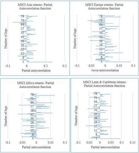
Before doing volatility forecasts, the financial time series are examined to find out whether the series is stationary. Specifically, an examination of the correlogram graphs of the series is conducted (Appendix Figure A1 and Appendix Figure A2). If the series exhibit some drift with no discernible mean, then the graph is nonstationary. Stationary time series are those that have a constant mean and variance across time. Additionally, the series’ autocorrelation function (ACF) is investigated. A delayed decay of the ACF is another inference of nonstationary (Wooldridge, 2016). Appendix Figure 1 illustrates ACF that is not progressively decaying; all series are stationary. Besides, each of the 12 augmented Dickey–Fuller (ADF) test results (Appendix Table A1) rejects the null hypothesis (H0: Market return has a unit root) at a 1% significance level. In other words, the financial time series is stationary. As GARCH and its extended families require the input data to be free from the unit root issue (Wooldridge, 2016), the correlogram and ADF findings indicate that the MSCI returns series to fulfil this criterion.

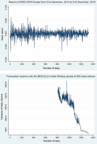
Figure 1. One step forward volatility forecasts of MSCI EFM Europe index.

A structural break is an unanticipated movement in the parameters of econometric models over the sample period, which may result in large prediction errors and model instability (Antoch et al., 2019). Thus, in addition to the stationary assessments, the tests for structural breaks in MSCI returns series (Appendix Table A2) are performed. The test set is as follows. Heteroscedasticity and autocorrelation consistent (HAC) covariances are used in the test statistics. This test configuration provides for a range of error distributions across breaks. By design, the procedure allows for a maximum of five breaks, utilizes a 15% trimming percentage, and performs sequential testing at the 0.05 significance level. Additionally, it enables error heterogeneity by allowing error distributions to vary across breaks. The test results indicate that there are no structural breaks in the return series.

The predicting performances of the HV model and the BEKK model are assessed based on the R-squared metric, mean absolute error (MAE), mean absolute percentage error (MAPE), Thiel’s inequality coefficient U1 and U2 (Theil U1 and Theil U2).

4.1. The naïve or historical variance (HV) model

The variance of the return vectors $r_t={\left(r_t^{Asia},r_t^{Europe},r_t^{Africa},r_t^{Latin\mathrm{\&}\mathrm{C}\mathrm{a}\mathrm{r}\mathrm{i}\mathrm{b}\mathrm{b}\mathrm{e}\mathrm{a}\mathrm{n}}\right)}^{\prime }={\left(r_{1,t},r_{2,t},r_{3,t},r_{4,t}\right)}^{\prime }$ is estimated using a rolling sample of 805 observations. As a result, the projections of the variance matrix for the period t + 1 are just the variance matrix for the previous 805 trading days. Pagan and Schwert (1990)’s auxiliary regression technique is used to assess forecasting ability. The realised volatility, measured by the squared returns, is regressed on a constant and the projected volatility, presuming zero mean returns for all periods (see, Table 1). This auxiliary regression model takes the following form:

$r_{i,t}^2=\alpha +\beta {\hat{\sigma }}_{i,t}^2+{\epsilon }_t$ where t = 1 … T and i = 1,2,3,4 (6)

Where:

$r_{i,t}^2$ denotes the squared rates of return of the ith MSCI index

${\hat{\sigma }}_{i,t}^2$ are the variance forecasts of the return distribution of the ith MSCI index at time t

They are the diagonal components of the rolling sample in the multivariate analysis. In Equation 6, the intercept ought to be near 0 and the slope ought to be close to 1. The t-statistics of the coefficients for $\alpha =0$ and $\beta =0$ are measures of auxiliary regression bias, whereas R-squared is a measure of overall predicting efficiency. The findings of the supplementary regressions are summarized in Table 3. The predicting performance is evaluated, based on R-squared metric, MAE, MAPE, Theil U1, and Theil U2. In terms of the R-squared metric, the projected performance is underwhelming. Africa has the lowest R-squared and the least amount of bias. Due to the poor assessment outcomes for variance estimates, any portfolio based on those projections would be unlikely to beat the benchmark, i.e. the MSCI EFM (World) index. Besides, R-squared values are less than 0.5, indicating that EFM market movements are difficult to forecast. However, the independent variables are statistically significant, which means that when the independent variable is altered by one unit, significant coefficients still indicate the mean change in the dependent variable. Other statistics provide a more detailed predicting evaluation. MAPE scores range between 53 and 55, indicating that the predicted distance from the true value is between 53% and 55% of the true value. Because Montaño Moreno et al. (2013) conclude that forecasting models with MAPE values greater than 50 are unreliable, the predicting performance of historical variance models is not quite satisfactory. Theil U1 is a prediction accuracy metric, whereas Theil U2 is a forecast quality metric. Findings in Table 3 show that while Theil U1 is within the permissible range of 0 to 1, Theil U2 is more than 1, suggesting that the forecasts under consideration are similar to those provided by the naive technique.

Table 3. The predicting performance of the historical variance (HV) model

	Asia return	Europe return	Africa return	Latin & Caribbean return
Asia variance	1.008***
	(3.770)
Europe variance		0.578**
		(2.040)
Africa variance			0.486
			(1.240)
Latin & Caribbean variance				0.809***
				(2.671)
Constant	0.000	0.000	0.000	0.000
	(0.320)	(1.543)	(1.321)	(1.072)
R-squared	0.011	0.003	0.001	0.005
AIC	−14.619	−13.107	−12.281	−12.646
SBC	−14.611	−13.099	−12.273	−12.638
The Ljung–Box Q-test (H0: No serial correlation in the error term)
Q1(4)	48.832***	146.432***	94.145***	39.171***
Q1(8)	72.053***	167.165***	102.332***	44.408***
Q2(4)	7.816	136.170	115.276***	0.622***
Q2(8)	8.429	136.530	115.790***	0.717***
ARCH effect (H0: No heteroscedastic ARCH effect)
F-Statistics	1.736	134.660***	116.078***	0.387
Probability	0.188	0.000	0.000	0.534
Predicting evaluation metrics:
MAE	0.007	0.008	0.010	0.009
MAPE	57.605	53.136	54.210	55.081
Theil U1	0.613	0.651	0.614	0.637
Theil U2	1.032	1.089	1.043	1.053

Notes: MAE = Mean absolute error, MAPE = mean absolute percentage error, Theil U1, and Theil U2 = Thiel’s inequality coefficient U1 and U2. The Q-statistics are determined for two distinct values: standardized residuals (Q1) and squared standardized residuals (Q2). This table includes the results of the following regressions: $r_{i,t}^2=\alpha +\beta {\hat{\sigma }}_{i,t}^2+{\epsilon }_t$ where $r_{i,t}^2$ denotes the squared returns of the ith MSCI index and ${\hat{\sigma }}_{i,t}^2$ are variance predictions derived using a rolling sample of the first 805 observations. The sample period runs from 1 January 2018 to 31 December 2019. T-values are in parentheses. *, **, and *** denote the significance level of 10%, 5%, and 1%, respectively.

Moreover, because the residual of the predicting model should be white noise, a diagnostic test in the form of the Ljung–Box Q-test is performed under the null hypothesis (H0: No serial correlation in the error term). The Q-statistics are determined for two distinct values: standardized residuals (Q1) and squared standardized residuals (Q2) (with special consideration on the fourth and eighth lags, which are indicated by Tse (1998)). The Q1-statistics in models of all returns are significant at the 1% level. The Q2-statistics in the model of Africa return and the model of Latin & Caribbean return are significant at the 1% level. Thus, there is insufficient evidence to invalidate the null hypothesis that all models lack serial correlation in their error component. On the other hand, the F-statistic reveals that the models (Europe return and Africa return) are not devoid of heteroscedastic ARCH effects.

4.2. The BEKK-GARCH model

Engle and Kroner (1995) propose the BEKK(p,q) model as a particular case of a vector autoregressive conditional heteroscedasticity (VARCH) model. Let $r_t$ be the N-dimensional vector of returns at time t, and a multivariate normal distribution is assumed.

(7) ${r_t}_{}N\left(\mu ,H_t\right)$(7)

Where: μ is a constant mean vector and $H_t$ is parameterized by the conditional covariance matrix structure shown below:

(8) $H_t=A_0{A}_0^{\prime }+\sum _{i=1}^p{A}_i({\epsilon }_{t-i}{\epsilon }_{t-i}^{\prime })A_i^{\prime }+\sum _{i=1}^q{B}_i{H}_{t-i}{B}_i^{\prime }$(8)

The existence of paired transposed matrices indicates a less broad parameterization than the VARCH model (where vech $H_t$ is parameterized) but enables easier maximum likelihood (ML) estimation. Since the coefficient matrices $A_0$, $A_i$, and $B_i$ exist in pairs, the conditional covariance matrix $H_t$ is non-negative-definite. The BEKK (2,2) model is selected for the returns of the four MSCI indexes using the AIC criteria. Table 4 displays the AIC and BIC for various model orderings. Employing a rolling 805 trading days, this study provides a forecast for the volatility of the returns of the MSCI EFM Asia, MSCI EFM Europe, MSCI EFM Africa, and MSCI EFM Latin America and Caribbean indexes for the out-of-sample period, from 1 January 2018 to 31 December 2019 (522 trading days).

Table 4. AIC and BIC for different orders of the BEKK model

		AIC	BIC
BEKK(1.1)		−16.590	−16.410*
BEKK(2,1)		−16.558	−16.311
BEKK(2,2)		−16.633*	−16.317
BEKK(3,2)		−16.606	−16.221

Note: The star (*) means the lowest value.

Figure 1 depicts the returns and one-step ahead estimates of the variance of the MSCI EFM Europe index, derived from the second diagonal element of the predicted variance Matrix $\left({\hat{H}}_{t+1}\right)$. Equation 8(8) $H_t=A_0{A}_0^{\prime }+\sum _{i=1}^p{A}_i({\epsilon }_{t-i}{\epsilon }_{t-i}^{\prime })A_i^{\prime }+\sum _{i=1}^q{B}_i{H}_{t-i}{B}_i^{\prime }$(8) yields the predicted variance matrix by utilizing the ML estimations for the BEKK model coefficients. To assess the predictive capabilities of the BEKK model, this study estimates auxiliary regressions (Equation 6) using the diagonal elements of ${\hat{H}}_{t+1}$ as regressors, and the results are reported in Table 5.

Table 5. The forecasting performance of the BEKK model

	Asia return	Europe return	Africa return	Latin & Caribbean return
Asia variance	1.869**
	(2.414)
Europe variance		1.350***
		(3.821)
Africa variance			3.481***
			(5.352)
Latin & Caribbean variance				1.071***
				(2.664)
Constant	0.000	0.000*	−0.001***	0.000
	(1.032)	(1.771)	(4.192)	(0.582)
R-squared	0.008	0.020	0.059	0.011
AIC	−14.990	−14.942	−13.819	−13.690
SBC	−14.950	−14.925	−13.778	−13.649
The Ljung–Box Q-test (H0: No serial correlation in the error term)
Q1(4)	15.444	5.2966	22.424	11.658
Q1(8)	31.830	10.495	36.417	21.903
Q2(4)	20.399	1.3125	1.8817	11.296
Q2(8)	26.057	3.0544	2.1319	15.576
ARCH effect (H0: No heteroscedastic ARCH effect)
F-Statistics	1.464	0.002	0.066	1.693
Probability	0.227	0.964	0.798	0.194
Forecasting evaluation metrics:
MAE	0.003	0.002	0.001	0.002
MAPE	49.545	42.824	39.509	43.151
Theil U1	0.660	0.669	0.644	0.552
Theil U2	0.808	0.744	0.721	0.789

Notes: MAE = Mean absolute error, MAPE = mean absolute percentage error, Theil U1, and Theil U2 = Thiel’s inequality coefficient U1 and U2. The Q-statistics are determined for two distinct values: standardized residuals (Q1) and squared standardized residuals (Q2). This table includes the results of the following regressions: $r_{i,t}^2=\alpha +\beta {\hat{\sigma }}_{i,t}^2+{\epsilon }_t$ where $r_{i,t}^2$ denotes the squared returns of the ith MSCI index and ${\hat{\sigma }}_{i,t}^2$ are variance forecasts. They are the diagonal components of the rolling sample in the multivariate analysis (BEKK-GARCH). T-values are in parentheses. *, **, and *** denote the significance level of 10%, 5%, and 1%, respectively.

The findings in Tables 3 and 5 are compared to demonstrate that multivariate time series models outperform the naive model. Specifically, the Q1-statistics and Q2-statistics are not statistically significant in Table 5. Thus, there is sufficient evidence to conclude that the error component of models does not exhibit serial correlation. Moreover, the F-statistic reveals that the models are devoid of heteroscedastic ARCH effects. In terms of goodness-of-fit statistics, R-squared values have improved for models of Europe, Africa, and Latin & the Caribbean. Table 5 also shows that the AIC and SBC metrics are reduced, indicating that the models in Table 5 fit the data better than those in Table 3. More importantly, diagonal components of the rolling sample in multivariate analysis (BEKK-GARCH) increase forecasting performance more than variance predictions produced from a rolling sample in the historical variance model. In terms of forecasting performance evaluation measures, all models in Table 5 have MAPE values less than 50, which Montaño Moreno et al. (2013) validate as acceptable for model forecasting performance. The values of Theil U1 are confined to the range 0 to 1. Theil U2 values are less than 1, suggesting a higher degree of predicting accuracy than the naive technique. All statistics suggest the usage of a multivariate time series model like BEKK-GARCH enhances the index volatility forecasts. Pojarliev and Polasek (2001), Ardia et al. (2017), and Ouatik El-Alaoui et al. (2018) establish that multivariate time series predictions enhance the estimate of a portfolio’s value at risk. The following section illustrates how improved variance forecasts enhance portfolio efficiency by relying on such projections.

5. Portfolio creation

Investors favour portfolios with greater mean returns and reduced risk (as assessed by standard deviation), and they will tolerate more risk in exchange for better returns. This implies that all investors should have portfolios that are on the mean-variance frontier (Allen et al., 2019; Grinold & Kahn, 2000). Each frontier portfolio return may be built by combining the market portfolio and the risk-free rate of interest. The ratio of these two funds is determined by market participants’ utility functions. If an investor is highly cautious, the individual will simply engage in the money market to obtain a risk-free rate.

The w is the vector that denotes the weights of N assets, the μ is the vector that represents the expected returns of the N assets, and H means the variance matrix of returns. The portfolio variance is defined as by ${\sigma }_p^2=w{ }^{\mathrm{\prime }}Hw$, and the portfolio return is provided by ${\mu }_p=w{ }^{\mathrm{\prime }}\mu$. Campbell et al. (1998) indicate that in the missing of a risk-free asset, the optimisation issue of a mean-variance portfolio is presented as follows. Min $w{ }^{\mathrm{\prime }}Hw$ is subject to ${\mu }_p=w{ }^{\mathrm{\prime }}\mu$ and $w{ }^{\mathrm{\prime }}t=1$ where t is a vector of ones. The solution to this optimization issue is known as the μ -fixed minimum variance (MV) portfolio because ${\mu }_p$ is set like a target:

(9) $w_p=g+h{\mu }_p$(9)

Where: $w_p$ is the weight of the MV portfolio p. The objective ${\mu }_p$ represents a predetermined portfolio return, while $g$ and h are (N × 1) vectors that are defined as follows:

(10) $g=\frac{1}{D}\left[B\left(H^{-1}t\right)-A\left(H^{-1}\mu \right)\right]$(10)

Where:$g$ is the (N × 1) vector

$B=\mu { }^{\mathrm{\prime }}{H}^{-1}\mu$

$A=t{ }^{\mathrm{\prime }}{H}^{-1}\mu$

$H^{-1}$ is the inverse variance matrix of $H_t$ which is calculated using Equation 8(8) $H_t=A_0{A}_0^{\prime }+\sum _{i=1}^p{A}_i({\epsilon }_{t-i}{\epsilon }_{t-i}^{\prime })A_i^{\prime }+\sum _{i=1}^q{B}_i{H}_{t-i}{B}_i^{\prime }$(8) .

$C=t{ }^{\mathrm{\prime }}{H}^{-1}t$

$D=BC-A^2$

(11) $h=\frac{1}{D}\left[C\left(H^{-1}\mu \right)-A\left(H^{-1}t\right)\right]$(11)

Where:$h$ is the (N × 1) vector

$B=\mu { }^{\mathrm{\prime }}{H}^{-1}\mu$

$A=t{ }^{\mathrm{\prime }}{H}^{-1}\mu$

$C=t{ }^{\mathrm{\prime }}{H}^{-1}t$

$D=BC-A^2$

$H^{-1}$ is the inverse variance matrix of $H_t$ which is calculated using Equation 8(8) $H_t=A_0{A}_0^{\prime }+\sum _{i=1}^p{A}_i({\epsilon }_{t-i}{\epsilon }_{t-i}^{\prime })A_i^{\prime }+\sum _{i=1}^q{B}_i{H}_{t-i}{B}_i^{\prime }$(8) .

If the vector denoting the weights of N assets is generated using a simpler approach, the portfolio is termed the global minimum-variance portfolio whose formula is as below:

(12) $W_{GMV}=\frac{1}{C}{H}^{-1}t$(12)

Where: $W_{GMV}$ is the weight vector of the global minimum-variance portfolio (GMV)

$C=t{ }^{\mathrm{\prime }}{H}^{-1}t$

$H^{-1}$ is the inverse variance matrix of $H_t$ which is calculated using Equation 8(8) $H_t=A_0{A}_0^{\prime }+\sum _{i=1}^p{A}_i({\epsilon }_{t-i}{\epsilon }_{t-i}^{\prime })A_i^{\prime }+\sum _{i=1}^q{B}_i{H}_{t-i}{B}_i^{\prime }$(8) .

5.1. The naive or historical variance (HV) portfolio

This study constructs the weights for the HV portfolio from the GMV calculation in Equation 12(12) $W_{GMV}=\frac{1}{C}{H}^{-1}t$(12) , employing the moving average projections of the variance matrix in section 4.1. This is because the portfolio weights are solely determined by the precision matrix $H^{-1}$ (or inverse variance matrix).

5.2. The global minimum-variance (GMV) portfolio

Rather than the simple rolling average, the one-step forward projections of the variance matrix of vectors of returns of the MSCI EFM Asia, MSCI EFM Europe, MSCI EFM Africa, and MSCI EFM Latin America and Caribbean indexes with the BEKK (2,2) model from section 4.2 are used to approximate the weights vector of global-minimum variance (GMV) portfolio for the out-of-sample period. To prevent short positions, certain portfolio weights are required to be non-negative (w ≥ 0).

5.3. The μ-fixed minimum variance (MV) portfolio

This research examines whether more forecast information may boost portfolio performance. As a result, rather than only employing the accuracy matrix, this study uses the predicted returns in the portfolio decision issue.

Equation 9(9) $w_p=g+h{\mu }_p$(9) is used to determine the weights of portfolio 3 (MV portfolio). The variance matrix H, the vector of expected asset returns $\mu$, and the intended portfolio return (${\mu }_p$) are all needed inputs. The BEKK(2,2) model projects the variance matrix and return vectors. The 3.161% per year or 0.01% every trading day is picked as the portfolio return (${\mu }_p$).

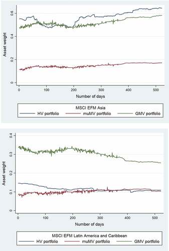
Figure 2 depicts the weights of the three portfolios for the MSCI EFM Asia and MSCI EFM Latin America and Caribbean indexes throughout the out-of-sample period. The weights for the Europe index are suppressed since all asset weights total 100%. The further prediction of the return vector ${\mu }_{t+1}$ means that the MV portfolio has more consistent weights than the GMV portfolio. Using the historical average as a projection for the HV portfolio’s variance matrix results in weights that are more consistent over time than other portfolio weights.

Figure 2. Optimal portfolio weights for the MSCI EFM Asia (Upper Panel) and the MSCI EFM Latin America and Caribbean (Lower Panel): The historical variance (HV), the μ-fixed minimum variance (MV), and the GMV for the period 1 January 2018 to 31 December 2019.

5.4. The market timing portfolio

The market-timing approach is focused on projected excess return and an asset shifting criterion. Professional investors engage in the market or a risk-free asset based on an analysis of the benchmark’s excess returns: if the gains are positive, they participate in the market; if the gains are negative, they move to cash. Cochrane (1999) and Baur et al. (2020) indicate that a market timing method (built on a regression analysis of dividend price ratio returns) produces a portfolio return with an improved Sharpe ratio. Authors demonstrate how a market timing technique may nearly double a portfolio’s average returns over 5 years.

5.4.1. Market timing rule based on volatility forecasts

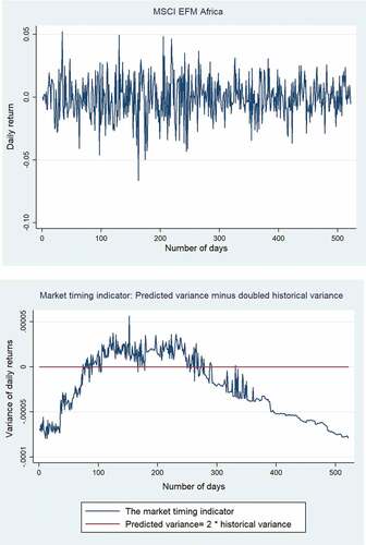
The market timing rule for returns is set up, based on volatility estimates. Because of the possible trade-off between risk and reward, assets with more volatility have greater returns. As a result, the following rigorous market timing rule is suggested. An investor engages in the market if the predicted volatility is two times higher than the historical volatility; alternatively, the individual participates in a risk-free asset. It should be noted that shifting to a risk-free asset reduces portfolio variance.

Figure 3 lower panel depicts the market timing indication for the Africa area. If the predicted (Africa) variation is double the previous variance, the investor puts money in the Africa index. The horizontal line denotes the days when the predicted (Africa) variance is twice and equals the historical variance (the market timing indicator is equal to zero). When the indicator crosses the horizontal line, an individual invests in the Africa index, and conversely. Likewise, market-timing indicators are established for Europe, Asia, Latin America, and the Caribbean.

Figure 3. MSCI EFM Africa returns and the market timing indicator.

The portfolio return for every period becomes a possible combination of the risk-free rate and territorial index returns. It should be noted that this method does not guarantee that chosen returns are always higher than the risk-free rate. If strong volatility periods create returns that are lower than the risk-free rate, an average portfolio return (in one or more phases) may fall underneath the risk-free rate. If the indicator is positive, the corresponding MSCI index is picked; alternatively, cash is selected. In the multivariate scenario, an individual invests the index using the same weights as in the GMV portfolio. For a risk-free rate, the assumed rate of interest is 5% per year; else, the investor may opt to engage in the bond market.

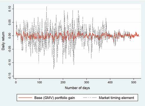
Figure 4 depicts the cumulative benefit of the market timing approach. The total portfolio returns are divided into two parts: 1) the base portfolio gain resulting from the GMV portfolio’s returns, and 2) the added gain resulting from the general market timing criterion. Positive returns outnumber negative returns in this MT element. In the autumn of 2019, the additional gain became consistent and positive. This demonstrates that an investor may use the trade-off between risk and return in the regional portfolio to determine the appropriate asset allocation at a given moment. The plateaus in the MT element represent times when the GMV portfolio—which is depicted as a straight line—dictates the return of the MT portfolio. The non-plateau period includes any time when investors from at least a single area choose not to participate in the regional index.

Figure 4. Elements of the market timing portfolio in aggregate.

6. Portfolio scenario comparison

The portfolio result is evaluated to the MSCI EFM (World) index for the out-of-sample timespan (1 January 2018–31 December 2019) that uses the specific objectives: The yearly mean return (in percent), the yearly standard deviation (in percent), the cumulative return for 2 years and year to date (in percent), the Sharpe ratio, and the success rate.

The Sharpe ratio $S_p$ is specified as the expected excess return of a portfolio (p) divided by the risk of that portfolio, in which the risk-free rate is considered to be 5% annually.

(13) $S_p=\frac{E\left[r_p-r_{risk-free}\right]}{{\sigma }_p}$(13)

Where: $S_p$: the Sharpe ratio of the portfolio p

$r_p$: the rate of return of the portfolio p

$r_{risk-free}$: the risk-free rate of return of the market.

$E\left[r_p-r_{risk-free}\right]$: the expected rate of return of the portfolio p

${\sigma }_p$: the standard deviation of the portfolio p’s rates of return.

The Sharpe ratio represents the correlation between the provided asset allocation and the market portfolio (Harvey & Zhou, 1990). The success rate is measured as the fraction of monthly occasions when the portfolio returns outperform the benchmark (MSCI EFM index) returns.

Table 6 highlights the portfolio evaluations based on the five factors. The HV portfolio outperforms the benchmark, whereas the GMV portfolio exceeds both the HV portfolio and the benchmark based on a one-step forward projection of the variance matrix in the BEKK (2,2) model. The GMV portfolio has higher mean returns and a lower standard deviation, for example. The MV portfolio trumps all other portfolios in terms of returns. The year-to-date record of the MV portfolio is lower than that of the MT portfolio (year-to-date cumulative returns begin on 1 January 2019), but it has considerably more steady portfolio weights, which subsequently result in lower transaction fees. Portfolio four (the MT portfolio) is the overall second best portfolio based on the market timing approach, but it exceeds other portfolios in 2019.

Table 6. Performance measures of portfolios versus the benchmark portfolio (MSCI EFM (World) index). Cumulative returns for 2 years (from 1 January 2018 until 31 December 2019) and year-to-date returns for the year 2019

	HV portfolio	GMV portfolio	MV portfolio	MT portfolio	Benchmark
Mean returns	1.210%	1.640%	3.475%	1.774%	−1.049%
Standard deviation	13.006%	12.982%	14.913%	14.202%	13.510%
Cumulative returns (2 years)	2.436%	3.308%	7.070%	3.580%	−2.087%
Year-to-date return	19.555%	19.702%	23.807%	24.153%	16.160%
Sharpe ratio	−0.291	−0.259	−0.102	−0.227	−0.448
Success rate	51.533%	50.575%	51.916%	51.724%

Notes: This table provides statistics for five portfolio criteria: mean returns, the standard deviation, cumulative returns (2 years), year-to-date return (2019), Sharpe ratio, and success rate. The portfolios under consideration are the historical variance (HV) portfolio, the global-minimum variance (GMV) portfolio, the μ-fixed minimum variance (MV) portfolio, the market timing (MT) portfolio, and the MSCI EFM (World) index or the benchmark portfolio.

Yearly, the MV portfolio outperforms the benchmark by about 4.5 percentage points and is behind just the MT portfolio in the year-to-date comparison. The Sharpe ratio is likewise the highest for the MV portfolio, which is attributable to higher portfolio returns. The success percentage for all portfolios is modest and marginally higher than 50% for the market timing portfolio. This could indicate that the greater yields from the MV are focused on in a few intervals.

7. Conclusion

The role of frontier markets or pre-emerging markets in global stock portfolio diversification is less unexplored, and studying their diversification potential can provide important implications to international investors. Using daily returns from 1 January 2014 to 31 December 2019, this study examines how optimal holdings for EFM markets in four global regions differ from the benchmark weights. Specifically, this study provides a multivariate time series model which is used to enhance stock index volatility forecasts. It demonstrates how the returns of the MSCI EFM Asia, MSCI EFM Europe, MSCI EFM Africa, and MSCI EFM Latin America and Caribbean indexes may be used to enhance portfolio efficiency in a three-dimensional portfolio model. As a reference, the MSCI EFM (World) index is utilised. Moreover, a market-timing portfolio is developed based on volatility projections. According to the market timing strategy, an investor only invests in the stock index if the predicted volatility is twice as high as the historical volatility.

The empirical investigation gives the following research findings. First, in comparison to the predicting performance of the historical variance model, the forecasting performance of the BEKK-GARCH model is free from serial correlation in the error term and heteroscedastic ARCH effects. Goodness-of-fit statistics (AIC and SBC) are also lower. Besides, the forecasting evaluation metrics are enhanced in the performance of the BEKK-GARCH model. Second, the portfolio analysis proves that the market timing (MT) portfolio works effectively, only being outperformed by the μ-fixed minimum variance (MV) portfolio overall. For the previous 2 years, it has lower cumulative returns and lower standard deviation than those of the MV portfolio. Finally, the MT portfolio becomes the best in terms of consistent and positive returns in 2019 and beyond.

The findings of this article have important implications for academicians and investors looking to diversify their portfolios into EFM markets. There are three recommendations withdrawn from the study findings for academicians. First, the forecasting performances of two volatility models in terms of predicting accuracy (R-squared metric, MAE, MAPE, Theil U1, and Theil U2) provide a significant recommendation for research scholars. Specifically, the academic researcher can obtain better stock index return volatility forecasts by using the naive or historical variance model than by employing the multivariate time series model. Second, research scholars can effectively obtain volatility forecasts from multivariate time series models and translate the results into greater portfolio returns via quantitative investment methods in their study, if the proper mix of volatility modelling and portfolio strategy is identified. Finally, the impressive performance of the portfolio employing the market-timing strategy in this study gives recommendations for academicians that there are strategic approaches that may successfully utilise the trade-off between risk and returns and are worth considering in addition to standard ways such as the minimum-variance strategy. Furthermore, there are two recommendations withdrawn from the study findings for investors. First, although different market timing strategies are available for practice, their effectiveness should be proven. Hence, the first recommendation for investors is that studies on market timing strategies might become increasingly relevant in the future, especially for institutional investors (for example, fund managers) seeking to exceed benchmarks in a somewhat more technical manner. Also, different investment strategies provide different investment outcomes (for example, portfolio returns and portfolio variance). The second recommendation for investors is that their choice of investment strategies can be one or a mix of different approaches that should depend on their investment priorities (for example, risk minimization, profit maximization, or a specific investment objective).

The research provides some recommendations for future research. If the sample data contains structural breaks, a proxy for structural change should be added to the multivariate time series model. Second, this study employs BEKK-GARCH as the multivariate time series model of choice to enhance stock index volatility forecasts. A future analysis might broaden the technique selections, and testing alternative datasets and frequencies could aid in expanding our understanding of volatility forecasting and translating it into more prudent asset allocation.

Acknowledgements

I wish to express my gratitude to the editor and two anonymous referees for their constructive suggestions. Any remaining faults are entirely my fault. My deepest gratitude to Professor Sử Đình Thành, my academic supervisor, for his committed, whole-hearted coaching and assistance during the completion of the paper as a part of my doctoral dissertation.

Disclosure statement

No potential conflict of interest was reported by the author.

Additional information

Funding

The author received no direct funding for this research.

Notes on contributors

Tri M. Hoang

Tri M. Hoang is a Ph.D. student at the University of Economics Ho Chi Minh City (UEH) in Vietnam, working under the guidance of Prof. Su Dinh Thanh. His thesis examines the diversification of asset returns in portfolio management for investors from emerging markets. This article is based on a section of his doctoral thesis. Tri M. Hoang is also a lecturer at Vietnam’s Ho Chi Minh City University of Technology (HUTECH). Behavioral finance and markets, as well as empirical asset pricing, are among his research interests.

Appendix

Table A1. The unit root test results for the MSCI emerging and frontier market series from 1 December 2014 to 31 December 2019

	Augmented Dickey-Fuller (ADF) test
	H0: Market return has a unit root
	Intercept		Trend and Intercept		Without Trend and Intercept
	Test Statistics	Probability	Test Statistics	Probability	Test Statistics	Probability
Asia	-31.785	0.000	-31.777	0.000	-31.783	0.000
Europe	-33.224	0.000	-33.242	0.000	-33.233	0.000
Africa	-34.449	0.000	-34.438	0.000	-34.462	0.000
Latin & Caribbean	-33.205	0.000	-33.209	0.000	-33.217	0.000
World	-29.527	0.000	-29.525	0.000	-29.532	0.000

Table A2. The structural test results for the MSCI frontier market series

	Bai–Perron sequential tests of L + 1 vs. L sequentially determined breaks
	Break Test	F-statistic	Scaled F-statistic	Critical Value
	nulls vs. alternatives (*)
Asia	0 vs. 1	3.324	3.324	8.580
Europe	0 vs. 1	4.239	4.239	8.580
Africa	0 vs. 1	3.699	3.699	8.580
Latin & Caribbean	0 vs. 1	5.839	5.839	8.580

This table summarizes Bai’s (1997) and Bai and Perron’s sequential Bai and Perron (1998). There is an F-statistic, as well as an F-statistic scaled by the number of varying regressors (which is the same in this situation, as there is only one varying regressor), and a Bai–Perron critical value for the scaled statistic calculated from Bai and Perron (2003). The break test displays nulls on the left and alternatives on the right, with the number of breaks given by (*) or significance at the 0.05 level.

Figure A1. The autocorrelation function (ACF) of the MSCI index returns.

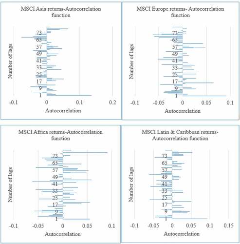
Figure A2. The partial autocorrelation function (PACF) of the MSCI index returns.

References

- Al Janabi, M. A. M. (2021). Is optimum always optimal? A revisit of the mean-variance method under nonlinear measures of dependence and non-normal liquidity constraints. Journal of Forecasting, 40(3), 387–27. https://doi.org/10.1002/for.2714
- Albeverio, S., Steblovskaya, V., & Wallbaum, K. (2013). Investment instruments with volatility target mechanism. Quantitative Finance, 13(10), 1519–1528. https://doi.org/10.1080/14697688.2013.804943
- Alexander, G. J., & Baptista, A. M. (2002). Economic implications of using a mean-VaR model for portfolio selection: A comparison with mean-variance analysis. Journal of Economic Dynamics & Control, 26(7), 1159–1193. https://doi.org/10.1016/S0165-1889(01)00041-0
- Allen, D., Lizieri, C., & Satchell, S. (2019). In defense of portfolio optimization: what if we can forecast? Financial Analysts Journal, 75(3), 20–38. https://doi.org/10.1080/0015198X.2019.1600958
- Antoch, J., Hanousek, J., Horváth, L., Hušková, M., & Wang, S. (2019). Structural breaks in panel data: Large number of panels and short length time series. Econometric Reviews, 38(7), 828–855. https://doi.org/10.1080/07474938.2018.1454378
- Ardia, D., Bolliger, G., Boudt, K., & Gagnon-Fleury, J.-P. (2017). The impact of covariance misspecification in risk-based portfolios. Annals of Operations Research, 254(1), 1–16 https://doi.org/10.1007/s10479-017-2474-7.
- Asness, C. S., Frazzini, A., & Pedersen, L. H. (2012). Leverage aversion and risk parity. Financial Analysts Journal, 68(1), 47–59. https://doi.org/10.2469/faj.v68.n1.1
- Bai, J. (1997). Estimating multiple breaks one at a time. Econometric Theory, 13(3), 315–352. https://doi.org/10.1017/S0266466600005831
- Bai, J., & Perron, P. (1998). Estimating and testing linear models with multiple structural changes. Econometrica, 66(1), 47–78. https://doi.org/10.2307/2998540
- Bai, J., & Perron, P. (2003). Critical values for multiple structural change tests. The Econometrics Journal, 6(1), 72–78. https://doi.org/10.1111/1368-423X.00102
- Baur, D. G., Dichtl, H., Drobetz, W., & Wendt, V.-S. (2020). Investing in gold – Market timing or buy-and-hold? International Review of Financial Analysis, 71 October 2020 , 101281. https://doi.org/10.1016/j.irfa.2018.11.008
- Bednarek, Z., & Patel, P. (2018). Understanding the outperformance of the minimum variance portfolio. Finance Research Letters, 24, 175–178. https://doi.org/10.1016/j.frl.2017.09.005
- Bergmann, D. R., Ferreira Savoia, J. R., Felisoni de Angelo, C., Contani, E. A. D. R., & Silva, F. L. D. (2018). Portfolio management with tail dependence. Applied Economics, 50(51), 5510–5520. https://doi.org/10.1080/00036846.2018.1487000
- Berk, J., & Demarzo, P. M. (2020). Corporate finance (5th ed.). Pearson.
- Bian, Z., Liao, Y., O’Neill, M., Shi, J., & Zhang, X. (2020). Large-scale minimum variance portfolio allocation using double regularization. Journal of Economic Dynamics & Control, 116 July 2020 , 103939. https://doi.org/10.1016/j.jedc.2020.103939
- Blume, M. E., & Friend, I. (1974). Risk, investment strategy and the long-run rates of return. The Review of Economics and Statistics, 56(3), 259–269. https://doi.org/10.2307/1923963
- Bodie, Z., Kane, A., & Marcus, A. (2018). Investments (11 ed.). McGraw-Hill Education.
- Bodnar, T., Parolya, N., & Schmid, W. (2018). Estimation of the global minimum variance portfolio in high dimensions. European Journal of Operational Research, 266(1), 371–390. https://doi.org/10.1016/j.ejor.2017.09.028
- Bollerslev, T. (1986). Generalized autoregressive conditional heteroskedasticity. Journal of Econometrics, 31(3), 307–327. https://doi.org/10.1016/0304-4076(86)90063-1
- Bollerslev, T., Engle, R. F., & Wooldridge, J. M. (1988). A capital asset pricing model with time-varying covariances. Journal of Political Economy, 96(1), 116–131. https://doi.org/10.1086/261527
- Busse, J. A. (1999). Volatility timing in mutual funds: evidence from daily returns. The Review of Financial Studies, 12(5), 1009–1041. https://doi.org/10.1093/rfs/12.5.1009
- Campbell, J. Y., Lo, A. W., MacKinlay, A. C., & Whitelaw, R. F. (1998). The econometrics of financial markets. Macroeconomic Dynamics, 2(4), 559–562. https://doi.org/10.1017/S1365100598009092
- Chan, L. K. C., Karceski, J., & Lakonishok, J. (1999). On portfolio optimization: forecasting covariances and choosing the risk model. The Review of Financial Studies, 12(5), 937–974. https://doi.org/10.1093/rfs/12.5.937
- Choueifaty, Y., & Coignard, Y. (2008). Toward maximum diversification. The Journal of Portfolio Management, 35(1), 40–51. https://doi.org/10.3905/JPM.2008.35.1.40
- Clarke, R. G., de Silva, H., & Thorley, S. (2006). Minimum-variance portfolios in the U.S. equity market. The Journal of Portfolio Management, 33(1), 10–24. https://doi.org/10.3905/jpm.2006.661366
- Clarke, R., de Silva, H., & Thorley, S. (2011). Minimum-variance portfolio composition. The Journal of Portfolio Management, 37(2), 31–45. https://doi.org/10.3905/jpm.2011.37.2.031
- Cochrane, J. H. (1999). Portfolio advice for a multifactor world. Economic Perspectives 23 QIII 59–78 . https://doi.org/10.3386/w7170 Federal Reserve Bank of Chicago
- Costa, G., & Kwon, R. H. (2019). Risk parity portfolio optimization under a Markov regime-switching framework. Quantitative Finance, 19(3), 453–471. https://doi.org/10.1080/14697688.2018.1486036
- Cronqvist, H., & Siegel, S. (2014). The genetics of investment biases. Journal of Financial Economics, 113(2), 215–234. https://doi.org/10.1016/j.jfineco.2014.04.004
- Cumova, D., & Nawrocki, D. (2014). Portfolio optimization in an upside potential and downside risk framework. Journal of Economics and Business, 71 January–February 2014 , 68–89. https://doi.org/10.1016/j.jeconbus.2013.08.001
- De Jong, M., & Fabozzi, F. J. (2021). From ad hoc bond-risk measures to variance–covariance forecasts. The Journal of Fixed Income, 30(4), 6–16. https://doi.org/10.3905/jfi.2021.1.105
- DeMiguel, V., Garlappi, L., & Uppal, R. (2009). Optimal versus naive diversification: how inefficient is the 1/n portfolio strategy? The Review of Financial Studies, 22(5), 1915–1953 https://doi.org/10.1093/rfs/hhm075.
- Disatnik, D., & Katz, S. (2012). Portfolio optimization using a block structure for the covariance matrix. Journal of Business Finance & Accounting, 39(5–6), 806–843. https://doi.org/10.1111/j.1468-5957.2012.02279.x
- Doan, B., Papageorgiou, N., Reeves, J. J., & Sherris, M. (2018). Portfolio management with targeted constant market volatility. Insurance, Mathematics & Economics, 83 November 2018 , 134–147. https://doi.org/10.1016/j.insmatheco.2018.09.010
- Dos Santos, S. F., & Brandi, H. S. (2017). Selecting portfolios for composite indexes: Application of modern portfolio theory to competitiveness. Clean Technologies and Environmental Policy, 19(10), 2443–2453. https://doi.org/10.1007/s10098-017-1441-y
- Elton, E. J., & Gruber, M. J. (1973). Estimating the dependence structure of share prices —implications for portfolio selection. The Journal of Finance, 28(5), 1203–1232. https://doi.org/10.1111/j.1540-6261.1973.tb01451.x
- Elton, E. J., Gruber, M. J., Padberg, M. W., Marczyńska-Wolańska, H., & Bocheńska, E. (1976). Simple criteria for optimal portfolio selection. Polski tygodnik lekarski (Warsaw, Poland: 1960), 31(5), 1341–1357 doi:10.1111/j.1540-6261.1976.tb03217.x .
- Engle, R. F., & Kroner, K. F. (1995). Multivariate simultaneous generalized ARCH. Econometric Theory, 11(1), 122–150. https://doi.org/10.1017/S0266466600009063
- Fabozzi, F., & Markowitz, H. (2011). The theory and practice of investment management: asset allocation, valuation, portfolio construction, and strategies, second edition (the theory and practice of investment management. John Wiley & Sons. https://doi.org/10.1002/9781118267028
- Golosnoy, V., Gribisch, B., & Seifert, M. I. (2021). Sample and realized minimum variance portfolios: Estimation, statistical inference, and tests. WIREs Computational Statistics N/A , (e1556), 1–18 . https://doi.org/10.1002/wics.1556
- Grinold, R., & Kahn, R. N. (2000). Active portfolio management: A quantitative approach for providing superior returns and controlling risk (2nd ed.). McGraw Hill Professional.
- Harvey, C. R., & Zhou, G. (1990). Bayesian inference in asset pricing tests. Journal of Financial Economics, 26(2), 221–254. https://doi.org/10.1016/0304-405X(90)90004-J
- Holthausen, R. W. (1981). Evidence on the effect of bond covenants and management compensation contracts on the choice of accounting techniques: The case of the depreciation switch-back. Journal of Accounting and Economics, 3(1), 73–109. https://doi.org/10.1016/0165-4101(81)90035-5
- Hwang, I., Xu, S., & In, F. (2018). Naive versus optimal diversification: Tail risk and performance. European Journal of Operational Research, 265(1), 372–388. https://doi.org/10.1016/j.ejor.2017.07.066
- Jagannathan, R., & Ma, T. (2003). Risk reduction in large portfolios: why imposing the wrong constraints helps. The Journal of Finance, 58(4), 1651–1683. https://doi.org/10.1111/1540-6261.00580
- Kempf, A., & Memmel, C. (2006). Estimating the global minimum variance portfolio. Schmalenbach Business Review, 58(4), 332–348. https://doi.org/10.1007/BF03396737
- King, B. F. (1966). Market and industry factors in stock price behavior. The Journal of Business, 39(1), 139–190. https://doi.org/10.1086/294847
- Ledoit, O., & Wolf, M. (2003). Improved estimation of the covariance matrix of stock returns with an application to portfolio selection. Journal of Empirical Finance, 10(5), 603–621. https://doi.org/10.1016/s0927-5398(03)00007-0
- Ledoit, O., & Wolf, M. (2004). Honey, I shrunk the sample covariance matrix. The Journal of Portfolio Management, 30(4), 110–119. https://doi.org/10.3905/jpm.2004.110
- Ledoit, O., & Wolf, M. (2017). Nonlinear shrinkage of the covariance matrix for portfolio selection: Markowitz meets goldilocks. The Review of Financial Studies, 30(12), 4349–4388. https://doi.org/10.1093/rfs/hhx052
- Ledoit, O., & Wolf, M. (2020). The power of (non-)linear shrinking: a review and guide to covariance matrix estimation. Journal of Financial Econometrics 20 01 187–218 https://doi.org/10.1093/jjfinec/nbaa007 .
- Lintner, J. (1956). Distribution of incomes of corporations among dividends, retained earnings, and taxes. The American Economic Review, 46(2), 97–113. http://www.jstor.org/stable/1910664
- Maillard, S., Roncalli, T., & Teïletche, J. (2010). The properties of equally weighted risk contribution portfolios. The Journal of Portfolio Management, 36(4), 60–70. https://doi.org/10.3905/jpm.2010.36.4.060
- Markowitz, H. (1952). Portfolio selection. The Journal of Finance, 7(1), 77–91. https://doi.org/10.1111/j.1540-6261.1952.tb01525.x
- Markowitz, H. M. (1959). Portfolio selection: efficient diversification of investments. Yale University Press. www.jstor.org/stable/j.ctt1bh4c8h
- Montaño Moreno, J. J., Palmer Pol, A., Sesé Abad, A., & Cajal Blasco, B. (2013). Using the R-MAPE index as a resistant measure of forecast accuracy. Psicothema, 25(4), 500–506 https://doi.org/10.7334/psicothema2013.23.
- MSCI. (2017). MSCI frontier market index fact sheet https://www.msci.com/documents/10199/f9354b32-04ac-4c7e-b76e-460848afe026
- MSCI. (2019). Index solutions https://www.msci.com/index-solutions
- Ouatik El-Alaoui, A., Ismath Bacha, O., Masih, M., & Asutay, M. (2018). Does low leverage minimise the impact of financial shocks? New optimisation strategies using Islamic stock screening for European portfolios. Journal of International Financial Markets, Institutions and Money, 57 November 2018 , 160–184. https://doi.org/10.1016/j.intfin.2018.07.007
- Pafka, S., & Kondor, I. (2004). Estimated correlation matrices and portfolio optimization. Physica A: Statistical Mechanics and Its Applications, 343 15 November 2004 , 623–634. https://doi.org/10.1016/j.physa.2004.05.079
- Pagan, A. R., & Schwert, G. W. (1990). Alternative models for conditional stock volatility. Journal of Econometrics, 45(1–2), 267–290 https://doi.org/10.1016/0304-4076(90)90101-X.
- Pätäri, E., Ahmed, S., John, E., Karell, V., McMillan, D., & McMillan, D. (2019). The changing role of emerging and frontier markets in global portfolio diversification. Cogent Economics & Finance, 7(1), 1–24. https://doi.org/10.1080/23322039.2019.1701910
- Pojarliev, M., & Polasek, W. (2001). Applying multivariate time series forecasts for active portfolio management. Financial Markets and Portfolio Management, 15(2), 201–211. https://doi.org/10.1007/s11408-001-0205-0
- Pojarliev, M., & Polasek, W. (2003). Portfolio construction by volatility forecasts: Does the covariance structure matter? Financial Markets and Portfolio Management, 17(1), 103–116. https://doi.org/10.1007/s11408-003-0105–6
- Rabouin, D. (2017). Foreign investors to pour nearly $1 trillion into emerging markets in 2017: IIF. Reuters https://www.reuters.com/article/us-emerging-flows-iif-idUSKBN18X1NJ
- Ross, S. A. (1976). The arbitrage theory of capital asset pricing. Journal of Economic Theory, 13(3), 341–360. https://doi.org/10.1016/0022-0531(76)90046-6
- Roy, A. D. (1952). Safety first and the holding of assets. Econometrica, 20(3), 431–449. https://doi.org/10.2307/1907413
- Sharpe, W. F. (1963). A simplified model for portfolio analysis. Management Science, 9(2), 277–293. https://doi.org/10.1287/mnsc.9.2.277
- Sharpe, W. F. (1964). Capital asset prices: a theory of market equilibrium under conditions of risk. The Journal of Finance, 19(3), 425–442. https://doi.org/10.1111/j.1540-6261.1964.tb02865.x
- Sotiroff, D. (2021). Is emerging-markets investing worth the risk? Morningstar, Inc. https://www.morningstar.com/articles/1032508/is-emerging-markets-investing-worth-the-risk
- Speidell, L. S. (2011). Frontier markets equity investing: finding the winners of the future (CFA Institute Research Foundation M2011–2 (Vol. 2011. The CFA Institute Research Foundation.
- Stein, C. (1956). Volume 1 contribution to the theory of statistics (inadmissibility of the usual estimator for the mean of a multivariate normal distribution. University of California Press. https://doi.org/10.1525/9780520313880-018
- Theron, L., van Vuuren, G., & McMillan, D. (2018). The maximum diversification investment strategy: A portfolio performance comparison. Cogent Economics & Finance, 6(1), 1–16. https://doi.org/10.1080/23322039.2018.1427533
- Treynor, J. (1965). How to rate management of investment funds. Harvard Business Review, 43(1), 63–75 https://doi.org/10.1002/9781119196679.ch10.
- Tse, Y. K. (1998). The conditional heteroscedasticity of the yen-dollar exchange rate. Journal of Applied Econometrics, 13(1), 49–55. https://doi.org/10.1002/(SICI)1099-1255(199801/02)13:1<49::AID-JAE459>3.0.CO;2-O
- Vasicek, O. A. (1973). A note on using cross-sectional information in bayesian estimation of security betas. The Journal of Finance, 28(5), 1233–1239. https://doi.org/10.2307/2978759
- Wooldridge, J. M. (2016). Introductory econometrics: A modern approach (6th ed.). South-Western Cengage Learning.
- Zakamulin, V. (2015). A test of covariance-matrix forecasting methods. The Journal of Portfolio Management, 41(3), 97–108. https://doi.org/10.3905/jpm.2015.41.3.097
- Zhu, B., & Zhang, T. (2021). Long-term wealth growth portfolio allocation under parameter uncertainty: A non-conservative robust approach. The North American Journal of Economics and Finance, 57(1), 1–24. https://doi.org/10.1016/j.najef.2021.101432