Floating versus fixed: How exchange rate regimes affect business cycles comovement between advanced and emerging economies

Abstract

This article investigates the effects of the different exchange rate regimes on business cycles comovement between advanced and emerging countries. We use the Granger Causality test (VAR model) on panel data to examine the causal relationships. Our findings show the existence of a bidirectional causal relationship between output comovement and the exchange rate regimes. We check the robustness of our results by applying Dumitrescu-Hurlin (2012) panel causality test that confirms our findings. Furthermore, the impulse response functions illustrate that business cycles comovement between advanced and emerging economies responds positively and significantly to the exchange rate regimes of these two groups of countries in the short term. However, the positive effect begins to wane before being negative from the third quarter and the fifth quarter for emerging economies and developed economies, respectively.

Keywords:

• Business cycle
• exchange rate regime
• synchronization
• emerging economies
• advanced economies

JEL:

• E32
• F44
• E42
• F15
• F31

1. Introduction

Emerging countries have steadily been increasing their role in the international economic system. The share of emerging and developing economies in world GDP reached 58.7% in 2018, compared to 30.9% in 1980.¹ From an economic point of view, they have made significant progress in several areas, represented mainly by the growth of foreign direct investments (FDI), portfolio investments, international reserves and, more generally, their shares in international trade.

Along with this significant growth in emerging economies, a lively debate has arisen on business cycles synchronization between advanced and emerging countries. Developed economies recorded a 7.5% decline in real GDP in the fourth quarter of 2008.² However, the main emerging countries, notably India and China, continued to perform well in terms of real growth. This started a relative debate on the decoupling hypothesis. Elgahry (2014) found that the latter arises from the fact that, if national economies are increasingly interconnected, this should make these economies more dependent on each other, while at the same time, emerging economies have become much larger and more autonomous.

In fact, many explanations for business cycles coupling point out that all economies have become more linked through trade and financial channels, which is likely to strengthen economic conjunctures. Supporters of the decoupling hypothesis, however, have observed that the evidence is based on the idea that, alongside the significant economic growth of emerging countries, the development of trade and financial linkages between these economies could have strengthened the relations between this group of countries to the detriment of others. Thus, their relations with advanced economies may have relatively weakened (Pesce, 2015).

Moreover, many theories of the international transmission of shocks (real shocks or shocks due to monetary policy) imply that the process of transmission critically depends on the exchange rate regime (Baxter & Stockman, 1989). One of the empirical implications of these theories is that, by keeping the sources of exogenous shocks and their stochastic processes constant, the variances and covariances of economic aggregates will depend on the exchange rate system. While some attention has been paid to the relationships between international reserves and the main determinants of business cycles synchronization (financial and trade integration), a limited number of previous studies have linked the correlation of business cycles to the different exchange rate regimes. Among the studies which have discussed this issue, we can mention that of Gerlach et al. (1988) who showed a relationship between business cycles transmission between OECD countries and exchange rate systems, fixed and floating. This study concludes that monthly variations in industrial production in these countries are more pronounced in floating exchange rate systems than in fixed exchange rate regimes. In addition, Baxter and Stockman (1989) found that the volatility of output in floating regimes is more significant than in fixed exchange rate systems. Finally, Erdem and Özmen (2015) empirically studied the effects of internal and external factors as well as exchange rate regimes on business cycles transmission. Their results suggest that emerging economies tend to experience much deeper recessions and relatively stronger expansions for almost the same length of time. The probability of expansion increases considerably with the flexibility of the exchange rate regime. Moreover, their findings strongly support a floating exchange rate regime for advanced countries and emerging countries other than East Asian countries. In contrast, Artis and Zhang (1997) have pointed out that a fixed exchange rate regime is likely to lead to the synchronization of business cycles. Hou and Knaze (2019) confirm this last finding by explaining that the correlation coefficient of business cycles is about 0.12 points higher in countries with no separate legal tenders.

Therefore, this article aims to fill this gap by testing the effects of different exchange rate regimes on the degree of business cycles comovement between emerging and advanced economies over a quarterly series from 2000 to 2016. In other words, does the nature of the exchange rate regime affect the degree of business cycles correlation between these two groups of countries? By examining the impact of exchange rate system on output comovement between advanced and emerging countries, this article engages with the aforementioned arguments, which appear to provide contradictory assessments with regards to the effect of the exchange rate regime on business cycles correlation.

We want to emphasize that the present study differs from that of Erdem and Özmen (2015) on several points. First, on the number of countries, the sample under consideration includes 35 advanced countries and 26 emerging countries, while the other includes 23 developed economies and 27 emerging economies. Secondly, from a methodological standpoint, Erdem and Özmen (2015) consider the classic business cycles defined by Mitchell, 1927), while this study estimates business cycles comovement according to the recent method developed by Abiad et al. (2013) which allows us to calculate the output comovement at any point in time, as mentioned below. Moreover, unlike Erdem and Ozmen, who adopted the Panel ARDL method, we use two techniques: Granger Causality test (VAR modeling) on panel data and the impulse responses of the business cycles correlation to the different variables. Lastly, Erdem and Özmen’s dissertation is based on quarterly data from 1960 to 2013 for advanced countries and from 1980 for most emerging countries. For Eastern European countries, the authors do not have data until after the mid-1990s. The present study, however, covers a quarterly series from 2000 to 2016 for all advanced and emerging countries.

We have chosen this period (2000Q1–2016Q4) for three reasons. First, in the early 2000s, new macroeconomic considerations emerged about the role played by international capital flows and domestic financial systems in determining the performance of exchange rate regimes (Reinhart et al., 2003). In this regard, it has been observed that Portfolio Investment (IP) openness for emerging countries has more than doubled in five years, from 11% in 2002 to 27% in 2007. As for the Foreign Direct Investment (FDI) openness for the same group of countries, it has recorded a significant growth of almost 90%, from 2.56% in 2002 to 4.9%—its peak—in 2008 (Elgahry & Baher, 2014). This shows the rapid growth of the financial integration of these economies over the past decade.

This period is also significant in so far as it saw the official introduction of the euro as legal tender at the beginning of 2002, which has a significant impact on the European business cycles synchronization. Campos et al. (2019) found that business cycles correlation between European countries increased by 50% after the changeover to the euro and that this growth was greater in euro zone countries.

Finally, according to the IMF, three episodes of financial crises were observed in advanced countries during this period (2000–2016): The stock market crash in 2000), the global financial crisis of 2008) and the debt crisis in the euro area in 2010), during which output reached its lowest level. Thus, testing the degree of business cycles comovement between the advanced group and the emerging group during these crises periods as well as distinguishing it according to the different exchange rate regimes appears relevant.

Therefore, this paper aims to provide empirical elements to address the problem statement aforementioned. After discussing how the literature approaches the different exchange rate regimes and business cycles comovement, we will expose the methodology and the empirical model. The causal relationships are examined by the Granger Causality test (VAR modeling) on panel data. Then, we support our findings by estimating the impulse response. Finally, we conclude.

2. Exchange rate regimes and business cycles comovement: literature approach

The study of business cycles and their international transmission is one of the oldest topics of economics. The first detailed statistical analyses of business cycles were undertaken in the 1920s by the National Bureau of Economic Research (NBRE) under the direction of Wesley Clair Mitchell. The latter studied the international correlation of business cycles in his book “Business Cycles: The Problem and Its Setting (1927)”. He concluded that business cycles are positively correlated between countries, especially advanced countries and more particularly those with well-developed financial markets. He also found that business cycles were increasingly correlated between countries over time and attributed it to the growth of international financial linkages.

Findlay, 1974) developed the logic of the insulation value of floating exchange rates in his famous textbook “International Economics”. He is best known for his work comparing a fixed exchange rate and a floating exchange rate system of small open economies with perfect capital mobility. Mundell also discussed a two-country model in an appendix to Chapter 18. He showed that at a fixed exchange rate, monetary shocks lead to a positive synchronization of the business cycle while the effect of real shocks is theoretically ambiguous. In contrast, under a floating exchange rate regime, real shocks are associated with positive contagions as well as cyclical transmissions for large countries. It explicitly states that it cannot therefore be said that a country is automatically immune by its flexible exchange rate to fluctuations in the business cycle from outside. His argument is that a positive domestic real shock increases the domestic interest rate, thus attracting foreign capital and appreciating the exchange rate. Likewise, in a fixed exchange rate regime, business cycles caused by real shocks in large countries may or may not be transmitted abroad. Still, he left little doubt that the timing of the business cycle would normally be much higher for fixed exchange rates.

Turnovsky et al. (1976) showed that external price shocks have a more significant impact on GDP under a fixed rather than a flexible exchange rate regime. Therefore, business cycle correlations are expected to be greater under fixed exchange rates. He concludes (p45) “Output will always be more stable under flexible rates if the stochastic disturbances are either in foreign trade (say exports) or in foreign output prices.”

Mundell’s work has been analyzed more recently by Céspedes et al. (2004). They have shown a clear argument of the “insulating” role of flexible exchange rates. They started their article with: “Any economics undergraduate worthy of a B learns this key policy implication of the Mundell-Fleming model: if an economy is predominantly hit by foreign real shocks, flexible exchange rates dominate fixed rates”. However, the logic behind this phenomenon dates back at least to Friedman (1953), a well-known case of floating exchange rates. Friedman noted (p. 200): “In effect, flexible exchange rates are a means of combining interdependence among countries through trade with a maximum of internal monetary independence; they are a means of permitting each country to seek for monetary stability according to its own lights, without either imposing its mistakes on its neighbors or having their mistakes imposed on it. ”

Moreover, we have observed that there is a relatively limited number of relevant empirical literature dealing with this investigation. Wyplosz (2001) examined the correlation between shocks and GDP in Asian countries. Bayoumi and Eichengreen (1997) proposed a more structural analysis using a VAR approach to disentangle the effect of aggregate demand and supply shocks for Asia in order to construct an “Optimal Monetary Zone” index. Fortunately, other studies find that the correlation of shocks between countries suggests that the Asian Monetary Union (AMU) could be feasible in a relatively structural way. Other works, Kwack (2004) and Sato and Zhang (2006)) assume that the structure of economic activity and shocks remains invariant with respect to monetary regimes. This assumption has been generally investigated by Frankel and Rose (2000).

Then, Hélène Rey opened a crucial debate at the annual Jackson Hole Symposium in August 2013, arguing that the global financial cycle (transmitted by the big international banks) has turned the well-known trilemma (triangle of incompatibility) into a dilemma. Helene Rey (2013, p. 287) found that: “independent monetary policies are possible if and only if the capital account is managed, directly or indirectly via macroprudential policies”. While the discussion on the dilemma or trilemma debate is still ongoing, some conclusions can be drawn. On the one hand, the choice of the exchange rate regime remains important for the independence of monetary policy and the absorption of contagions, which indicates that the trilemma must not yet be ignored (Georgiadis and Mehl (2015); Avdjiev et al., 2015). On the other hand, a floating exchange rate does not seem to be sufficient to isolate countries from the global financial cycle (as one of the major determinants of Business cycles transmission). If the global financial cycle and US monetary policy—as a driving force—are determinants of a country’s financial condition, the dilemma might be a more relevant description of political trade-offs (Passari and Rey (2015), H. Rey (2016), and Corsetti et al. (2019)).

3. Methodology

In general, the literature of business cycles comovement has focused on two distinct themes. One finds comovement as the realization of shocks that have a fundamental correlation structure. The other view focuses on the transmission of shocks via important determinants such as economic structure, trade, financial linkages, or monetary regimes. It is the second perspective which will be the source of the empirical analysis developed below.

3.1. Measurement of business cycles comovement

On this subject, many proposals have been suggested by several researchers. We can cite, among others, the correlation coefficient method, the concordance index proposed by Harding and Pagan (2006), and the quasi-instantaneous measure of correlation proposed by Abiad et al. (2013). But what is the most appropriate method to answer our problem statement?

The correlation coefficient is the ratio between the common fluctuations of two variables (measured by the covariance) and their total variation (measured by the product of standard deviations). This statistical measure has been used by Andrew Rose and Spiegel (2009) and Darvas et al. (2005)) to estimate business cycles correlation. By definition, its limits come in the first place from the value of the correlation coefficient which is between—1 and 1. A coefficient equal to 1 corresponds to a perfect synchronization of the two variables, and a correlation equal to—1 means perfect desynchronization. Finally, the correlation is zero when the variables evolve without any linkage between them. Thus, correlation studies the relationship between only two linear variables, but there may be a non-linear relationship between two economic growth rates. Second, the coefficient investigates the mean of the variations. However, if the variations in the growth rate are very heterogeneous, the dispersion around the average is significant. The growth of a country’s real GDP will, however, have a significant correlation with that of another country whose mean changes are roughly the same but whose dispersion around the mean is much less.

As for the concordance index between two economies X and Y—developed by Harding and Pagan (2006)³—it is specified by the following formula:

$I_{X,Y}=\frac{1}{n}\left\{{\sum }_{i=1}^n{S}_{X,i}{S}_{Y,i}+{\sum }_{i=1}^n\left(1-S_{X,i}\right)\left(1-S_{Y,i}\right)\right\}$

Where $S_i$ is a binary variable expressing the phases of an economy. According to Harding and Pagan, $S_i$= 1 if the economy is expanding, and $S_i$= 0 if it is in a recession period. This coefficient makes it possible to verify whether the studied indicators are pro-cyclical (if the index is close to 1) or contra-cyclical (if its value is close to zero). It thus shows the overall cyclical synchronization between the different economies over a specified period. Therefore, it seems that this index is not sufficiently relevant for the present research since it aims to provide a general analysis of cyclical comovement during a specific time series. Let us recall here that this work aims to distinguish the quarterly cyclical correlation between emerging countries and advanced countries according to their exchange rate regimes.

Finally, the instantaneous quasi-correlation measure proposed by Abiad et al. (2013):

$QCOR{R}_{ijt}=\frac{({\mathrm{g}}_{\mathrm{i}\mathrm{t}}-{\mathrm{g}}_{\mathrm{i}}^{\ast })\ast ({\mathrm{g}}_{\mathrm{j}\mathrm{t}}-{\mathrm{g}}_{\mathrm{j}}^{\ast })}{{\sigma }_{\mathrm{i}}^{\mathrm{g}}{\ast \sigma }_{\mathrm{j}}^{\mathrm{g}}}$

Where $\mathrm{Q}\mathrm{C}\mathrm{O}\mathrm{R}{\mathrm{R}}_{\mathrm{i}\mathrm{j}\mathrm{t}}$ is the instantaneous quasi-correlation between the real GDP growth rates of country i and j for period (t). ${\mathrm{g}}_{\mathrm{i}\mathrm{t}}$ and ${\mathrm{g}}_{\mathrm{j}\mathrm{t}}$ represent the real GDP growth rate of country i and j in period t, ${\mathrm{g}}_{\mathrm{i}}^{\ast }$ (${\mathrm{g}}_{\mathrm{j}}^{\ast })$ and ${\sigma }_{\mathrm{i}}^{\mathrm{g}}$ (${\sigma }_{\mathrm{j}}^{\mathrm{g}})$ stand for the mean and standard deviation of output growth rate of country i (j), respectively, during the sample period. Among the studies which have adopted this method, we can cite that of DUVAL et al. (2014) published by the IMF, Kalemli-Ozcan et al. (2013), Jiang et al. (2019), Elgahry Baher (2014), Elgahry (2016), 2020). Among the advantages of this method, we can highlight that it examines the quarterly (or annual) correlation of GDP. It also makes it possible to calculate the output comovement at any point in time and is, therefore, useful here. In addition, this method supports some relevant statistical properties. Finally, comovements are here measured based on actual growth rates rather than trend rates.

Considering the advantages of the instantaneous quasi-correlation measure mentioned above, as well as the objective and the methodology of this study, we find that this method is the most appropriate to answer the questioning posed in this project.

3.2. Classification of exchange rate regimes

Two main approaches have been at the source of the classification of exchange rate regimes: the de jure approach, which is based on the declarations of countries, and the de facto classifications which are essentially based on their actions (Yougbaré, 2009). It seems clear that there has been a development in the classifications of de facto exchange agreements in recent years. Reinhart and Rogoff (2004) rank countries according to the degree of exchange rate variability, while considering parallel markets. As for Levy-Yeyati and Sturzenegger (2005), they integrate the behavior of reserves. The IMF’s annual report on Exchange Arrangements and Exchange Restrictions has also moved from the de jure classification of foreign exchange arrangements to a de facto classification. Finally, the classification of Ilzetzki et al. (2017) is based on a new updated version of the classification scheme proposed by Reinhart and Rogoff (2004). In this regard, as Klein and Shambaugh (2010) point out, these various classification systems can be seen as complementary as each is designed to emphasize somewhat different aspects of the choice of monetary regime.

We are interested here in the classification of Ilzetzki et al. (2017) for several reasons which can be summarized as follows. First, the work of Ilzetzki, Reinhart and Rogoff is based essentially on a complete history of anchor or “reference” currencies and foreign exchange arrangements for 194 countries and territories over the period 1946–2016. Second, they considered the critical impact of capital controls on the performance of exchange rate regimes as pointed out by Helene Rey (2013). They developed a new measure of exchange restrictions that takes in consideration a central element of any extremely restrictive capital control regime. This allows them to situate their classification in the modern context of the macroeconomic trilemma. In this regard, they found that (H. Rey, 2016, p. 5): “ … Employing a capital controls index that closely integrates with our anchor currency classification and our measures of and de facto exchange rate flexibility gives an important perspective on the modern evolution of exchange rate regimes”. Also, compared to previous studies, the algorithm they proposed allows, more broadly, for the possibility of multiple monetary poles. In addition, during the process of classifying anchor currencies, they also updated and refined the classification of Reinhart and Rogoff (2004). Finally, the classification of exchange rate regimes is monthly. In other words, they developed monthly rankings of exchange rate regimes, which simplifies the monitoring of developments in the various exchange rate systems.

According to this classification, the exchange rate systems are classified monthly according to two methods: “FINE classification,” which orders the flexibility of the exchange rate according to an index ranging from 1 (less flexible) to 15 (more flexible), and “COARSE classification” where the flexibility index varies between 1 and 6, as shown in appendix 1 and 2, respectively. It is the first method which is used here as it gives a wider interval.

4. Econometric model

This section will present an econometric analysis to examine the effects of the exchange rate system on business cycles comovement between advanced and emerging countries. We will conclude this section with a presentation of the econometric model we used as well as the robustness tests that control it.

The main objective of the proposed econometric model is to examine the causal relationships between business cycles comovement between advanced and emerging countries and the different exchange rate regimes. Causality is examined through Granger’s causality model (Granger, 1969; Dn et al., 2013; Wooldridge, 2013). The principle of Granger’s causality tests is that a variable (for example, the exchange rate regime) can only be considered as causing (in the sense of Granger) another variable (for example, business cycles transmission) if the current values of “business cycles transmission” are conditional on past values of “exchange rate regime”.

Thus, we propose to start the presentation of the model by testing the stationarity of the variables through panel unit root tests. Then, panel cointegration tests are performed if the variables are not stationary in levels (I 0), but stationary in first difference (I 1). If the findings show that the variables are stationary but not cointegrated, the Granger causality test could be conducted with the panel VAR context. However, if the variables are cointegrated, a panel VECM can be adopted to test both short-run and long-run causality.

4.1. Data

The empirical analysis is based on quarterly panel data: 35 advanced countries⁴ and 26 emerging countries⁵ over 68 quarters (from 2000 Q1 to 2016 Q4). All the data are presented in Table 1.

Table 1. Definition and data sources

Variable	Definition	Sources
$\mathrm{Q}\mathrm{C}\mathrm{O}\mathrm{R}{\mathrm{R}}_{\mathrm{i}\mathrm{j}\mathrm{t}}$	The quasi-correlation between the real GDP growth rates of the emerging country (i) and the advanced country (j) for the period (t)	Author’s calculation. Growth rates are taken from the International Monetary Fund (IMF—International Financial Statistics)
$ER{R}_{i,t}$	The exchange rate regime of the emerging country (i) in the period (t)	The « FINE » classification of Ilzetzki et al. (2017)
$ER{R}_{j,t}$	The exchange rate regime of the advanced country (j) in the period (t)	The « FINE » classification of Ilzetzki et al. (2017)

4.2. Unit root tests on panel data

4.2.1. The first-generation panel unit root tests

From an empirical literature perspective, the main unit root tests on panel data are Levin, Lin, and Chu (2002) (LLC) and Im, Shin and Wang (2003; IPS). Both tests are based on the Augmented Dickey-Fuller hypothesis (ADF). The tests were carried out on the three variables at the level (I 0), and at the first order (I 1). Specifications include with “constant and trend”. We test the null hypothesis that the variable in question is non-stationary. Thus, rejecting the null hypothesis means that the variable is stationary. As shown in Table 2, the test of Im, Pesaran and Shin (IPS) shows that the quasi-correlation of Real GDP growth rates ($\mathrm{Q}\mathrm{C}\mathrm{O}\mathrm{R}{\mathrm{R}}_{\mathrm{i}\mathrm{j}\mathrm{t}}$) is stationary in level (I0) as well as in first difference (I1). There are several studies that have examined real output whose findings have supported the stationary of business cycles. Ben-David and Papell (1998) find real GDP to be stationary for 16 developing countries. Li (2000) observes that real GDP is stationary for China over the period 1952–98. In addition, Smyth (2003) examines the Im, Pesaran and Shin (1997) panel unit root test and finds Chinese provincial real GDP per capita to be stationary. In a recent study, Paresh Kumar Narayan and Seema Narayan (2010) note that real output is stationary around a trend for 40 developing countries.

Table 2. Unit root tests on panel data

Variables	at level (I 0)		at first order (I 1)
	LLC	IPS	LLC	IPS
$\mathrm{Q}\mathrm{C}\mathrm{O}\mathrm{R}{\mathrm{R}}_{\mathrm{i}\mathrm{j}\mathrm{t}}$	13.2850	−66.7189***	−211.795***	−215.015***
	(1.000)	(0.000)	(0.000)	(0.000)
$ER{R}_{i,t}$	26.2795	4.16593	−193.145***	−166.346***
	(1.000)	(1.000)	(0.000)	(0.000)
$ER{R}_{j,t}$	2.06186	1.42035	−141.727***	−109.786***
	0.9804	0.9222	(0.000)	(0.000)
	0.9352	0.0903	(0.000)	(0.000)

Source: Author’s calculations. The probabilities are in brackets, *** significant at the 1% level. The LLCabbreviations: Levine-Lin-Chu; IPS: Im-Pesaran-Shin.

However, we observe that the exchange rate regime of the emerging country ($ER{R}_{i,t}$) and the exchange rate regime of the advanced country ($ER{R}_{j,t}$) are non-stationary at level but stationary at first difference. As we mentioned above, we apply the “FINE classification” method which orders the flexibility of the exchange rate according to an index ranging from 1 (less flexible) to 15 (more flexible). It is meaningful to examine the stationary of exchange rate regimes by using unit root tests on panel data. First, the addition of the individual dimension to the time dimension is a significant interest for the analysis of non-stationary series such as exchange rate regimes. Hence, exchange rate regimes in advanced and emerging countries span a wide range. Many advanced countries (the euro zone) prefer some form of single currency pegs. In contrast, several emerging economies have officially adopted flexible exchange rate regimes. Other emerging and developed countries have operated a variety of intermediate exchange rate regimes (adjustable pegs, crawling bands, currency baskets,,, etc.). Secondly, Hurlin and Mignon (2005) noted that the end of the Bretton Woods system generated a structural break such that it is not very relevant to work over a long period combining various exchange rate regimes. Rather than extending the study period, an alternative then consists of increasing the amount of data by including information relating to different countries. It is indeed important to think that the long-term properties of the series, as well as their characteristics in terms of stationarity, have a high probability of being common to several countries. The use of panel data thus makes it possible to work on small sample sizes (in the time dimension) by increasing the number of available data (in the individual dimension), thereby reducing the probability of facing structural breaks and palliating the problem of the low power of small-sample tests. In this context, Baltagi and Kao (2000) noted that non-stationary panel data econometrics aims to combine the “best of both worlds”: processing non-stationary series using time series methods and increasing the number of data and the power of the tests with the use of the individual dimension.

On the other hand, the test of Levin, Lin and Chu (2002) indicates that all the variables are not stationary at level, but stationary at first difference. Thus, we can perform the cointegration tests before examining Granger causality.

4.2.2. The second-generation panel unit root tests

We examine data properties using the Second-generation panel unit root tests that allow for cross-sectionally dependent. We apply the Pesaran’s (2007) Cross-sectionally Augmented CIPS test. As Table 3 shows, we find that the quasi-correlation of Real GDP growth rates ($\mathrm{Q}\mathrm{C}\mathrm{O}\mathrm{R}{\mathrm{R}}_{\mathrm{i}\mathrm{j}\mathrm{t}}$) is a stationary process. However, the exchange rate regime of the emerging country ($ER{R}_{i,t}$) and the exchange rate regime of the advanced country ($ER{R}_{j,t}$) are non-stationary. These findings confirm the results obtained by Im, Pesaran and Shin (IPS) first-generation test.

Table 3. Panel unit root tests with cross-sectional dependence: Pesaran—CIPS

A- quasi-correlation of Real GDP growth rates ($\mathrm{Q}\mathrm{C}\mathrm{O}\mathrm{R}{\mathrm{R}}_{\mathrm{i}\mathrm{j}\mathrm{t}}$)
Sample: 2000Q1 2016Q4
Cross-sections: 910
Balanced observations: 67
Total observations: 60,970
Deterministics: Constant and trend
CIPS unit root test
Null hypothesis: Unit root
Test results:
Statistic			t-stat		p-value
CIPS:			−3.66090		<0.01
Truncated CIPS:			−3.58990		<0.01
Critical values:
Level			CIPS		Trunc. CIPS
1%			−2.62		−2.62
5%			−2.54		−2.54
10%			−2.50		−2.50
B- Exchange rate regime of the emerging country ($ER{R}_{i,t}$)
Sample: 2000Q1 2016Q4
Cross-sections: 910
Balanced observations: 67
Total observations: 60,970
Deterministics: Constant and trend
CIPS unit root test
Null hypothesis: Unit root
Test results:
Statistic		t-stat		p-value
CIPS:		NA		≥0.10
Truncated CIPS:		−1.07806		≥0.10
Critical values:
Level		CIPS		Trunc. CIPS
1%		−2.62		−2.62
5%		−2.54		−2.54
10%		−2.50		−2.50
C- Exchange rate regime of the advanced country ($ER{R}_{j,t}$)
Sample: 2000Q1 2016Q4
Cross-sections: 910
Balanced observations: 67
Total observations: 60,970
Deterministics: Constant and trend
CIPS unit root test
Null hypothesis: Unit root
Test results:
Statistic		t-stat		p-value
CIPS:		NA		≥0.10
Truncated CIPS:		−1.11625		≥0.10
Critical values:
Level		CIPS		Trunc. CIPS
1%		−2.62		−2.62
5%		−2.54		−2.54
10%		−2.50		−2.50

Source: Author’s calculations.

4.3. Cointegration tests on panel data

Here, we apply the Pedroni cointegration tests on panel data (1999, 2004). For these tests, the null hypothesis is that there is no cointegration. The results show that the null hypothesis of absence of cointegration cannot be rejected by five tests on the variable $\mathrm{Q}\mathrm{C}\mathrm{O}\mathrm{R}{\mathrm{R}}_{\mathrm{i}\mathrm{j}\mathrm{t}}$ and by the seven tests on the variables $ER{R}_{i,t}$, and $ER{R}_{j,t}$ as shown in Table 4. Therefore, the empirical properties of the examined variables require the estimation of a Panel VAR model because there is no cointegration relationship between the (non-stationary) variables at level.

Table 4. Panel cointegration tests

Test	Stat.	Dependent Variables
		$\mathbf{Q}\mathbf{C}\mathbf{O}\mathbf{R}{\mathbf{R}}_{\mathbf{i}\mathbf{j}\mathbf{t}}$	$\mathit{E}R{R}_{i,t}$	$\mathit{E}R{R}_{j,t}$
Pedroni (,2004)	Panel v-Statistic	−10.95561	−21.28176	−76.78445
	Panel rho-Statistic	0.853057	3.676319	3.234801
	Panel PP-Statistic	−10.30856***	1.378285	1.474179
	Panel ADF-Statistic	2.914866	3.091208	3.453638
	Group rho-Statistic	0.408908	5.541064	7.101475
	Group PP-Statistic	−15.64676***	1.586179	2.582151
	Group ADF-Statistic	2.889651	4.287354	4.603574
Observation		61,880	61,880	61,880
Inference		No cointegration	No cointegration	No cointegration

Source: Author’s calculations. *** significant at the 1% level, ** significant at the 5% level.

4.4. Econometric methodology

The model follows that of Holtz-Eakin, Newey and Rosen (1988) and describes the cause-and-effect relationships between business cycles comovement $(\mathrm{Q}\mathrm{C}\mathrm{O}\mathrm{R}{\mathrm{R}}_{\mathrm{i}\mathrm{j}\mathrm{t}})$, exchange rate regimes in emerging countries $\left(ER{R}_{i,t}\right)$, and exchange rate regimes in advanced countries ($ER{R}_{j,t})$ as shown in equation (1)(1) $\mathrm{Q}\mathrm{C}\mathrm{O}\mathrm{R}{\mathrm{R}}_{\mathrm{i}\mathrm{j}\mathrm{t}}=\mathrm{f}\left(ER{R}_{i,t},ER{R}_{j,t}\right)$(1) :

(1) $\mathrm{Q}\mathrm{C}\mathrm{O}\mathrm{R}{\mathrm{R}}_{\mathrm{i}\mathrm{j}\mathrm{t}}=\mathrm{f}\left(ER{R}_{i,t},ER{R}_{j,t}\right)$(1)

According to Mahembe and Odhiambo (2019), this causal technique can be written in VAR and matrix format as shown in equation (2)(2) $\left[\begin{array}{c}\mathrm{\Delta }\mathrm{Q}\mathrm{C}\mathrm{O}\mathrm{R}{\mathrm{R}}_{\mathrm{i}\mathrm{j}\mathrm{t}}\\ \mathrm{\Delta }ER{R}_{i,t}\\ \mathrm{\Delta }ER{R}_{j,t}\end{array}\right]=\begin{array}{c}{\alpha }_{1\mathrm{k}}\\ {\alpha }_{2\mathrm{k}}\\ {\alpha }_{3\mathrm{k}}\end{array}+{\mathrm{\Sigma }}_{L=1}^{p-1}\left[\begin{array}{ccc}{\beta }_{11\mathrm{i}\mathrm{j}\mathrm{L}}(M)& {\beta }_{12\mathrm{i}\mathrm{j}\mathrm{L}}(M)& {\beta }_{13\mathrm{i}\mathrm{j}\mathrm{L}}(M)\\ {\beta }_{21\mathrm{i}\mathrm{j}\mathrm{L}}(M)& {\beta }_{22\mathrm{i}\mathrm{j}\mathrm{L}}(M)& {\beta }_{23\mathrm{i}\mathrm{j}\mathrm{L}}(M)\\ {\beta }_{31\mathrm{i}\mathrm{j}\mathrm{L}}(M)& {\beta }_{32\mathrm{i}\mathrm{j}\mathrm{L}}(M)& {\beta }_{33\mathrm{i}\mathrm{j}\mathrm{L}}(M)\end{array}\right]\cdot \left[\begin{array}{c}\mathrm{\Delta }\mathrm{Q}\mathrm{C}\mathrm{O}\mathrm{R}{\mathrm{R}}_{\mathrm{i}\mathrm{j}\mathrm{t}-\mathrm{L}}\\ \mathrm{\Delta }ER{R}_{i,t-L}\\ \mathrm{\Delta }ER{R}_{j,t-L}\end{array}\right]+\left[\begin{array}{c}{\epsilon }_{1\mathrm{i}\mathrm{j}\mathrm{t}}\\ {\epsilon }_{2\mathrm{i}\mathrm{j}\mathrm{t}}\\ {\epsilon }_{3\mathrm{i}\mathrm{j}\mathrm{t}}\end{array}\right]$(2)

(2) $\left[\begin{array}{c}\mathrm{\Delta }\mathrm{Q}\mathrm{C}\mathrm{O}\mathrm{R}{\mathrm{R}}_{\mathrm{i}\mathrm{j}\mathrm{t}}\\ \mathrm{\Delta }ER{R}_{i,t}\\ \mathrm{\Delta }ER{R}_{j,t}\end{array}\right]=\begin{array}{c}{\alpha }_{1\mathrm{k}}\\ {\alpha }_{2\mathrm{k}}\\ {\alpha }_{3\mathrm{k}}\end{array}+{\mathrm{\Sigma }}_{L=1}^{p-1}\left[\begin{array}{ccc}{\beta }_{11\mathrm{i}\mathrm{j}\mathrm{L}}(M)& {\beta }_{12\mathrm{i}\mathrm{j}\mathrm{L}}(M)& {\beta }_{13\mathrm{i}\mathrm{j}\mathrm{L}}(M)\\ {\beta }_{21\mathrm{i}\mathrm{j}\mathrm{L}}(M)& {\beta }_{22\mathrm{i}\mathrm{j}\mathrm{L}}(M)& {\beta }_{23\mathrm{i}\mathrm{j}\mathrm{L}}(M)\\ {\beta }_{31\mathrm{i}\mathrm{j}\mathrm{L}}(M)& {\beta }_{32\mathrm{i}\mathrm{j}\mathrm{L}}(M)& {\beta }_{33\mathrm{i}\mathrm{j}\mathrm{L}}(M)\end{array}\right]\cdot \left[\begin{array}{c}\mathrm{\Delta }\mathrm{Q}\mathrm{C}\mathrm{O}\mathrm{R}{\mathrm{R}}_{\mathrm{i}\mathrm{j}\mathrm{t}-\mathrm{L}}\\ \mathrm{\Delta }ER{R}_{i,t-L}\\ \mathrm{\Delta }ER{R}_{j,t-L}\end{array}\right]+\left[\begin{array}{c}{\epsilon }_{1\mathrm{i}\mathrm{j}\mathrm{t}}\\ {\epsilon }_{2\mathrm{i}\mathrm{j}\mathrm{t}}\\ {\epsilon }_{3\mathrm{i}\mathrm{j}\mathrm{t}}\end{array}\right]$(2)

Where $\mathrm{Q}\mathrm{C}\mathrm{O}\mathrm{R}{\mathrm{R}}_{\mathrm{i}\mathrm{j}\mathrm{t}}$, $ER{R}_{i,t}$ and $ER{R}_{j,t}$ are as defined in equation (1)(1) $\mathrm{Q}\mathrm{C}\mathrm{O}\mathrm{R}{\mathrm{R}}_{\mathrm{i}\mathrm{j}\mathrm{t}}=\mathrm{f}\left(ER{R}_{i,t},ER{R}_{j,t}\right)$(1) ; Δ is the first difference operator; i and j = 1, …, N; t = 1, …, T; ${\alpha }_{\mathrm{S}}$ and ${\beta }_{\mathrm{S}}$ (k = 1 …, 3) are parameters to be estimated. ${\epsilon }_{kt}$ (k = 1,.3) are white noise error terms. Causality is inferred from the lagged dynamic variables of the explanatory variables ${\beta }_{\mathrm{S}}$ using the partial χ2 statistics of the Wald test (Wald, 1943).

4.5. Granger panel causality test results

As we mentioned above, the null hypothesis of this test is “the explanatory variable” does not cause according to Granger “the dependent variable”. Moreover, various criteria for selecting the number of delays (Akaike Information Criterion, Schwarz Information Criterion, Hannan-Quinn Criterion, Final Prediction Error, Corrected version of AIC) have been proposed in the literature. In their study, Abiad et al., 2013) compared these selections criteria for the length of lags using Monte Carlo simulation. They found that SIC is the most accurate. Therefore, by applying the Schwarz Information Criterion in our model, we find that the number of optimal lags has been established at five.

This test represents an interesting case for it reveals a bidirectional causality as illustrated in Table 5. The results of the present study show the existence of a bidirectional causal relationship between the quasi-correlation of the real GDP growth rates (between emerging and advanced economies) and the exchange rate regimes of these two groups of countries $(ER{R}_{i,t};ER{R}_{j,t}\leftrightarrow QCOR{R}_{ijt})$. This result seems important because there doesn’t appear to be other similar studies that directly arrive at this observation, especially on business cycles relationship between advanced and emerging economies. Thus, the results obtained in this analysis can raise debates and avenues of research in the academic field, on the one hand, and develop other important aspects for economic policy makers, on the other hand. For policy implications, this means that exchange rate regime decisions have a significant impact on business cycle co-movement. Moreover, the output correlation between developed and emerging countries, especially in recession periods, could motivate policymakers to adjust the exchange rate system as an economic policy response.

Table 5. Panel Granger causality based on VAR estimation

Period	2000T1-2016T4
Observation	57,330
Number of lags	5
Dependent Variable	Direction of causality/explanatory variables
	χ2 (p-value)
	$\mathrm{Q}\mathrm{C}\mathrm{O}\mathrm{R}{\mathrm{R}}_{\mathrm{i}\mathrm{j}\mathrm{t}}$	$\mathrm{E}\mathrm{R}{\mathrm{R}}_{\mathrm{i},\mathrm{t}}$	$\mathrm{E}\mathrm{R}{\mathrm{R}}_{\mathrm{j},\mathrm{t}}$
$\mathrm{Q}\mathrm{C}\mathrm{O}\mathrm{R}{\mathrm{R}}_{\mathrm{i}\mathrm{j}\mathrm{t}}$		47.27094***	74.2832***
		(0.000)	(0.000)
$\mathrm{E}\mathrm{R}{\mathrm{R}}_{\mathrm{i},\mathrm{t}}$	25.53052***		5.301288
	(0.000)		(0.3802)
$\mathrm{E}\mathrm{R}{\mathrm{R}}_{\mathrm{j},\mathrm{t}}$	89.44512***	2.252464
	(0.000)	(0.8132)

Source: Author calculations. The ***, ** and * denote a significance of 1%, 5% and 10%, respectively.

4.6. Robustness check: Dumitrescu-Hurlin (2012) panel causality test

We check the robustness of our results by applying Dumitrescu-Hurlin (2012) panel causality test that allows coefficients to be different across cross-sections. As illustrated in Table 6, we find the existence of a bidirectional causal relationship between the quasi-correlation of the real GDP growth rates (between emerging and advanced economies) and the exchange rate regimes of these two groups of countries $(ER{R}_{i,t};ER{R}_{j,t}\leftrightarrow QCOR{R}_{ijt})$. This result confirms our findings obtained by the Panel Granger causality test.

Table 6. Dumitrescu Hurlin panel causality tests

Sample: 2000Q1 2016Q4
Lags: 2
Null Hypothesis:	W-Stat.	Zbar-Stat.	Prob.
$ER{R}_{j,t}$ does not homogeneously cause $\mathrm{Q}\mathrm{C}\mathrm{O}\mathrm{R}{\mathrm{R}}_{\mathrm{i}\mathrm{j}\mathrm{t}}$	2.74983	9.61815	0.0000
$\mathrm{Q}\mathrm{C}\mathrm{O}\mathrm{R}{\mathrm{R}}_{\mathrm{i}\mathrm{j}\mathrm{t}}$ does not homogeneously cause $\mathrm{E}\mathrm{R}{\mathrm{R}}_{\mathrm{j},\mathrm{t}}$	2.04090	−0.37923	0.0045
$\mathrm{E}\mathrm{R}{\mathrm{R}}_{\mathrm{i},\mathrm{t}}$ does not homogeneously cause $\mathrm{Q}\mathrm{C}\mathrm{O}\mathrm{R}{\mathrm{R}}_{\mathrm{i}\mathrm{j}\mathrm{t}}$	1.71805	−4.93221	0.0000
$\mathrm{Q}\mathrm{C}\mathrm{O}\mathrm{R}{\mathrm{R}}_{\mathrm{i}\mathrm{j}\mathrm{t}}$ does not homogeneously cause $\mathrm{E}\mathrm{R}{\mathrm{R}}_{\mathrm{i},\mathrm{t}}$	3.13032	14.9839	0.0000

Source: Author’s calculations.

4.7. Impulse response results

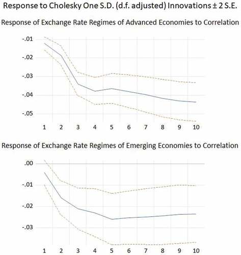
The impulse response functions in Figure 1 show that the comovement of business cycles between advanced countries and emerging countries responds positively and significantly to the exchange rate regimes of these two groups of countries in the short term. However, the positive effect begins to wane before being negative from the third quarter and the fifth quarter for emerging economies and developed economies, respectively. This means that a more flexible exchange rate regime may increase the degree of output correlation in the short run (in the first year), but it decreases in the medium term (in the second year). On the other hand, the exchange rate regimes of both emerging and developed economies respond negatively and significantly to the output correlation. This could be explained by the fact that the monetary policy actors intervene during the high level of output correlation (especially in financial/economic crisis periods) by reducing the degree of flexibility of the exchange rate regime to protect their economy from external shocks. These findings confirm the results obtained by the Granger causality test. Moreover, these results seem valuable since other studies do not directly find these observations, in particular on impulse responses.

Figure 1. Impulse response

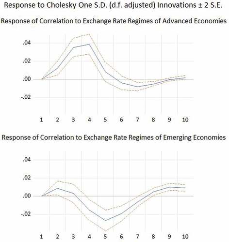
Figure 1. (continued).

5. Conclusion and policy implications

As demonstrated above, this article aims to test the effects of the different exchange rate regimes on business cycles comovement between advanced and emerging countries. It particularly seeks to answer the following question: Does the nature of the exchange rate system affect the degree of output correlation between these economies? To address this question, the present study relied on empirical, discussed the literature related to the different exchange rate systems and output comovement and finally reviewed the methodology and the framework of the empirical analysis.

The starting point to develop the empirical model was to test the stationarity properties of variables via unit root tests on panel data. Then, panel cointegration tests were performed since the variables were not stationary in levels (I 0), but stationary in first differences (I 1). The tests applied were the cointegration tests on panel data of Pedroni (1999, 2004). The results show that the null hypothesis of absence of cointegration cannot be rejected by five tests on the variable $\mathrm{Q}\mathrm{C}\mathrm{O}\mathrm{R}{\mathrm{R}}_{\mathrm{i}\mathrm{j}\mathrm{t}}$ and by the seven tests on the variables $ER{R}_{i,t}$, and $ER{R}_{j,t}$. Therefore, in so far as there is no cointegration relationship between the (non-stationary) variables at level, the empirical properties of the examined variables require the estimation of a Panel VAR model.

We went on to examine the causal relationship by Granger Causality test (VAR modeling) on panel data. This test illustrated the existence of a bidirectional causal relationship between the quasi-correlation of the real GDP growth rates (between emerging and advanced economies) and the exchange rate regimes of these two groups of countries $(ER{R}_{i,t};ER{R}_{j,t}\leftrightarrow QCOR{R}_{ijt})$. Furthermore, Dumitrescu-Hurlin (2012) panel causality test confirms our results.

Finally, the impulse response functions show that the business cycles comovement between advanced countries and emerging countries responds positively and significantly to the exchange rate regimes of these two groups of countries in the short term. However, the positive effect begins to wane before being negative from the third quarter and the fifth quarter for emerging economies and developed economies, respectively. On the other hand, the exchange rate regimes of both emerging and developed economies respond negatively and significantly to the output correlation.

To conclude, the present study is important for several reasons. First, a limited number of previous studies have linked the output comovement to the different exchange rate regimes, especially between advanced and emerging economies. Second, our results seem valuable since other studies do not directly find these observations. Third, the paper produces several policy-related and policy-oriented implications. For example, our main finding shows the existence of a bidirectional causal relationship between output comovement and the exchange rate regimes. For policy implications, this means that exchange rate regime decisions have a significant impact on business cycle co-movement. Also, the output correlation could motivate policymakers to adjust the exchange rate system as an economic policy response. Examples include Indonesia and Hungary in 2008, as well as Poland and Romania during the sovereign debt crisis in 2011. In this context, the transmission channels of monetary policy to the real sphere are numerous. They mainly pass through the interest rate, the credit, and the exchange rate. The effectiveness of monetary policy is conditional on the relative importance of these different channels. Moreover, the transmission channels of monetary policy may be different from one country to another due to the diversity of financial structures. In particular, the same monetary policy measure can lead to different macroeconomic effects depending on the country: a similar decrease in the interest rate from one country to another can lead to a slight increase or a significant growth in demand depending on each country. For example, the implementation of a common monetary policy in Europe could lead to unnecessary biases if the transmission channels differ between the European member countries of the monetary union. Furthermore, if the shocks are idiosyncratic, then the establishment of a monetary union implies a non-negligible cost for its members.

Moreover, monetary policy is linked to exchange rate regimes. Many emerging economies have moved toward more flexible exchange rate regimes. Most monetary policies in this group of countries have changed to allow more monetary autonomy, with inflation-targeting policies. This change has contributed to the stability of prices and the transition of emerging markets’ exchange rate regimes from fixed rate to intermediate and floating rate.

On the other hand, the impulse response illustrates that a flexible exchange rate regime may increase the degree of output correlation in the short run, but it decreases in the medium term. This result could have important implications for policymakers. Hence, flexible exchange rate regime could be adopted to weaken business cycles transmission, especially in recession periods.

Disclosure statement

No potential conflict of interest was reported by the author(s).

Additional information

Funding

The author received no direct funding for this research.

Notes

1. Data refer to Gross Domestic Product (GDP) based on share in world total Purchasing Power Parities (PPP). The source is the International Monetary Fund (IMF), “World Economic Outlook” database, April 2018.

2. The source is the International Monetary Fund (IMF), “World Economic Outlook” report, April 2009.

3. This method is used several times in IMF reports, we can cite as an example “World Economic Outlook”, April 2009, chapter 3.

4. We use the IMF classification. These countries are Austria, Belgium, Cyprus, Estonia, Finland, France, Germany, Greece, Ireland, Italy, Latvia, Lithuania, Luxembourg, Malta, Netherlands, Portugal, Slovakia, Slovenia, Spain, Australia, Canada, Hong Kong, Czech Republic, Denmark, Iceland, Israel, Japan, Korea, New Zealand, Norway, Singapore, Sweden, Switzerland, United Kingdom and United States.

5. We use the IMF, S&P and Dow Jones classifications. These countries are Bangladesh, China, India, Indonesia, Malaysia, Philippines, Thailand, Bulgaria, Hungary, Poland, Romania, Turkey, Russia, Ukraine, Egypt, Pakistan, Qatar, Emirates, South Africa, Argentina, Brazil, Chile, Colombia, Mexico, Peru, and Venezuela.

Appendices

Appendix 1. Reinhart and Rogoff “FINE” classification

Grid	Exchange rate regime
1	No separate legal tender
2	Pre announced peg or currency board arrangement
3	Pre announced horizontal band that is narrower than or equal to ±2%
4	De facto peg
5	Pre announced crawling peg
6	Pre announced crawling band that is narrower than or equal to ±2%
7	De factor crawling peg
8	De facto crawling band that is narrower than or equal to ±2%
9	Pre announced crawling band that is wider than or equal to ±2%
10	De facto crawling band that is narrower than or equal to ±5%
11	Moving band that is narrower than or equal to ±2% (i.e., allows for both appreciation and depreciation over time)
12	Managed floating
13	Freely floating
14	Freely falling
15	Dual market in which parallel market data is missing.

Source: Reinhart and Rogoff (Reinhart et al., 2003)

Appendix 2.

Reinhart and Rogoff “COARSE” classification

Grid	Régimes de change
1	Fixed regime	No separate legal tender
1		Pre announced peg or currency board arrangement
1		Pre announced horizontal band that is narrower than or equal to ±2%
1		De facto peg
2	Limited flexibility	Pre announced crawling peg
2		Pre announced crawling band that is narrower than or equal to ±2%
2		De factor crawling peg
2		De facto crawling band that is narrower than or equal to ±2%
3	Manage floating	Pre announced crawling band that is wider than or equal to ±2%
3		De facto crawling band that is narrower than or equal to ±5%
3		Moving band that is narrower than or equal to ±2% (i.e., allows for both appreciation and depreciation over time)
3		Managed floating
4	Freely floating	Freely floating
5	Freely falling	Freely falling
6	Dual market in which parallel market data is missing	Dual market in which parallel market data is missing.

Source: Reinhart & Rogoff, 2004)

References

- Abiad, A., Furceri, D., Kalemli-Ozcan, S., & Pescatori, A. (2013). Dancing together? Spillovers, common shocks, and the role of financial and trade linkages. In The International Monetry Fund (IMF) World economic outlook (pp. 81–18).
- Artis, Zhang, W., Michael, J., & Zhang. International business cycles and the ERM: Is there a European business cycle? (1997). International Journal of Finance & Economics, 2(1), 1–16. John Wiley & Sons, Ltd. https://doi.org/10.1002/(SICI)1099-1158(199701)2:1<1::AID-IJFE31>3.0.CO;2-7
- Avdjiev, S., McGuire, P., & Wooldridge, P., 2015. Enhancements to the BIS international banking statistics. IFC Bulletin no 39. Bank of International Settlements.
- Baltagi, B., & Kao, C. (2000). Nonstationary Panels, Cointegration in Panels and Dynamic Panels: A Survey. Advances in Econometrics, 15. https://doi.org/10.1016/S0731-9053(00)15002-9
- Baxter, M., & Stockman, A. (1989). Business cycles and the exchange-rate regime: Some international evidence. Journal of Monetary Economics, 23(3), 377–400. https://doi.org/10.1016/0304-3932(89)90039-1
- Bayoumi, T., & Eichengreen, B. (1997, April). Ever closer to heaven? An optimum-currency-area index for European countries. European Economic Review, 41(3–5), 761–770. 1997. https://doi.org/10.1016/S0014-2921(97)00035-4
- Ben David, D., & Papell, D. (1998). Slowdowns and Meltdowns: Postwar Growth Evidence from 74 Countries. The Review of Economics and Statistics, 80(4), 561–571. https://doi.org/10.1162/003465398557834
- Campos, N. F., Coricelli, F., & Luigi, M. (2019). Institutional integration and economic growth in Europe. Journal of Monetary Economics, 103, 88–104. https://doi.org/10.1016/j.jmoneco.2018.08.001
- Céspedes, L. F., Chang, R., & Velasco, A. (2004). Balance sheets and exchange rate policy. American Economic Review, 94(4), 1183–1193. https://doi.org/10.1257/0002828042002589
- Corsetti, G., Dedola, L., Jarociński, M., Maćkowiak, B., & Schmidt, S., 2019. Macroeconomic stabilization, monetary-fiscal interactions, and Europe’s monetary union. European journal of political economy, Elsevier, vol. 57(C), pp. 22–33.
- Darvas, Z., Rose, A., & Szapéry, G., 2005. Fiscal divergence and business cycle synchronization: Irresponsibility is idiosyncratic. Magyar Nemzeti Bank (The Central Bank of Hungary), MNB Working Papers. https://doi.org/10.3386/w11580.
- Dn, G., Porter, D., & Gunasekar, S., 2013. Basic Econometrics. Edition: 5th,Tata McGraw Hill Edu Priv. Ltd.
- DUVAL, R., CHENG, K., HWA, O. H. K., Saraf, R., & Seneviratne, D., 2014. Trade integration and business cycle synchronization: A reappraisal with focus on Asia. IMF Working Paper, WP/14/52.
- Elgahry, B.A. 2014. La synchronisation des cycles économiques entre les pays avancés et les pays émergents: Couplage ou découplage? Thesis dissertation published at le Havre university, France. University of Le Havre, France. https://tel.archives-ouvertes.fr/tel-01132560/document
- Elgahry, B. A., 2016. La synchronisation intra- et inter-régionale des cycles économiques en Europe et en Asie. Revue Interventions économiques, 55. Papers in political Economy. http://journals.openedition.org/interventionseconomiques/2805
- Elgahry, B. A. (2020). Regional and interregional business cycle comovement in Europe, Asia, and North America. Economics Bulletin, 40(4), 3088–3103. https://EconPapers.repec.org/RePEc:ebl:ecbull:eb-20-00472
- Erdem, F. P., & Özmen, E. (2015). Exchange rate regimes and business cycles: An empirical investigation. Open Economies Review, 26 (5), 1041–1058. https://doi.org/10.1007/s11079-015-9361-0
- Findlay, R. (1974). International economics: R.A. Mundell, (Macmillan, New York, 1968). Journal of International Economics, 4(3), 318–319. https://EconPapers.repec.org/RePEc:eee:inecon:v:4:y:1974:i:3:p:318-319
- Frankel, J., & Rose, A. K. The endogeneity of the optimum currency area criteria. (2000). Economic Journal, 108(449), 1009–1025. n°. https://doi.org/10.1111/1468-0297.00327
- Friedman, M. (1953). Essays in positive economics. In Essays in positive economics (pp. 3–43). University of Chicago press.
- Georgiadis, G., & Mehl, A., 2015. Trilemma, not dilemma: Financial globalization and monetary policy effectiveness. Globalization Institute Working Papers 222, Federal Reserve Bank of Dallas.
- Gerlach, Gerlach, H. M. S., & Stefan, H. M. (1988). World Business Cycles under Fixed and Flexible Exchange Rates. Journal of Money, Credit and Banking, Blackwell Publishing, 20(4), 621–632. https://doi.org/10.2307/1992288
- Granger, C. (1969). Investigating causal relations by econometric models and cross-spectral methods. Econometrica, 37(3), 424–438. https://doi.org/10.2307/1912791
- Harding, D., & Pagan, A., 2006. Measurement of business cycles. Department of Economics - Working Papers Series, the University of Melbourne 966.
- Holtz-Eakin, D., Newey, W., & Rosen, H. S. (1988). Estimating Vector Autoregressions with Panel Data. Econometrica, 56(6), 1371–1395. https://doi.org/10.2307/1913103
- Hou, J., & Knaze, J. 2019. The effect of exchange rate regimes on business cycle synchronization: A robust analysis. MPRA paper: Munich Personal RePEc Archive. https://mpra.ub.uni-muenchen.de/95182/1/MPRA_paper_95182.pdf
- Hurlin, C., & Mignon, V. (2005). Une synthèse des tests de racine unitaire sur données de panel. Économie & Prévision 2005/3-4-5, 253–294.
- Ilzetzki, E., Reinhart, C., Rogoff, K., & National bureau of economic research, inc. 2017. Exchange arrangements entering the 21st century: which anchor will hold?NBER Working Papers No 23134.
- Im, K. S., Pesaran, M. H., & Shin, Y. (1997). Testing for Unit Roots in Heterogeneous Panels. Cambridge: Department of Applied Economics, University of Cambridge.
- Jiang, W., Yunong, L., & Zhang, S. (2019). Business cycle synchronization in East Asia: The role of value‐added trade. The World Economy, 42(1), 226–241. https://doi.org/10.1111/twec.12668
- Kalemli-Ozcan, S., Papaioannou, E., & Peydro, J. L. (2013). Financial regulation, financial globalization and the synchronization of economic activity. Journal of Finance, 68 (3), 1179–1228. https://doi.org/10.1111/jofi.12025
- Klein, M., & Shambaugh, J., 2010. Exchange rate regimes in the modern era: https://mitpress.universitypressscholarship.com/view/10.7551/mitpress/9780262013659.001.0001/upso-9780262013659-chapter-1
- Kwack, S. Y. (2004). An optimum currency area in East Asia: Feasibility, coordination, and leadership role. Journal of Asian Economics, 15(1), 153–169. https://doi.org/10.1016/j.asieco.2003.12.006
- Levin, A., Lin, C.-F., Chu, J., & C.-S. (2002). Unit root tests in panel data: Asymptotic and finite-sample properties. Journal of Econometrics, 108(1), 1–24. https://doi.org/10.1016/S0304-4076(01)00098-7
- Levy-Yeyati, E., & Sturzenegger, F. (2005). Classifying exchange rate regimes: Deeds vs. Words. European Economic Review, 49(6), 1603–1635. https://doi.org/10.1016/j.euroecorev.2004.01.001
- Li, H., Xu, L. C., & Zou, H.-F. (2000). Corruption, Income Distribution, and Growth. Economics & Politics, 12, 155–182. https://doi.org/10.1111/1468-0343.00073
- Mahembe, E., & Odhiambo, N. M. (2019). Foreign aid, poverty, and economic growth in developing countries: A dynamic panel data causality analysis. Cogent Economics & Finance, 7:1(1), 1626321. https://doi.org/10.1080/23322039.2019.1626321
- Mitchell, W. C., 1927. Business cycles: The problem and its setting. National Bureau of Economic Research : https://www.nber.org/books-and-chapters/business-cycles-problem-and-its-setting
- Narayan, P., & Narayan, S. (2010). Carbon dioxide emissions and economic growth: Panel data evidence from developing countries. Energy Policy, 38(1), 661–666. https://EconPapers.repec.org/RePEc:eee:enepol:v:38:y:2010:i:1:p:661-666
- Passari, E., & Rey, H., 2015. Financial flows and the international monetary system. CEPR Discussion Paper No. DP10592: https://ssrn.com/abstract=2608050
- Pesce, A., 2015. Economic Cycles in Emerging and Advanced Countries Synchronization, International Spillovers and the Decoupling Hypothesis. Springer. https://link.springer.com/book/10.1007/978-3-319-17085-5
- REINHART, C., & REINHART, V., 2008. Capital flow bonanzas: An encompassing view of the past and present. Paper prepared for the NBER International Seminar in Macroeconomics, June 20–21: www.cepr.org/pubs/new-dps/dplist.asp?dpno=6996.asp
- Reinhart, C., & Rogoff, K. (2004). The modern history of exchange rate arrangements: A reinterpretation. The Quarterly Journal of Economics, 119(1), 1–48. https://doi.org/10.1162/003355304772839515
- Reinhart, C. M., Rogoff, K. S., & Savastano, M. A., 2003. Debt intolerance. Brookings Papers on Economic Activity, 341, 1–74. https://EconPapers.repec.org/RePEc:bin:bpeajo:v:34:y:2003:i:2003-1:p:1-74
- Rey, H., 2013. Dilemma not trilemma: The global cycle and monetary policy Independence. Proceedings - Economic Policy Symposium - Jackson Hole, Federal Reserve Bank of Kansas City, pp. 1–2.
- Rey, H. (2016). International channels of transmission of monetary policy and the mundellian trilemma. IMF Economic Review, 64 (1), 6. https://doi.org/10.1057/imfer.2016.4
- Rose, A., & Spiegel, M. (2009). International financial remoteness and macroeconomic volatility. Journal of Development Economics, 89(2), 250–257. https://doi.org/10.1016/j.jdeveco.2008.04.005
- Sato, K., & Zhang, Z. (2006). Real output co‐movements in East Asia: Any evidence for a monetary union? The World Economy, 29(12), 1671–1689. https://doi.org/10.1111/j.1467-9701.2006.00863.x
- Shin, K., & Wang, Y., 2003. Monetary integration ahead of trade integration in East Asia? ISER discussion paper 0572, Institute of Social and Economic Research, Osaka University.
- Smith, I. (2003). The Law and Economics of Marriage Contracts. Journal of Economic Surveys, 17, 201–226. https://doi.org/10.1111/1467-6419.00193
- Turnovsky, Turnovsky, S. J., & Stephen, J. (1976). The relative stability of alternative exchange rate systems in the presence of random disturbances. Journal of Money, Credit and Banking, Blackwell Publishing, 8(1), 29–50. https://doi.org/10.2307/1991918
- Wald, A. (1943). Tests of Statistical Hypotheses Concerning Several Parameters When the Number of Observations is Large. Transactions of the American Mathematical Society, 54(3), 426–482. https://doi.org/10.2307/1990256
- Wooldridge, 2013. Introductory econometrics: A modern approach: https://economics.ut.ac.ir/documents/3030266/14100645/Jeffrey_M._Wooldridge_Introductory_Econometrics_A_Modern_Approach__2012.pdf
- Wyplosz, C., 2001. How risky is financial liberalization in the developing countries? CEPR Discussion Papers, No 2724.
- Yougbaré, L., 2009. Effets macroéconomiques des régimes de change: Essais sur la volatilité, la croissance économique et les déséquilibres du taux de change réel. Thesis dissertation published in: Université Clermont-Ferrand 1.