Impact of economic sectors on inflation rate: Evidence from Ethiopia

Abstract

It is unclear how sectoral growth in the agriculture, industrial, and service sectors affects inflation, and the topic is also quite rare. Accordingly, the researchers in this paper examine the long- and short-term effects of agriculture, service, and industry sectors on inflation rates. In order to achieve this, the researchers applied an autoregressive distributed lag model from 1975 to 2019. In order to determine the direction of causation, the Granger causality test was conducted. The results clearly demonstrate the negative relationship between agriculture, services, population, and inflation over the long term. In the short run, previous inflation, the service sector, the second lag in population, and the agricultural sector do not reduce inflation. The industrial sector and the first lag of the population can lower inflation rates. Thus, the industry sector in the long run and the service and agricultural sectors in the short run are inefficient at reducing inflation. Inflation and the agricultural sector are causally linked in both directions. Additionally, unidirectional causality runs from industry and the service sector to inflation. Early researchers have not examined the impact of the service, industry, and agriculture sectors on inflation rate, thus offering a unique contribution to policy makers. Panel data are not used to compare the sectoral responsibility for reducing inflation in other African countries with researchers. Practically, the agriculture and service sectors on the short run, along with the industry sector on the long run, both need attention.

Keywords:

• agriculture sector
• Ethiopia
• inflation rate
• industry sector
• service sector

JEL Classifications:

• E23
• E31
• L8
• Q1

PUBLIC INTEREST STATEMENT

The inflation rate can be used as a gauge of an economy’s health. The impact of economic sectors on inflation rate is rarely examined empirically. This paper fills the gap by looking into the long- and short-term effects of economic sectors on inflation rates. Agriculture, service, and population have a negative relationship with inflation over the long run. On the short run, industrial growth can lower inflation rates. Agriculture and inflation are causally linked in both directions. Furthermore, unidirectional causality runs from industry and the service sector to inflation. In three ways, our paper differs from past research. The study uses long-term data to focus on economic sectors for the first time. Our study also uses advanced econometrics for the long run and short run. Thirdly, this study uses economic sectors as independent variables, offering a unique contribution to policy makers and raising the question of which sector needs more focus in order to control Ethiopia’s alarming rates of inflation. On the short term, agriculture and services need attention, as do industries on the long-term.

1. Introduction

Macroeconomic policymakers and academics consider controlling inflation to be an imperative objective. Researchers have focused on inflation as one of their most relevant topics; however, the challenge of inflation has been a perpetual headache for policy makers. It is commonly believed that inflation occurs when too much money pursues too few goods (Lim & Sek Siok, 2015). Due to changes in the structure of the economy, strategic deficiencies and so-called bottlenecks in supply channels emerge. A bottleneck can occur if supply for a given good suddenly increases (Argy, 1970; Olivera, 1964).

Stability in key macroeconomic variables is essential for economic growth. Stabilized macroeconomic variables play a significant role in determining the overall economic environment. According to monetary theory and modern economic literatures, the price level is one of the most important macroeconomic variables. Beyond the optimum level, inflation is ruthless. Moreover, it adversely affects the welfare of the public; especially the poor (Yamaguchi, 2013). In order to deal with the impact of inflation on economic growth, policy makers need to control its level. A sharp increase in inflation could reduce economic growth and exacerbate poverty (Melaku, 2020).

It remains the primary goal of macroeconomic policies to achieve sustainable growth while maintaining price stability. A high inflation level is detrimental to economic growth (Seleteng, 2013). Since 2008, the high inflation rate has also been a headache for the Ethiopian government due to its repercussions on people’s living standards. In 2019/20, headline inflation increased to 19.9 percent from 12.6 percent a year earlier (NBE, 2019). According to Mekonen (2020), the relationship between inflation and sectoral growth is useful, because it benefit of obtaining evidence from a variety of sectors is identifying growth patterns and economic policy transmission channels. This suggests that investigating the impact of sectoral growth on inflation has theoretical as well as practical relevance. Sectoral growth is seen as vital in Ethiopia due to the majority of Ethiopians’ reliance on it to support themselves.

During the 2017/18 Ethiopian fiscal year, agriculture, industry, and services contributed 35%, 27%, and 39% of GDP, respectively, compared to 36.3%, 26%, and 38.8% during the previous fiscal year (NBE, 2018). The sector contributed 42.6% to the overall economic growth during the fiscal year. The service sector remained dominant in the economy with a share of GDP of about 39.5 percent (NBE, 2019). Having this contribution to economic growth, but empirically there is no efficient study about the contribution of sectoral growth to the reduction of inflation.

In addition, previous studies have been conducted, but typically they provide a narrow view, for example, (Alemu et al., 2003; Block, 1999; Faridi, 2012; Hussin & Yik, 2012; Kaur, 2019; Kaur & Aggarwal, 2013; Mekonen, 2020; Mkhatshwa et al., 2015; Ndour, 2017; Olaniyi et al., 2015; Oyakhilomen & Rekwot, 2014; Xinshen & Steven, 2007; Zulfiqar, 2015), we found them to be less explored in the literature, at least in terms of how economic sectors affect inflation. Literature reviews have also been conducted on inflation in several countries, but most of these studies focused on macroeconomic determinants rather than the impact of sectoral growth, for example, (Bane, 2018; Kahssay, 2017; Melaku, 2020).

According to research conducted by Mekonen (2020), inflation in Ethiopia is detrimental to agriculture sector growth rather than stimulating it. Chaudhry et al. (2013) found that inflation hinders the growth of the manufacturing sector, while it’s statistically significant positive impact encourages the growth of the services sector. It has been observed that inflation and agriculture sector growth are positively and significantly related. The study by Ayyoub (2015) showed that inflation has a positive effect on agriculture sector growth. Kaur (2019), however, found the negative impact of inflation on India’s agriculture sector. According to Mkhatshwa et al. (2015), inflation was negatively related to agricultural sector growth in Swaziland. In a study by Oyakhilomen and Rekwot (2014), the trend of inflation has had a significant impact on agricultural productivity.

In contrast, it is unclear how sectoral growth in the agricultural, industrial, and service sectors affects inflation, and the topic is also quite rare. Hence, examining sectoral growth and inflation could provide new insights for policy makers to design effective economic policy. As far as the researcher knows, in Ethiopia the impact of sectoral growth on inflation rate has been neglected, and studies have not been conducted.

This study provides a useful contribution to the empirical basis necessary for understanding the previous routes and focusing future efforts on inflation rates. Furthermore, the study contributes to the stock of knowledge by showing the relationship between inflation and sectoral growth in the Ethiopian economy. Few researchers have conducted specific research on it, yet it is considered as an introduction to the topic. There has been a lot of research on macroeconomic determinants of inflation around the world. However, Ethiopia is not well represented in the literature and specifically the impact of sectoral growth on inflation has not been fully examined. Studying the causal relationships between variables is extremely useful since it provides useful information on what economic variables the government and relevant authorities need to control. As a result, they aim to achieve the desired level of the targeted variables. Inflation and sectoral growth have significant implications for the state of the economy. For example, if the results of the causality test indicate that sectoral growth causes inflation, then governments and policy makers can design policies to manage the growth of sectors in order to achieve a lower inflation rate. Likewise, if econometric investigation reveals the opposite, then efforts would be made to remove obstacles so that high inflation can be curtailed. The study provides detailed ideas and helpful directions for policymakers, economists, and researchers who are keenly interested in inflation. In addition, Ethiopia’s government has set a goal to achieve middle-income status by 2025. To continue Ethiopia’s successful journey towards becoming a middle income country, the results from the research will be used as input. Likewise, taking into account the findings of this research also plays an imperative role in evaluating the second Growth and Transformation Plan (GTP II).

1.1. Research questions

In this study, we critically explored the following research questions regarding the relationship between inflation rate and sectoral growth in Ethiopia during the period of study.

1. Is there any long run relationship between inflation rate and sectoral growth in Ethiopia from 1975 to 2019?

2. Is there any short run relationship between inflation rate and sectoral growth in Ethiopia from 1975 to 2019?

3. Is there a causal relationship between inflation rate and sectoral growth in Ethiopia from 1975 to 2019?

1.2. Objective of the study

Thus, the objective of this study is to investigate the impact of economic sectors on inflation rate at a national level using annual data (1975–2019). And it has the following specific objectives.

1. To investigate the long run relationship between inflation rate and sectoral growth in Ethiopia from 1975 to 2019.

2. To examine short run relationship between inflation rate and sectoral growth in Ethiopia from 1975 to 2019.

3. To show a causal relationship between inflation rate and sectoral growth in Ethiopia from 1975 to 2019.

1.3. Research hypotheses

According to the researchers, the research hypotheses have been developed to achieve the objectives of this study.

1. There is a negative relationship between the inflation rate and sectoral growth in Ethiopia over the long- and short-run.

2. There is a causal link between the macroeconomic variables mentioned in the study.

1.4. Scope of the study

In terms of coverage, it was limited to Ethiopian economy. There is a lack of well documented time series data for long time periods in developing countries, so the secondary data understudy is limited to last 1975–2019 years. Sectoral growth should be considered in this analysis as a macroeconomic variable impacting inflation in Ethiopia. As a result of a small sample size, and to avoid losing degree of freedom, this study is limited to a few determinants, while other macroeconomic variables may be included, but except for a few studies on the impact of sectoral growth, most of the other macroeconomic variables, i.e. money supply, exchange rate, government expenditure, tax revenue, budget deficit, external debt, interest rate, trade openness, unemployment, investment and economic growth are covered very well by previous studies, for instance, Alemu et al. (2016), Kahssay (2017), Yismaw (2019), Emeru (2020), Sirah (2020), Melaku (2020), and Denbel et al. (2016).

1.5. Organization of the study

Following is the organization of the paper. In section two, the literature reviews are summarized, in section three, the methodologies are presented, in section four there are results and discussion, and in section five, the conclusions, policy recommendations, and future directions are discussed.

2. Review of literature

According to orthodox policy prescription, the quantity theory of money provides the dominant conceptual framework to interpret contemporary financial events and provides the intellectual foundation of the 19th century classical monetary analysis (I. Fisher, 1911). Hume (1752) was the first to analyze how monetary factors spread from one sector of the economy to another, changing relative price and quantity. The quantity theory of money was refined, elaborated and extended by him.

The money supply is considered to be the main determinant of both the level of output and prices in the short run, as well as the level of prices in the long run, by monetarists. In the long run, the money supply has no effect on output (Friedman & Schwartz, 1963). Money played an imperative role for monetarists. During the post-war period, Milton Friedman developed the quantity theory of inflation which held that “inflation is always and everywhere a monetary phenomenon, and arises when more money is made than is produced by a nation’s total output”. Monetarists used Fisher’s identification of the exchange equation to come up with the earliest explanation of money.

At full employment, there will be an inflationary gap when aggregate demand exceeds aggregate supply. Inflation is more rapid when there is a significant gap between aggregate supply and demand. The Keynesian demand-pull inflationary theory proposes that a policy that causes a decline in each component of total demand is effective in reducing inflationary pressures. In terms of reducing government expenditure, a tax increase and the control of the volume of money individually or in tandem can be effective in taming inflation and reducing demand. Hyperinflation during a war, for example, when the control of money volume or the reduction in general spending may not be possible, an increase in tax can provide direct control of demand (Keynes, 1936).

Generally, cost-push inflation occurs when unions enforce wage increases and employers increase profit margins. Inflation of this type has been a phenomenon for centuries, dating back to the middle Ages. However, it was reevaluated in the 1950s and again in the 1970s as a cause of inflation. Money wages rise faster than labor productivity, resulting in cost-push inflation (Humphrey, 1998).

A structural factor affects inflation. An economy structure analysis aims to understand how macroeconomic phenomena develop, and to identify the cause of an enduring disease, such as inflation. It also aims to determine the appropriate relationship between them. When unemployment is high and production factors are slow, these structural factors cause a rise in supply related to demand-push. In light of this, the thinking of less developed countries has not been able to change in a way in which they have lagged behind on structure, neglected to engage in immediate self-economic growth, or compromised with sometimes very severe inflation. Inflation is considered as a cost of immediate economic growth due to structural improvements. Another inflationary factor is the rapid and faster growth of the service sector as a result of population growth and immigration (Canavese, 1982).

In the 1970s, rational expectations theory dominated macroeconomics (Humphrey, 1998; Lucas, 1972; McCallum, 1980; Sargent & Hansen, 1980). As the rational expectation school argued, people don’t make the same forecasting errors as implied in the adaptive expectation idea. Based on the monetarist assumption of continuous market clearing and imperfect information, this is true. The macroeconomic expectations of economic agents can be called logical if they are based on current and past relevant information, rather than only on past information as in case of backward-looking or adaptive price expectations.

Because of the new Keynesian assumption of price stickiness in the short run, monetary or demand factors play a key role in determining business cycles in the new neoclassical synthesis. In parallel, the new neoclassical synthesis suggests that supply shocks may play a significant role in explaining real economic activity, as suggested in the new classical real business cycle theory .

A. H. Khan and Qasim (1996) food inflation is determined by three factors: money supply, manufacturing value-added, and wheat support price. Prices of imports, electricity, and the money supply are factors that influence non-food inflation. Chaudhry et al. (2013) found that inflation is negatively related to the manufacturing sector, but positively related to the service and agricultural sectors. Loto (2012) argues that inflation and lending rates are not significantly related to manufacturing performance. Based on Lindh and Malmberg (2000)’s research, an aging population leads to net savings and low inflation, while a young population leads to high consumption and high inflation.

In contrast, Kaur (2019) argued that inflation has a negative impact on agriculture sector growth in India, a finding contested by Ayyoub (2015). Mkhatshwa et al. (2015) demonstrated that inflation negatively influenced agriculture sector growth in Swaziland. Oyakhilomen and Rekwot (2014) showed that inflation affected agricultural productivity to a significant degree. Thus, the findings from various literatures indicate that there is a plethora of mixed evidence regarding inflation’s effect on agriculture growth. In this regard, a large part of the variance may be related to the different approaches taken by researchers. Nawaz et al. (2017) determined that it is the money supply, government expenditure, government revenues, and foreign direct investment that have positive impacts on inflation within Pakistan. Jaffri et al. (2016) concluded that population growth is significantly responsible for rising inflation. The empirical evidence discussed above indicates that other macroeconomic factors are given a lot of attention, rather than sectoral growth. However, the effects of sectoral growth on inflation in both developed and developing countries are not well documented. So, there is a gap in the literature, and this study aims to fill that gap.

Durguti et al. (2021) investigated the effects of macroeconomic determinants on inflation in the Western Balkans. In the short run, all variables influence inflation rate, except foreign direct investment, which has a negligible effect. Furthermore, Arellano-Bover/Blundell-Bond estimations indicate that GDP growth, imports, and foreign direct investments affect inflation positively, and that exports and working remittances negatively affect inflation. Using a time series of data spanning from 1975 to 2017, Degu (2019) examined the inter-sectoral links in Ethiopia’s economy. In the long run, the agricultural, industrial, and service sectors of the economy have a stable relationship. It has been found that only the industrial sector is endogenous to the system, implying a long-run causality from agriculture and service sectors to industrial sectors. Short run Granger causality results show that the industrial and agricultural sectors are bidirectional.

2.1. Overview of inflation in Ethiopia

In 1974, a popular revolution toppled the imperial regime and brought the Derg to power. Derg economics was characterized by a socialist ideology that subjugated market forces and systematically socialized production and distribution. Moreover, a strong dependence on agriculture, which is subject to the vagaries of nature, led to an irregular growth rate (Alemayehu, 2003a). Furthermore, it was also marked by intense conflict, which aggravated the dismal economic performance of the Derg regime. The monetary variables in Ethiopia during the command era were directly regulated by the monetary authorities. Since the Derg regime, Ethiopia’s inflation rate has been low due to the government’s control over prices and the government’s provision of goods at fixed prices. Another factor that has helped lower inflation rates is the lower and fixed exchange rate. From 2006 to 2015, Ethiopia had an average inflation rate of 18.69 percent.

Following the downfall of the Derg regime and the rise of the Ethiopian People’s Revolutionary Democratic Front to power in Ethiopia, the focus shifted from direct command over monetary variables to market-based policy instruments, as the government left economic policy to the private sector (Chewaka, 2014). This in turn gave rise to price fluctuations in the economy. During war and drought, general prices rose dramatically. In the Imperial era, the military regime, and the first decade following Derg’s death, the consumer price index increased by an average of 3.5, 8.8, and 5.3 per cent per year, respectively.

Following the change in the government’s monetary and fiscal policy and the government’s activism in the economy, inflation began to threaten the economy in the post-2002/03 period (Tafere, 2008). Until 2003, Ethiopia had an inflation rate in the single digits, except in years of supply shocks and war. As an example, between 1971 and 2003, inflation averaged 7.5%. During this time, the highest inflation rate of 45% occurred in 1991, the first year the Ethiopian People’s Revolutionary Democratic Front came to power after the end of the civil war. Nonetheless, between 2004 and 2014, inflation rates increased rapidly and the average inflation rate in this period reached 17.7% with the highest rate of 39.5% registered in 2008. Accordingly, the highest inflation episodes occurred in 1984/85 and 2003 as a result of drought, and in 1991/92 as a result of war (Loening et al., 2009).

Compared to a year earlier, headline inflation increased to 19.9 percent in 2019/20 (NBE, 2019). As a result of their study, Getachew and Meaza (2018) have determined the optimal level of inflation in Ethiopia that affects economic growth most positively. In this study, thresholds were applied. For Ethiopia, a rate of inflation of about 9%-10% is optimal. Economic growth may not be possible if inflation is higher or lower than the threshold level. Recently, double-digit inflation has become worrisome for policy makers and society alike, even though Ethiopia has experienced a low inflation rate and good economic performance. In March 2022, Ethiopia’s annual inflation rate increased to 34.7%, up from 33.6% the previous month. A temporary price cap for food items and a three-month ban on rent increases by landlords were recently implemented to control inflationary pressures, but the reading was the highest since December last year. Both food prices (43.4% vs 41.8% in February) and non-food items (23.5% vs 22.9%) were up. Consumer prices inched up 4% on a monthly basis, the most significant jump in six months (CSA, 2022).

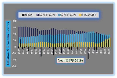
The proportion of agricultural output in GDP declined steadily from nearly 70 percent in 1960/61 to nearly 50 percent in 1973/74 during the imperial period—this was a positive trend. Within the second (Derg) administration, the decline halted at roughly 50 percent of GDP. Despite this upward trend in services, the value of industrial value-added did not change significantly during the Derg period. There have been no noticeable changes in the economy during the Derg era, with the exception of the service sector. Accordingly, agriculture contributed 52.5 percent of the country’s GDP in 1973/74 and remained at 50.9% at the end of the Derg era (1989/90). As of the end of the third period (1999/2000), this figure has declined to 43.2%, primarily due to an increasing share of services. Based on Figure 1, over the entire period, the share of industry appears to have stagnated at around 13 %. Thus, although the share of each sector fluctuates in a very narrow band, it has remained constant in the last four decades. Agriculture (34.9%), industry (27%), and services (39%) all contributed to economic growth in 2017/18 (NBE, 2017).

Figure 1. Graphical view of economic variables.

3. Methodology

3.1. Data source and type

Time series annual data were used for this study. The variables included were services (% GDP), industry (% GDP), agriculture (% GDP), and population growth (%) for Ethiopia over the period 1975–2019. Inflation rate of Ethiopia as measured by consumer price index (CPI). Policy makers’ ultimate objective is to attain rapid economic growth and stabilize the price level (Mekonen, 2020). Three main sources of data were used: the World Bank (WB), the Ministry of Finance and Economic Development (MoFED), and the National Bank of Ethiopia (NBE). It is well known that these databases contain up-to-date, robust, comprehensive and reliable annual data because studies have relied on data published by WDI, MoFED, and NBE (Bane, 2018; Melaku, 2020; Sisay et al., 2020).

Phillips (1958) observed that the rate of inflation and unemployment rate were negatively related. An empirical specification of the Philips curve is presented in equation 1.

(1) $IN{F}_t=f(UN{R}_t$(1)

In which,

INF: inflation rate

UNR: unemployment rate

t: time subscript (year)

Basically Okun (1962) examined the relationship between unemployment rate and economic growth. If GDP grows rapidly, the unemployment rate declines. This is shown in equation 2(2) $UN{R}_t=f(GD{P}_t)$(2) .

(2) $UN{R}_t=f(GD{P}_t)$(2)

In which,

GDP: gross domestic product

Economic sectors are linked to each other and to economic growth. Economic development and structural change are linked hand-in-hand. However, an economy may experience such temporal changes in the composition of different sectors and subsectors in terms of productivity and employment levels if distortionary policies are pursued, which might result in unbalanced growth, each within its own sector (Xinshen & Steven, 2007). The primary, secondary, and tertiary sectors of the economy were classified by G.B.A. Fisher (1935) and Clark (1940). The distribution gives an overview of agriculture, industry, and services, which each contribute a percentage of GDP (NBE, 2019). Its functional expression as seen in the equation 3(3) $UN{R}_t=f(GD{P}_t)=f(S{S}_t,I{S}_t,A{S}_t)$(3) .

(3) $UN{R}_t=f(GD{P}_t)=f(S{S}_t,I{S}_t,A{S}_t)$(3)

In which,

SS: service sector (%GDP)

IS: industry sector (%GDP)

AS: agriculture sector (%GDP)

Once appreciation is gained of the important role that other variables play in explaining inflation, it is important to include them in the model to study its impact on inflation, i.e. population growth. Africa’s second-most populous nation after Nigeria is Ethiopia, which also has the fastest-growing economy. There is a lack of consensus regarding whether population growth drives healthy economic growth, even though this issue continues to be of intense importance for policy-making, particularly in developing nations (Ukpolo, 2002). In fact, Malthus (1798) suggested that unrestrained population growth could negatively influence economic growth through its influence on important determinants such as the savings rate, natural resources, capital formation, and the environment.

According to other studies, population growth may actually improve a society’s economic conditions and reduce poverty through the contribution of innovative ideas. With the increase in population, Keynes states, a good market can be established as well as the demand for capital will increase. Optimists such as Lewis (1954) have declared that population growth will increase economic growth. According to Bogue (1982), improved technology can boost production. For this reason, the researchers included population as an independent variable. This is shown in equation 4(4) $INF{R}_t=f(UN{R}_t)=f(GD{P}_t)=f(S{S}_t,I{S}_t,A{S}_s,PO{P}_t)$(4) .

(4) $INF{R}_t=f(UN{R}_t)=f(GD{P}_t)=f(S{S}_t,I{S}_t,A{S}_s,PO{P}_t)$(4)

3.2. Rationality for log transformation of variables

Further, some observations of inflation rate were negative, so to convert them to logarithmic form, this study applied equation 5 (Busse & Hefeker, 2007).

(5) $\mathrm{y}=\mathrm{l}\mathrm{n}(\mathrm{x}+\sqrt{{\mathrm{x}}^2+1}$(5)

In which,

Ln: logarithm expression of variables

y and x: represent a specific economic variable

Although not all of the variables in the model can be controlled, it uses various sources to consider the effects of the other shocks, so we consider the error term.

The equation for the log transformation is as follows. It is presented as the following equation 6(6) $INF{R}_t={\beta }_{0}S{S}_t^{{\beta }_1}I{S}_t^{{\beta }_2}A{S}_t^{{\beta }_3}{\beta }_{4}PO{P}_t{e}^{\mu t}$(6) .

(6) $INF{R}_t={\beta }_{0}S{S}_t^{{\beta }_1}I{S}_t^{{\beta }_2}A{S}_t^{{\beta }_3}{\beta }_{4}PO{P}_t{e}^{\mu t}$(6)

Transforming variables into their natural logarithm form has two major advantages. First, the slope coefficients of non-logarithmic linear equations measure only the rate at which the dependent variables mean changes. The slope coefficient is, however, more useful when variables are transformed to their natural logs so that it can measure both change in the mean as well as elasticity of the dependent variable as a function of the change in the independent variables. Additionally, the log transformation reduces the problem of heteroscedasticity by compressing the scale from which variables are measured (Gujarati, 2004).

The log-log forms of the models can be stated as equation 7(7) $LnINF{R}_t={\beta }_0+{\beta }_{1}LnS{S}_t+{\beta }_{2}LnI{S}_t+{\beta }_{3}LnA{S}_t+{\beta }_{4}LnPO{P}_t+{\mu }_t$(7) .

(7) $LnINF{R}_t={\beta }_0+{\beta }_{1}LnS{S}_t+{\beta }_{2}LnI{S}_t+{\beta }_{3}LnA{S}_t+{\beta }_{4}LnPO{P}_t+{\mu }_t$(7)

LnPOP: Population growth rate (%)

μt: the error term

${\beta }_{1}to{\beta }_4$: are the parameters and the elasticity’s of the independent variables

${\beta }_0$: as a constant term, the dependent variable assumes a value of zero if all the independent variables are zero or near zero.

Data are analyzed based on empirical estimates obtained using econometrics and statistics, i.e., the E-views statistical package.

3.3. Assumption of the study

The dynamics of sectoral shares are interrelated to each other and with economic growth. The economy’s development and structural changes are known to go hand-in-hand. If faced with distortionary policies, an economy might, however, witness such temporal changes in the composition of different sectors and sub-sectors in productivity and employment level which could lead to unbalanced growth within sectors. Firstly, sectoral growth will lead to stable economic growth, and secondly, if economic growth is stable, inflation will decrease. Moreover, structural inflation theory states that inflation is a function of agricultural, financial, industrial and physical infrastructure development. Accordingly, this study was conducted with this mindset.

3.4. Stationary test

Neither forecasting nor hypothesis testing can be done using regression on non-stationary series. The ADF test is used to check the stationary behavior of each variable as well as to check the order of integration. Therefore, the Augmented Dickey-Fuller (ADF) test is applicable (Dickey & Fuller, 1979). A number of important statistical tests are available for large time series, including the Kwiatkowski-Phillips-Schmidt-Shin (KPSS), the Phillips-Perron (PP) test and the Ng-Perron (NP) test (Arltová & Fedorová, 2016; Sisay et al., 2020). For this reason, this study used ADF test statistics. A lag length criterion is selected by a majority vote based on the minimum value of each criterion and by considering the familiar criterion that is used for economics research as well (Ng & Perron, 2001). To eliminate autocorrelation among residuals, ADF contains an extra lagged term of the dependent variable. In the ADF test, three different regression equations (equation 8(8) $\mathrm{\Delta }{X}_t=\gamma X_{t-1}+{\sum }_{i=1}^p{\beta }_i\mathrm{\Delta }X+e_t$(8) , 9(9) $\mathrm{\Delta }{X}_t={\alpha }_0+\gamma X_{t-1}+{\sum }_{i=1}^p{\beta }_i\mathrm{\Delta }X+e_t$(9) and 10(10) $\mathrm{\Delta }{X}_t={\alpha }_0+\gamma X_{t-1}+\theta T+{\sum }_{i=1}^p{\beta }_i\mathrm{\Delta }{X}_{t-i}+e_t$(10) ) are used to test for the existence of a unit root.

• Without drift and trend

(8) $\mathrm{\Delta }{X}_t=\gamma X_{t-1}+{\sum }_{i=1}^p{\beta }_i\mathrm{\Delta }X+e_t$(8)

• With intercept

(9) $\mathrm{\Delta }{X}_t={\alpha }_0+\gamma X_{t-1}+{\sum }_{i=1}^p{\beta }_i\mathrm{\Delta }X+e_t$(9)

• With drift and trend

(10) $\mathrm{\Delta }{X}_t={\alpha }_0+\gamma X_{t-1}+\theta T+{\sum }_{i=1}^p{\beta }_i\mathrm{\Delta }{X}_{t-i}+e_t$(10)

In which,

$\mathrm{\Delta }$: difference operator

${\alpha }_0$: drift term

P: the lag order of the auto-regressive process

T: trend term/trend variable

t: time subscribe

${\beta }_i$: a measure of lag length

$\gamma$: the coefficient of $X_{t-1}$ which measures the unit root

e: the error term

$\theta$: the coefficient on a time trend series

$\mathrm{\Delta }{X}_t:$ first difference of $X_t$

$X_{t-1}$: lagged values of order one of $X_t$

$\mathrm{\Delta }{X}_{t-i}:$ are changes in lagged values

$\mathrm{\Delta }{X}_{t-1}=X_{t-1}-X_{t-2}$

The null and alternative hypotheses can be written as follows:

$H_o$: $H_o$ Non-stationary time series, so it has unit root problem.

$H_a$: $\gamma <0,$ Stationary time series, so it has not unit root problem.

In the event that t-statistics are greater than ADF critical value, the null hypothesis will be rejected. ADF critical value must be less than t-statistics for the null hypothesis to be rejected (Sirah et al., 2021; Sisay et al., 2020).

3.5. An autoregressive distributed lag model

In the ARDL technique, endogeneity is less of an issue because it is free from residual correlation (i.e. all variables are assumed to be endogenous). We can also analyze the reference model using it. In addition, the ARDL method can distinguish between explanatory and dependent variables and eliminate problems caused by autocorrelation or endogeneity (Afzal et al., 2013).

According to Omoniyi and Olawale (2015), another condition for using ARDL is that all variables under study do not have to be integrated in the same order. It can be applied to variables integrated of order one or zero, as in this study. Another advantage is that, for small and finite data samples (30 to 80), the ARDL test is relatively more efficient. As a third benefit, we obtain unbiased estimates of the long-run model by applying ARDL (Harris & Sollis, 2003). In addition, the ARDL procedure allows differentiating between explanatory variables and dependent variables. It means that the ARDL approach assumes a single reduced form equation relationship exists between the dependent variable and the exogenous variables (M. Hashem Pesaran et al., 2001).

In order to determine whether the variables are co-integrated or not, or are inconclusive, the researcher must compare the calculated F-statistics value (Wald test) with the critical values reported in the paper (M.H. Pesaran et al., 1999). M.H. Pesaran et al. (1999) introduced the ARDL model, which was further explained by M. Hashem Pesaran et al. (2001). Equation 11(11) $Y_t^{,}={\gamma }_{0i}+{\sum }_{i=1}^P{\delta }_i{Y}_{t-i}+{\sum }_{j=0}^q{\beta }_i^{,}{X}_{t-i}+{\epsilon }_{ti}$(11) illustrates ARDL (p, q) in a general form.

(11) $Y_t^{,}={\gamma }_{0i}+{\sum }_{i=1}^P{\delta }_i{Y}_{t-i}+{\sum }_{j=0}^q{\beta }_i^{,}{X}_{t-i}+{\epsilon }_{ti}$(11)

In which,

$Y_t$: a vector

$X_t$: are allowed purely $I\left(0\right)orI\left(1\right)orcointegrated$

$\delta$ and $\beta :$ are coefficients

$\gamma$ is the constant

$i:1,\dots ..,K$

$p:$ optimal lag order used for dependent variables

$q:$ optimal lag orders used for independent variable

${\epsilon }_{ti}$ is a vector of error terms- unobservable zero mean white noise vector process.

Following is the bound test co-integrations models. So, the model can be framed as an equation 12.

(12) $\begin{array}{rl}& D\left(Ln\left(INF{R}_t\right)\right)={\beta }_0+{\alpha }_{11}Ln\left(INF{R}_{t-1}\right)+{\alpha }_{21}Ln\left(S{S}_{t-1}\right)+{\alpha }_{31}Ln\left(A{S}_{t-1}\right)+{\alpha }_{41}Ln\left(I{S}_{t-1}\right)+\\ & {\alpha }_{51}Ln\left(PO{P}_{t-1}\right)+{\mathrm{\Sigma }}_{i=1}^p{\theta }_{1i}D\left(Ln\left(INF{R}_{t-i}\right)\right)+{\mathrm{\Sigma }}_{i=1}^q{\theta }_{2i}D\left(Ln\left(S{S}_{t-i}\right)\right)+{\mathrm{\Sigma }}_{i=1}^q{\theta }_{3i}D\left(Ln\left(A{S}_{t-i}\right)\right)+\\ & {\mathrm{\Sigma }}_{i=1}^q{\theta }_{4i}D\left(Ln\left(I{S}_{t-i}\right)\right)+{\mathrm{\Sigma }}_{i=1}^q{\theta }_{5i}D\left(Ln\left(PO{P}_{t-i}\right)\right)+e_{1i}\end{array}$(12)

In which,

i: number of lags

${\theta }_{1i-5i}$: the short run coefficients of the variables

${\theta }_{1i-5i}$: the long run coefficients of the variables

D: difference operator

The null hypothesis of co-integration states that there is no co-integration against the alternative hypothesis that there is co-integration between variables . Long-run existence among variables could be tested by formulating a hypothesis.

H₀: a_11-51 = 0, no co-integration.

H_a: a_11-51 ${\alpha }_{11-51}$, co-integration.

In the case of long-run relationships, the following equation 13(13) $D\left(Ln\left(INF{R}_t\right)\right)={\beta }_1+{\sum }_{i=1}^p{\theta }_{1i}\left(Ln\left(INF{R}_{t-i}\right)\right)+{\sum }_{i=1}^q{\theta }_{2i}\left(Ln\left(S{S}_{t-i}\right)\right)+{\sum }_{i=1}^q{\theta }_{3i}\left(Ln\left(A{S}_{t-i}\right)\right)+{\sum }_{i=1}^q{\theta }_{4i}\left(Ln\left(I{S}_{t-i}\right)\right)+{\sum }_{i=1}^q{\theta }_{6i}\left(Ln\left(PO{P}_{t-i}\right)\right)+{\epsilon }_{1i}$(13) long-run ARDL ($p_1,p_2,p_3,p_4,p_5$) model is estimated (Humuda et al., 2013).

(13) $D\left(Ln\left(INF{R}_t\right)\right)={\beta }_1+{\sum }_{i=1}^p{\theta }_{1i}\left(Ln\left(INF{R}_{t-i}\right)\right)+{\sum }_{i=1}^q{\theta }_{2i}\left(Ln\left(S{S}_{t-i}\right)\right)+{\sum }_{i=1}^q{\theta }_{3i}\left(Ln\left(A{S}_{t-i}\right)\right)+{\sum }_{i=1}^q{\theta }_{4i}\left(Ln\left(I{S}_{t-i}\right)\right)+{\sum }_{i=1}^q{\theta }_{6i}\left(Ln\left(PO{P}_{t-i}\right)\right)+{\epsilon }_{1i}$(13)

3.6. Error correction model

Using an error correction model, researchers obtain the short-run dynamic coefficients (ECMt-1) and estimate the adjustment speed associated with the short-run estimates. Among variables, the adjustment speed shows the speed from the short-run to the long-run equilibrium (Bekhet & Al-Smadi, 2015). It is given by equation 14(14) $\mathrm{\Delta }{Y}_t=a_0+b_1\mathrm{\Delta }{X}_t-{\mu }_{t-1}+{\epsilon }_t$(14) .

The general form of ECM is as:

(14) $\mathrm{\Delta }{Y}_t=a_0+b_1\mathrm{\Delta }{X}_t-{\mu }_{t-1}+{\epsilon }_t$(14)

In which,

$b_1:$ impact multiplier

(: adjustment effect

Impact multiplier measures the instant impact that change in $X_t$ will have on change in $Y_t$ and adjustment effect shows how much of disequilibrium is being corrected, which is shown as equation 15(15) ${\mu }_{t-1}=Y_{t-1}-{\beta }_1-{\beta }_2{X}_{t-1}$(15) .

(15) ${\mu }_{t-1}=Y_{t-1}-{\beta }_1-{\beta }_2{X}_{t-1}$(15)

In which,

${\beta }_2$: being the long run response.

Practically when we substitute economic variables it will have the following equation 16(16) $D\left(Ln\left(INF{R}_t\right)\right)={\theta }_0+{\sum }_{i=1}^p{\theta }_{1i}D\left(Ln\left(INF{R}_{t-i}\right)\right)+{\sum }_{i=1}^q{\theta }_{2i}D\left(Ln\left(S{S}_{t-i}\right)\right)+{\sum }_{i=1}^q{\theta }_{3i}D\left(Ln\left(A{S}_{t-i}\right)\right)+{\sum }_{i=1}^q{\theta }_{4i}D\left(Ln\left(I{S}_{t-i}\right)\right)+{\sum }_{i=1}^q{\theta }_{2i}D\left(Ln\left(PO{P}_{t-i}\right)\right)+EC{T}_{t-1}+e_t$(16) shape.

(16) $D\left(Ln\left(INF{R}_t\right)\right)={\theta }_0+{\sum }_{i=1}^p{\theta }_{1i}D\left(Ln\left(INF{R}_{t-i}\right)\right)+{\sum }_{i=1}^q{\theta }_{2i}D\left(Ln\left(S{S}_{t-i}\right)\right)+{\sum }_{i=1}^q{\theta }_{3i}D\left(Ln\left(A{S}_{t-i}\right)\right)+{\sum }_{i=1}^q{\theta }_{4i}D\left(Ln\left(I{S}_{t-i}\right)\right)+{\sum }_{i=1}^q{\theta }_{2i}D\left(Ln\left(PO{P}_{t-i}\right)\right)+EC{T}_{t-1}+e_t$(16)

In which,

${\theta }_i$: the coefficients relating to the short -run dynamics of the model’s convergence to equilibrium

$EC{T}_{t-1}$: the error correction term (M. Hashem Pesaran et al., 2001), as seen in the equation 17(17) $EC{T}_{t-1}=Ln\left(INF{R}_{t-i}\right)-[{\theta }_0+{\sum }_{i=1}^q{\theta }_{1i}\left(Ln\left(INF{R}_{t-i}\right)\right)+{\sum }_{i=1}^q{\theta }_{2i}\left(Ln\left(S{S}_{t-i}\right)\right)+{\sum }_{i=1}^q{\theta }_{3i}\left(Ln\left(A{S}_{t-i}\right)\right)+{\sum }_{i=1}^q{\theta }_{4i}\left(Ln\left(I{S}_{t-i}\right)\right)+{\sum }_{i=1}^q{\theta }_{1i}\left(Ln\left(PO{P}_{t-i}\right)\right)]$(17) .

(17) $EC{T}_{t-1}=Ln\left(INF{R}_{t-i}\right)-[{\theta }_0+{\sum }_{i=1}^q{\theta }_{1i}\left(Ln\left(INF{R}_{t-i}\right)\right)+{\sum }_{i=1}^q{\theta }_{2i}\left(Ln\left(S{S}_{t-i}\right)\right)+{\sum }_{i=1}^q{\theta }_{3i}\left(Ln\left(A{S}_{t-i}\right)\right)+{\sum }_{i=1}^q{\theta }_{4i}\left(Ln\left(I{S}_{t-i}\right)\right)+{\sum }_{i=1}^q{\theta }_{1i}\left(Ln\left(PO{P}_{t-i}\right)\right)]$(17)

1. The Granger Causality Test

According to Granger (1969), if there is an affirmation of closeness of long-run relations among factors, there must either be unidirectional, bidirectional or they must be neutral. In equations 18(18) $D\left(Ln\left(INF{R}_t\right)\right)={\theta }_0+{\sum }_{i=1}^p{\theta }_{1i}D\left(Ln\left(INF{R}_{t-i}\right)\right)+{\sum }_{i=1}^q{\theta }_{2i}D\left(Ln\left(S{S}_{t-i}\right)\right)+{\sum }_{i=1}^q{\theta }_{3i}D\left(Ln\left(A{S}_{t-i}\right)\right)+{\sum }_{i=1}^q{\theta }_{4i}D\left(Ln\left(I{S}_{t-i}\right)\right)+{\sum }_{i=1}^q{\theta }_{5i}D\left(Ln(PO{P}_{t-i}\right))+{\epsilon }_t$(18) , 19(19) $D\left(Ln\left(S{S}_t\right)\right)={\theta }_0+{\sum }_{i=1}^p{\theta }_{1i}D\left(Ln\left(S{S}_{t-i}\right)\right)+{\sum }_{i=1}^q{\theta }_{2i}D\left(Ln\left(INF{R}_{t-i}\right)\right)+{\sum }_{i=1}^q{\theta }_{3i}D\left(Ln\left(A{S}_{t-i}\right)\right)+{\sum }_{i=1}^q{\theta }_{4i}D\left(Ln\left(I{S}_{t-i}\right)\right)+{\sum }_{i=1}^q{\theta }_{5i}D\left(Ln\left(PO{P}_{t-i}\right)\right)+{\epsilon }_t$(19) , 20(20) $D\left(Ln\left(S{S}_t\right)\right)={\theta }_0+{\sum }_{i=1}^p{\theta }_{1i}D\left(Ln\left(S{S}_{t-i}\right)\right)+{\sum }_{i=1}^q{\theta }_{2i}D\left(Ln\left(INF{R}_{t-i}\right)\right)+{\sum }_{i=1}^q{\theta }_{3i}D\left(Ln\left(A{S}_{t-i}\right)\right)+{\sum }_{i=1}^q{\theta }_{4i}D\left(Ln\left(I{S}_{t-i}\right)\right)+{\sum }_{i=1}^q{\theta }_{5i}D\left(Ln\left(PO{P}_{t-i}\right)\right)+{\epsilon }_t$(20) , 21(21) $D\left(Ln\left(I{S}_t\right)\right)={\theta }_0+{\sum }_{i=1}^p{\theta }_{1i}D\left(Ln\left(I{S}_{t-i}\right)\right)+{\sum }_{i=1}^q{\theta }_{2i}D\left(Ln\left(S{S}_{t-i}\right)\right)+{\sum }_{i=1}^q{\theta }_{3i}D\left(Ln\left(A{S}_{t-i}\right)\right)+{\sum }_{i=1}^q{\theta }_{4i}D\left(Ln\left(INF{R}_{t-i}\right)\right)+{\sum }_{i=1}^q{\theta }_{5i}D\left(Ln(PO{P}_{t-i}\right)+{\epsilon }_t$(21) and 22(22) $D(Ln(PO{P}_t))={\theta }_0+{\sum }_{i=1}^p{\theta }_{1i}D\left(PO{P}_{t-i}\right)+{\sum }_{i=1}^q{\theta }_{2i}D\left(Ln\left(S{S}_{t-i}\right)\right)+{\sum }_{i=1}^q{\theta }_{3i}D\left(Ln\left(A{S}_{t-i}\right)\right)+{\sum }_{i=1}^q{\theta }_{4i}D\left(Ln\left(I{S}_{t-i}\right)\right)+{\sum }_{i=1}^q{\theta }_{5i}D\left(Ln\left(INF{R}_{t-i}\right)\right)+{\epsilon }_t$(22) , Granger causality is expressed as follows:

(18) $D\left(Ln\left(INF{R}_t\right)\right)={\theta }_0+{\sum }_{i=1}^p{\theta }_{1i}D\left(Ln\left(INF{R}_{t-i}\right)\right)+{\sum }_{i=1}^q{\theta }_{2i}D\left(Ln\left(S{S}_{t-i}\right)\right)+{\sum }_{i=1}^q{\theta }_{3i}D\left(Ln\left(A{S}_{t-i}\right)\right)+{\sum }_{i=1}^q{\theta }_{4i}D\left(Ln\left(I{S}_{t-i}\right)\right)+{\sum }_{i=1}^q{\theta }_{5i}D\left(Ln(PO{P}_{t-i}\right))+{\epsilon }_t$(18)

(19) $D\left(Ln\left(S{S}_t\right)\right)={\theta }_0+{\sum }_{i=1}^p{\theta }_{1i}D\left(Ln\left(S{S}_{t-i}\right)\right)+{\sum }_{i=1}^q{\theta }_{2i}D\left(Ln\left(INF{R}_{t-i}\right)\right)+{\sum }_{i=1}^q{\theta }_{3i}D\left(Ln\left(A{S}_{t-i}\right)\right)+{\sum }_{i=1}^q{\theta }_{4i}D\left(Ln\left(I{S}_{t-i}\right)\right)+{\sum }_{i=1}^q{\theta }_{5i}D\left(Ln\left(PO{P}_{t-i}\right)\right)+{\epsilon }_t$(19)

(20) $D\left(Ln\left(S{S}_t\right)\right)={\theta }_0+{\sum }_{i=1}^p{\theta }_{1i}D\left(Ln\left(S{S}_{t-i}\right)\right)+{\sum }_{i=1}^q{\theta }_{2i}D\left(Ln\left(INF{R}_{t-i}\right)\right)+{\sum }_{i=1}^q{\theta }_{3i}D\left(Ln\left(A{S}_{t-i}\right)\right)+{\sum }_{i=1}^q{\theta }_{4i}D\left(Ln\left(I{S}_{t-i}\right)\right)+{\sum }_{i=1}^q{\theta }_{5i}D\left(Ln\left(PO{P}_{t-i}\right)\right)+{\epsilon }_t$(20)

(21) $D\left(Ln\left(I{S}_t\right)\right)={\theta }_0+{\sum }_{i=1}^p{\theta }_{1i}D\left(Ln\left(I{S}_{t-i}\right)\right)+{\sum }_{i=1}^q{\theta }_{2i}D\left(Ln\left(S{S}_{t-i}\right)\right)+{\sum }_{i=1}^q{\theta }_{3i}D\left(Ln\left(A{S}_{t-i}\right)\right)+{\sum }_{i=1}^q{\theta }_{4i}D\left(Ln\left(INF{R}_{t-i}\right)\right)+{\sum }_{i=1}^q{\theta }_{5i}D\left(Ln(PO{P}_{t-i}\right)+{\epsilon }_t$(21)

(22) $D(Ln(PO{P}_t))={\theta }_0+{\sum }_{i=1}^p{\theta }_{1i}D\left(PO{P}_{t-i}\right)+{\sum }_{i=1}^q{\theta }_{2i}D\left(Ln\left(S{S}_{t-i}\right)\right)+{\sum }_{i=1}^q{\theta }_{3i}D\left(Ln\left(A{S}_{t-i}\right)\right)+{\sum }_{i=1}^q{\theta }_{4i}D\left(Ln\left(I{S}_{t-i}\right)\right)+{\sum }_{i=1}^q{\theta }_{5i}D\left(Ln\left(INF{R}_{t-i}\right)\right)+{\epsilon }_t$(22)

4. Results and discussion

4.1. Lag length determination

There is no one perfect rule for determining the lag size, but given the respective practical limitations of all the lag length selection criteria, researchers would have some degree of freedom to decide the number of lags, provided that it is conceptually reasonable. In a model with a long time horizon and a large number of real variables, a sufficiently large size could be utilized (Alemu et al., 2016).

To carry out the ARDL model meaningfully, it is imperative to determine the optimal lag length. In the case of a small sample (60 observations and below), Akaike’s information criterion (AIC) is superior to other criteria. The immediate econometric implication of this study is that as most economic samples are not very large, AIC can be recommended as a measure of the autoregressive lag length (Liew, 2004). Applying AIC to determine the optimal lag generates the evidence, as depicted, that six is the optimal lag length. Individually, LnINFR only required up to 4 lag. In addition, the ARDL bounds test was performed using maximum 4 and 6 lags for dependent and independent variables respectively.

In most economic studies, the optimal and relatively efficient lag size determination has always been determined by minimizing the AIC; and based on Table 1, this study also satisfactorily satisfied this condition at a lag order of six, which was also the optimal lag order. This lag indicates we need to study the impact of the agriculture, service, and industry sectors on inflation up to five years ago. As opposed to raising concerns about overfitting, the nature of the variables which underlie this study by themselves invite us to examine to what extent they have contributed to the current inflation rates in Ethiopia.

Table 1. Lag length determination

Lag	LogL	LR	FPE	AIC	SC	HQ
0	−6.684738	NA	1.25e-06	0.599217	0.812494	0.675739
1	175.1747	307.7621	4.07e-10	−7.444854	−6.165191	−6.985722
2	235.7932	87.04200	7.00e-11	−9.271446	−6.925397*	−8.429704
3	281.2831	53.65473*	2.93e-11*	−10.32221	−6.909774	−9.097857
4	302.8795	19.93518	5.09e-11	−10.14767	−5.668848	−8.540705
5	348.6737	30.52949	3.69e-11	−11.21404	−5.668833	−9.224466
6	400.8269	21.39618	4.17e-11	−12.60651*	−5.994918	−10.23433*

* indicates lag order selected by the criterion, LR: sequential modified LR test statistic (each test at 5% level), FPE: Final prediction error, AIC: Akaike information criterion, SC: Schwarz information criterion, HQ: Hannan-Quinn information criterion

4.2. ADF unit root test of variables at level and first difference

A unit root test is performed using the standard Augmented Dickey-Fuller (ADF) test to determine the degree of integration. Further, in applying the ARDL model, all variables entered in the regression should not be integrated with order two. A unit root test is conducted before any action is taken to verify these conditions. In Table 2, we see a mixture of I (0) and I (1).

Table 2. Unit root test

Variables	At level		At difference		Integration
	Intercept	Intercept and trend	Intercept	Intercept and trend	Remark
LnINFR	−4.15 (0.0024)	−4.22 (0.0098)	−3.21 (0.0276)	−7.60 (0.0000)	I (0,1)
LnAS	1.12 (0.9971)	−0.47 (0.9809)	−5.54 (0.0000)	−5.78 (0.0001)	I (1)
LnSS	−2.15 (0.2240)	−0.76 (0.9613)	−5.95 (0.0000)	−6.51 (0.0000)	I (1)
LnIS	−1.09 (0.7079)	−1.82 (0.6744)	−4.24 (0.0016)	−4.33 (0.0068)	I (1)
LnPOP	−2.85 (0.0599)	−4.06 (0.0154)	−3.04 (0.0399)	−2.58 (0.2870)	I (0, 1)

LnINFR series at the level: when LnINFR is stated at a level with intercept, the ADF absolute value (4.15) is higher than the critical value at 5%. So, we do not accept the null hypothesis that LnINFR has a unit root. When tested with intercept and trend, the ADF absolute value (4.22) is higher than the critical value at 5%. Overall, we reject the null hypothesis that LnINFR has a unit root at a level. LnINFR Series at the first difference: when LnINFR is tested at the first difference with intercept, the ADF absolute value (3.21) is greaterr than the critical value at 5%. So, we do not accept the null hypothesis that LnINFR has a unit root. Again, when looking at the first difference with intercept and trend, the ADF absolute value (7.01) is higher than the critical value at 1%. Accordingly, we reject the null hypothesis that LnINFR at the first difference with intercept and trend has no unit root. As a result, we confirm that the LnINFR series is stationary at the level and first difference. A similar approach was used to perform the ADF test on the LnSS, LnAS, LnIS, and POP series. Those four series were found to be stationary at first difference. As a result, we confirm that one series, namely, LnINFR, is stationary at the first difference level. But the remaining series, i.e., LnSS, LnAS, LnIS, and LnPOP have unit roots, and they all become stationary on the first difference.

4.3. Model stability and diagnostic test

Table 3 shows the p-value is 0.5180, which is significantly higher than the significance level of 0.05, do not reject the null hypothesis. Consequently, we have enough confirmation to conclude that there is no autocorrelation problem. The second result shows that we have enough evidence to conclude that there is homoscedasticity existing in the econometric model to support this research. The diagnostic test for no heteroscedasticity in the result can be accepted at the 5% significance level because the p-value (0.8611) associated with the test statistics is more significant than the standard significance level. Thirdly, the p values of F-statistic indicate that the null hypothesis that the coefficient of omitted variables is zero cannot be rejected at the 5% level of significance. It means that the model without any quadratic terms of specified regressors is a reasonable fit.

Table 3. Model diagnostic test

Breusch-Godfrey Serial Correlation LM Test
F-statistic	0.689703	Prob. F(2,14)	0.5180
Obs*R-squared	3.497977	Prob. Chi-Square(2)	0.1739
Heteroscedasticity Test: Breusch-Pagan-Godfrey
F-statistic	0.609270	Prob. F(22,16)	0.8611
Obs*R-squared	17.77836	Prob. Chi-Square(22)	0.7190
Scaled explained SS	4.259489	Prob. Chi-Square(22)	1.0000
Functional form
	Value	df	Probability
F-statistic	2.247793	(2, 14)	0.1424

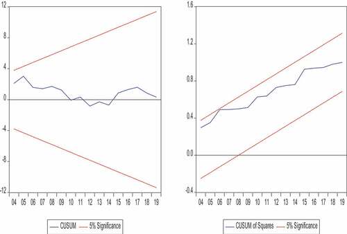
Lastly, the stability of the model for the long run and short-run relationship is detected by using the cumulative sum of recursive residuals (CUSUM) and the cumulative sum of squares of recursive residuals (CUSUMSQ) tests as proposed by (Brown et al., 1975). The pair of two straight lines that parallel in the following two graphs indicate the 5 percent significant level, and if the plotted CUMSUM and CUMSUMSQ graphs remain inside the straight lines then the null hypothesis of a correct specification of the model can be accepted. The two plots disclose that the plots of CUMSUM and CUMSUMSQ stay within the lines, and, therefore, this confirms the equation is correctly specified and the model is stable. Examination of the plots in Figure 2 shows that CUSUM and CUSUMSQ statistics are well within the 5% critical bounds implying that short-run and long-run coefficients in the ARDL models are stable.

Figure 2. Stability test.

4.4. ARDL bounds test result for co-integration

If the estimated F-statistics (13.57) value is greater than the upper-lower bound critical value, the null hypothesis of no co-integration must be rejected. This implies that the variables in the model share long-run relationships among themselves. From Table 4, it is clear that there is a long-run relationship amongst the variables.

Table 4. Co-integration test

F-Bounds Test	Value	Null Hypothesis: No levels relationship
F-statistic	13.57	10%	Lower	Upper
			2.45	3.52
Number of regressors	4	5%	2.86	4.01
		2.5%	3.25	4.49
		1%	3.74	5.06

4.5. Co-integration result: long run relationship of variables

Table 5 shows Ethiopia’s inflation rate in relation to long-run sectoral growth (services, industry, and agricultural sector) and population growth. In the agriculture sector, the elasticity is −21.59, in the service sector it is −21.53, in the industry sector it is 0.62, and in the population sector, it is −2.68. All variables except the industry sector play a significant role in reducing inflation in Ethiopia. Agriculture ranks first among economic sectors for reducing inflation, followed by the service sector.

Table 5. ARDL long relationship

Levels Equation (Case 3: Unrestricted Constant and No Trend): Dependent variables is LnINFR
Variable	Coefficient	Std. Error	t-Statistic	Prob.
LnAS	−21.59	4.880480	−4.423770	0.0004
LnIS	0.62	1.174693	0.532137	0.6019
LnSS	−21.53	5.287591	−4.071879	0.0009
LnPOP	−2.68	0.757104	−3.548696	0.0027

The agriculture sector is considered to be a driver of poverty reduction, employment creation, and export earnings in Ethiopia. Over the past decade, the agriculture sector has accounted for 50% of GDP, employed 85% of the labor force, and accounted for 90% of foreign exchange (NBE, 2015; NPC, 2016). When compared to the service and industry sectors, the sector continues to be the top source of employment. In addition, the agriculture sector has been shown empirically to contribute to Ethiopia’s economy and reduce inflation. As a result, the agricultural sector is expected to respond to rising demand with a flexible supply and, therefore, not experience inflationary pressure. Over the study period, the percentage contribution of agriculture to GDP has decreased, but this doesn’t mean the agricultural sector is losing relevance. Secondly, the services sector includes activities ranging from the production of goods to the distribution of them to consumers. It differs from Emeru (2020), but it’s consistent with Melaku (2020), when economic growth reduced inflation.

In recent years, the service sector has become the largest sector of the economy, moving away from the primary and secondary sectors. Ethiopia’s service and agricultural sectors contribute to economic growth in part because they compete with one another; the sectors also contribute to reducing inflation by propelling economic growth. According to statistical observations, the industry sector contributes to economic growth. The contribution is less than that of the service and agriculture sectors, but its contribution to reducing the inflation rate by increasing economic growth is insignificant. This study is consistent with Melaku (2020) because the service sector is part of economic growth.

According to this empirical investigation, population growth has been a contributing factor to reducing the inflation rate in Ethiopia. Other things being equal, the change in population growth causes the long-run inflation rate reduction to change by about 2. 68. The result does not fit Malthus’s theory; however, it does fit the theory of optimists. Petersen (1959), the rapid growth of the population in developing countries leads to social expenditures on education and health. A positive effect of population growth on economic growth was implied by the optimism theories, as human ingenuity would be sufficient to overcome environmental constraints. Because of Africa’s natural resources and fertile soil, population growth is not likely to pose a problem for that continent (Bogue, 1982).

Ethiopia is not a country with a high mass consumption level. However, Rostow (1960) shows that population growth is associated with a high level of consumption. His stages of economic growth show that the net investment rate increased along with the growth of the population. As a result, the increase in effective demand for their products contributed to the development of key sectors. Additionally, it contributed to increased entrepreneurial activity, leading to a reduction in inflation. As the population grows, the domestic market expands. This becomes increasingly relevant in the context of international competition, which in turn creates a more secure foundation for national production to grow and productivity to rise. In addition, the economies of scale-up, as well as the growth in the division of labor, also require a minimal investment in education and training per person. These factors can be particularly valuable for building a stock of useful knowledge. If more people are involved in creating this stock of knowledge, productivity will increase per capita.

4.6. Error correction regression: short run result

Table 6 shows that almost all coefficients are significant in their lags. The constant value, which describes the inflation intercept, is 651. The slope of a regression line can be explained by the value of a constant in a model. R-squared shows that the variable mentioned above has an influence, which results in 96%, and the remaining 4% is due to other variables not included in the model. Probability result of Breusch-Pagan-Godfrey test is 0.8611, meaning this high R-square is not the result of heteroscedasticity. Generally speaking, the results indicate an F-statistic of 18.41 with a probability of 0.000000, which indicates that the combined effect of the independent variables (services, agriculture, industry, and population growth) is statistically significant.

Table 6. ARDL error correction regression

Independent Variable	Dependent Variable: D(LNINF)
	Selected Model: ARDL(3, 5, 1, 5, 3)
	Case 3: Unrestricted Constant and No Trend
	Coefficient	Std. Error	t-Statistic		Prob.
C	650.9720	70.72285	9.204550		0.0000
D(LnINF(−1))	1.796098	0.298266	6.021804		0.0000
D(LnINF(−2))	0.623960	0.156087	3.997526		0.0010
D(LnAS_GDP_)	44.84324	14.95877	2.997789		0.0085
D(LnAS_GDP_(−1))	116.8607	17.49094	6.681215		0.0000
D(LnAS_GDP_(−2))	133.3126	16.05830	8.301786		0.0000
D(LnAS_GDP_(−3))	115.7252	19.86711	5.824960		0.0000
D(LnAS_GDP_(−4))	92.35328	18.05329	5.115593		0.0001
D(LnIS_GDP_)	−10.40165	3.491593	−2.979055		0.0089
D(LnSS_GDP_)	44.56318	10.74464	4.147480		0.0008
D(LnSS_GDP_(−1))	96.16745	15.08237	6.376150		0.0000
D(LnSS_GDP_(−2))	113.2419	13.89463	8.150048		0.0000
D(LnSS_GDP_(−3))	111.4946	18.33783	6.080032		0.0000
D(LnSS_GDP_(−4))	73.54451	15.54344	4.731546		0.0002
D(LnPOP)	−2.189247	15.79977	−0.138562		0.8915
D(LnPOP(−1))	−49.36493	21.74652	−2.270016		0.0374
D(LnPOP(−2))	25.42300	10.02251	2.536589		0.0220
CointEq(−1)*	−3.835257	0.416371	−9.211161		0.0000
R-squared (0.96)	Adjusted R-squared (0.89)			F-statistic (18.41), Prob (0.000000)

In Ethiopia, the current inflation rate is the result of previous inflation. Currently, strong inflation adaptation seems to serve as an effective inflation immobilizer, fueling continuous price-price spirals. Efforts to control inflation may be rendered ineffective. Ethiopia’s agricultural sector and its service sector have failed to reduce the inflation rate, as both have increased it. The industrial sector has effectively reduced inflation compared to the previous inflation rate, the second lag of population growth, agriculture, and the service sector. In the process of industrialization, resources move from agriculture to industry. An agricultural sector that is stagnant will lead to a growing demand for agricultural products and a decreasing supply in agriculture. Increasing demand for agricultural products results in higher prices due to the rigidity of supply and the inadequacy of export purchasing power, which prevents enough food imports. It is inconsistent with Melaku (2020).

In these circumstances, the ECT term has a negative value and is greater than one, resulting in 383% of sectoral growth convergent to its long-run equilibrium. The speed of adjustment to its long-run equilibrium is very fast as it takes only a few days for the model to fully adjust to its long-run equilibrium if shocks are introduced. R.E.A. Khan and Hye (2010) affirm that a very high speed of adjustment from short-run oscillation to long-run equilibrium (ECM coefficient is −2.01, showing a 201% correction per year). Moreover, it is also in line with (Birhanu et al., 2016; Munir et al., 2013; Fatimah & Anwarul, 2010) which shows that the disequilibrium of earlier period shocks will quickly adjust to the long-run equilibrium.

4.7. Pairwise Granger Causality Tests

In Table 7, it can be seen that the null hypothesis that LnAS does not Granger to LnINF is rejected; similarly, its counterpart that LnLNF does not Granger to LnAS is also rejected. Accordingly, the result indicates bidirectional causality between inflation and the agricultural sector. In the case of LnIS, the null hypothesis that states LnIS does not contribute to LnINF is rejected in favor of its alternative. In contrast, the null hypothesis that states LnINF does not contribute to LnIS is accepted. This tells us that there is unidirectional causality flowing from LnIS to LnINF. As for causality running from LnSS to LnINF, the null hypothesis is rejected as LnSS causes LnINF, its counterpart is false. There is causality from population to inflation but not vice versa. For causality running from LnIS to LnAS and LnAS to LnIS, the null hypothesis is rejected which means there is bidirectional causality between industry and agriculture sector. For the case of LnSS to LnAS, causality extending from LnSS to LnAS was found to be one-way. Likewise, unidirectional causality runs from LnAS to LnPOP, LnSS to LnIS and LnSS to LnPOP, so the null hypothesis is rejected. For the cases of other causality, the null hypothesis is accepted. Based on Degu (2019), the long run causality extends from the agricultural and service sectors to the industrial sector. According to the short run Granger causality results, the industrial and agricultural sectors are bi-directionally causal.

Table 7. Granger Causality test result

Null Hypothesis:	F-Statistic	Probability
LnAS does not Granger Cause LnINF LnINF does not Granger Cause LnAS	5.79223 2.63945	0.0065** 0.0647***
LnIS does not Granger Cause LnINF LnINF does not Granger Cause LnIS	6.35635 1.76832	0.0015* 0.1712
LnSS does not Granger Cause LnINF LnINF does not Granger Cause LnSS	3.13651 1.65373	0.0376 0.1948
LnPOP does not Granger Cause LnINF LnINF does not Granger Cause LnPOP	4.45874 0.32058	0.0125** 0.8104
LnIS does not Granger Cause LnAS LnAS does not Granger Cause LnIS	4.59161 3.15953	0.0082* 0.0367*
LnSS does not Granger Cause LnAS LnAS does not Granger Cause LnSS	2.51982 0.86754	0.0739*** 0.4671
LnPOP does not Granger Cause LnAS LnAS does not Granger Cause LnPOP	2.02763 2.67475	0.1279 0.0622***
LnSS does not Granger Cause LnIS LnIS does not Granger Cause LnSS	5.04667 0.26801	0.0052* 0.8480
LnPOP does not Granger Cause LnIS LnIS does not Granger Cause LnPOP	0.57667 0.15217	0.6342 0.9276
LnPOP does not Granger Cause LnSS LnGSS does not Granger Cause LnPOP	0.42663 4.29661	0.7351 0.0161**

*, ** and *** indicates the significance level of causality at 1%, 5% and 10%

5. Conclusion and policy implication

The purpose of this study was to evaluate the associations between inflation rate and service, agriculture, and industry sector, as well as population growth in Ethiopia from 1975–2019. We find that population growth, services, and the agricultural sector have contributed to reducing inflation in the long run. However, the industry sector reduces inflation in the short run, even though it has no contribution to reducing inflation in the long run. The first and second lags of inflation rates, the service sector, the second lag of population growth, and agriculture up to four lags have a positive effect on inflation in the short run. Considering the long-term negative effects of the service sector, Ethiopia can lower its inflation rate by raising the service sector like financial services industry, internet technology, hotels, real estate, education, health, social work, media, communications, electricity, tourism, gas and water supply. In this sense, the service sector in Ethiopia can play a more significant role in reducing inflation and will empower the overall economy of the country. Expand the profitable service sector, ensure that supply and demand in the service sectors are in balance, and use advanced technology to increase the productivity of service sectors.

In the long run, agriculture can reduce inflation. Agricultural growth is more effective at raising incomes and reducing inflation among the poor. More than 35% of the gross domestic product (GDP) is accounted for by it. In order to leverage unused arable land, modernize production systems, and improve technology adoption. In the same way, the government should prioritize irrigation development on a small and large scale, and financing agricultural inputs. The industrial sector, serve as important sources of employment, especially for the rapidly growing urban population. Taking this into account, its contribution to reducing inflation rate is insignificant, in the long run, but in the short run, it does play a significant role in reducing inflation.

To address the large population growth interest and to reduce inflation in the country, the Ethiopian government should develop human resource deployment, expand industrial sectors, introduce education for self-reliance, develop funds supporting the development of women and youth, expand vocational education and training, strengthen agriculture policy, transfer of know-how, increase partnership between public and private sectors, create labor-intensive projects, and expand key economic infrastructure. Furthermore, the government should consolidate the existing entrepreneurship activity and attract new entrants to the field in order to create more jobs and absorb a large number of unemployed people. Those conditions aid the government in reducing unemployment from high population growth.

6. Insight for further studies

The current study is based on countrywide sectoral growth as a proxy for economic growth on the inflation rate. Researchers in this area may also consider using panel data to compare the sectoral responsibility for reducing inflation in other African countries.

Disclosure statement

No potential conflict of interest was reported by the author(s).

Additional information

Funding

For this research, the authors did not receive any funding.

Notes on contributors

Endashaw Sisay

Endashaw Sisay holds Master of Science in economics from Jimma University. Now he is lecturer at Mizan Tepi University, department of economics. His research interests include, financial economics, econometrics and industrial economics.

Wondimhunegn Atilaw

Wondimhunegn Atilaw holds Master of Science in economics from Jimma University. Now he is lecturer at Mizan Tepi University, department of Economics. His research interests include financial economics, macroeconomics and environmental economics.

Tecklebirhan Adisu

Tecklebirhan Adisu got his Masters of Science in Marketing Management from Bahirdar University. Now he is lecturer at Mizan Tepi University, department of Marketing Management. His research focuses on consumer behavior, profitability of companies and society welfare.

References

- Afzal, M., Malik, M. E., Butt, A. R., & Fatima, K. (2013). Openness, inflation and growth relationships in Pakistan an application of ARDL bounds testing approach. Pakistan Economic and Social Review, 51(1), 13–24.
- Alemu, M., Mulugeta, W., & Wassie, Y. (2016). Monetary policy and inflation dynamics in Ethiopia: An empirical analysis. Global Journal of Human-Social Science: E Economics, 16(4 45–60).
- Alemu, Z. G., Oosthuizen, K., & Schalkwyk, H. D. 2003. Contribution of agriculture in the Ethiopian economy: A time-varying parameter. Approach. Agrekon. 42 1 29–48 doi:10.22004/ag.econ.246011. 1.
- Argy, V. (1970). Structural inflation in developing countries. Oxford Economic Papers, 22(1), 73–85. https://doi.org/10.1093/oxfordjournals.oep.a041153
- Arltová, M., & Fedorová, D. (2016). Selection of unit root test on the basis of time series length and value of ar(1) parameter. Statistika: Statistics and Economy Journal, 96(3), 47–64 http://www.czso.cz/statistika_journal .
- Ayyoub, M. (2015). Inflation and sectoral growth in developing economies. In PhD Dissertation, Innsbruck. University of Innsbruck 29 .
- Bane, J. (2018). Dynamics and determinants of inflation in Ethiopia. perspectives on development. the Middle East and North Africa (MENA) Region, 67–84 doi:10.1007/978-981-10-8126-2_4.
- Bekhet, H. A., & Al-Smadi, R. W. (2015). Determinants of Jordanian foreign direct investment inflows: Bounds testing approach. Economic Modeling, 46 C , 27–35. https://doi.org/10.1016/j.econmod.2014.12.027
- Birhanu, B., Mulugeta, W., & Yaekob, T. (2016). Relationship between government revenue growth and economic growth in Ethiopia. International Journal of Research in Computer Application and Management, 6(8 47–55 https://www.researchgate.net/publication/315045775_RELATIONSHIP_BETWEEN_GOVERNMENT_REVENUE_GROWTH_AND_ECONOMIC_GROWTH_IN_ETHIOPIA).
- Block, S. A. (1999). Agriculture and economic growth in Ethiopia: Growth multipliers from a four- sector simulation model. Agricultural Economics, 20, 241–252 file:///C:/Users/user/Downloads/agec1999v020i003a005.pdf.
- Bogue, D. J. (1982). Review of population and technological change: A study of long-term trends. By E. Boserup. American Journal of Sociology, 88(2), 461–463. https://doi.org/10.1086/227695
- Brown, R. L., Durbin, J., & Evans, J. M. (1975). Techniques for testing the constancy of regression relationships over time. Journal of the Royal Statistical Society, Series B (Methodological), 37(2), 149–192 https://rss.onlinelibrary.wiley.com/doi/10.1111/j.2517-6161.1975.tb01532.x.
- Busse, M., & Hefeker, C. (2007). Political risk, institutions and foreign direct investment. European Journal of Political Economy, 23(2), 397–415. https://doi.org/10.1016/j.ejpoleco.2006.02.003
- Canavese, A. J. (1982). The structuralism explanation in the theory of inflation. World Development, 10(7), 523–529 https://doi.org/10.1016/0305-750X(82)90053-5.
- Chaudhry, I. S., Ayyoub, M., & Imran, F. (2013). Does inflation matter for sectoral growth in Pakistan? An empirical analysis. Pakistan Economic and Social Review, 51(1 71–92 https://www.semanticscholar.org/paper/DOES-INFLATION-MATTER-FOR-SECTORAL-GROWTH-IN-An-Chaudhry-Ayyoub/56cb732e504be176eb2fe720116d9d982fe48f27).
- Chewaka, J. E. (2014). Comment: Legal aspects of stock market development in Ethiopia: Comments on challenges and prospects. Mizan Law Review, 8(2), 439–454. https://doi.org/10.4314/mlr.v8i2.7
- Clark, C. (1940). The conditions of economic progress. Macmillan. https://archive.org/details/in.ernet.dli.2015.223779
- CSA (2022). Country and regional level consumer price Indices’, Monthly report on consumer price index, various months.
- Degu, A. A. (2019). The causal linkage between agriculture, industry and service sectors in Ethiopian economy. American Journal of Theoretical and Applied Business, 5(3), 59–76. https://doi.org/10.11648/j.ajtab.20190503.13
- Denbel, F. S., Ayen, Y. W., & Regasa, T. A. (2016). The relationship between inflation, money supply and economic growth in Ethiopia: Co-integration and causality analysis. International Journal of Scientific and Research Publications, 6(1 556–565 https://www.ijsrp.org/research-paper-0116/ijsrp-p4987.pdf).
- Dickey, D. A., & Fuller, W. A. (1979). Distribution of the estimators for autoregressive time series with a unit root. Journal of the American Statistical Association, 74 366a , 427–431. https://doi.org/10.1080/01621459.1979.10482531
- Durguti, E., Tmava, Q., Demiri-Kunoviku, F., Krasniqi, E. . (2021). Panel estimating effects of macroeconomic determinants on inflation: Evidence of Western Balkan. Cogent Economics & Finance, 9(1 1–13). https://doi.org/10.1080/23322039.2021.1942601
- Emeru, G. M. (2020). The determinants of inflation in Ethiopia: A multivariate time series analysis. Journal of Economics and Sustainable Development, 11(21 53–62 https://pdfs.semanticscholar.org/2056/9dc1d27fffbf86e85c91b3f0849615d7c32c.pdf?_ga=2.217315990.1675148764.1663096923-1930156572.1624445562).
- Faridi, M. Z. (2012). Contribution of agricultural exports to economic growth in Pakistan. Pakistan Journal of Commerce and Social Sciences, 6(1), 133–146 https://www.econstor.eu/bitstream/10419/188047/1/pjcss079.pdf.
- Fatimah, M. A., & Anwarul, H. (2010). Supply response of potato in Bangladesh: A vector error correction approach. Journal of Applied Sciences, 10(11 895–902 http://scialert.net/abstract/?doi=jas.2010.895.902).
- Fisher, I. (1911). The equation of exchange, 1896-1910. American Economic Review.
- Fisher, G. B. A. (1935). The clash of progress and security. Macmillan.
- Friedman, M., & Schwartz, A. J. (1963). A monetary history of the United States, 1867- 1960. Princeton. The Princeton University Press.
- Getachew, Abis, & Meaza, Cherkos. (2018). Do prices influence economic growth? Estimating the inflation threshold of the Ethiopian economy. Journal of Economics and Sustainable Development, 9(1 46–56).
- Granger, C. W. (1969). Investigating causal relations by econometric models and cross-spectral methods. Econometrica, 37(3), 424–438. https://doi.org/10.2307/1912791
- Gujarati, D. N. (2004). Basic econometric (4th ed.). the McGraw-Hill Companies. NewYork.
- Harris, H., & Sollis, R. (2003). Applied time series modelling and forecasting. Wiley, West Sussex.
- Hume, D. (1752). Political discourses (Kessinger Publishing).
- Humphrey, T. M. (1998). Historical origins of the cost-push fallacy. Economic Quarterly, 84 3 , 53–74 https://www.richmondfed.org/-/media/RichmondFedOrg/publications/research/economic_quarterly/1998/summer/pdf/humphrey.pdf.
- Humuda, A.M, Sulikova, V., Gazda, V., & Horvath, D. (2013). ARDL investment model of Tunisia. Theoretical and Applied Economics, XX 2 , 57–68.
- Hussin, F., & Yik, S. Y. (2012). The contribution of economic sectors to economic growth: The cases of China and India. Research in Applied Economics, 4(4 38–53). https://doi.org/10.5296/rae.v4i4.2879
- Jaffri, A. A., Farooq, F., & Munir, F. (2016). Impact of demographic changes on inflation in Pakistan. Pakistan Economic and Social Review, 54(1), 1–14. https://www.jstor.org/stable/26616694
- Kahssay, T. (2017). Determinants of inflation in Ethiopia: A time-series analysis. Journal of Economics and Sustainable Development, 8(19 1–6 https://www.iiste.org/Journals/index.php/JEDS/article/view/39294/40403).
- Kaur, S. (2013). Inflation impact on Indian economy and agriculture. International Journal of Scientific & Engineering Research, 4(7 1459–1462).
- Kaur, R., & Aggarwal, P. K. (2019). The contribution of the service sector to economic growth in India. IOSR Journal of Economics and Finance, 10(3), 01–09 https://iosrjournals.org/iosr-jef/papers/Vol10-Issue3/Series-5/A1003050109.pdf.
- Keynes, J. M. (1936). The general theory of employment, interest, and money. Macmillan Publication.
- Khan, R. E. A., & Hye, Q. M. A. (2010). Financial sector reforms and household savings in Pakistan: An ARDL approach. African Journal of Business Management, 4(16), 3447–3456.
- Khan, A. H., & Qasim, M. A. Inflation in Pakistan revisited. (1996). Pakistan Development Review, 35(4), 747–759. Part II:. https://doi.org/10.30541/v35i4IIpp.747-759
- Lewis, A. W. (1954). Economic development with unlimited supply of labor. the manchester school. In A. N. Agrawal & S. P. Singh (Eds.), The economics of under- development (Reprinted in (John Wiley & Sons, Inc) ed.) (pp. 400–449).
- Liew, V. K. (2004). Which lag length selection criteria should we employ? Economics Bulletin, 3 33 , 1–9.
- Lim, Y. C., & Sek Siok, K. (2015). An examination on the determinants of inflation. Journal of Economics, Business and Management, 3(7), 678–682. https://doi.org/10.7763/JOEBM.2015.V3.265
- Lindh, T., & Malmberg, B. (2000). Can age structure forecast inflation trends? Journal of Economics and Business, 52(1–2), 31–49. https://doi.org/10.1016/S0148-6195(99)00026-0
- Loening, L. J., Durevall, D., & Birru, Y. A. (2009). Inflation dynamics and food prices in an agricultural economy: The case of Ethiopia. Working Paper 347. Gothenburg: University of Gothenburg.
- Loto, M. A. (2012). Global economic downturn and the manufacturing sector performance in the Nigerian economy (A quarterly empirical analysis). Journal of Emerging Trends in Economics and Management Sciences, 3(1), 38–45.
- Lucas, R. E. (1972). Expectations and the neutrality of money. Journal of Economic Theory, 4(2), 103–124. https://doi.org/10.1016/0022-0531(72)90142-1
- Malthus, T. R. (1798). An essay on the principle of population. J. Johnson.
- McCallum, B. T. (1980). Rational expectations and macroeconomic stabilization policy: An overview. Journal of Money, Credit, and Banking, 12(4), 716–746. https://doi.org/10.2307/1992031
- Mekonen, E. K. (2020). Agriculture sector growth and inflation in Ethiopia: Evidence from autoregressive distributed lag model. Open Journal of Business and Management, 8(6), 2355–2370. https://doi.org/10.4236/ojbm.2020.86145
- Melaku, M. (2020). Determinants of inflation in Ethiopia. Academic Journal of Research and Scientific Publishing, 2(18 68–88).
- Mkhatshwa, Z. S., Tijani, A. A., & Masuk, M. B. (2015). Analysis of the relationship between inflation, economic growth and agricultural growth in Swaziland from 1980-2013. Journal of Economics and Sustainable Development, 6 18 , 189–204.
- Munir, S., Kiani, A. K., Khan, A., & Jamal, A. (2013). The relationship between trade openness and income inequalities empirical evidences from Pakistan (1972-2008). Academic Journal of Management Sciences, 2(1), 21–35.
- Nawaz, M., Naeem, M., Ullah, S., & Khan, S. U. (2017). Correlation and causality between inflation and selected macroeconomic variables: Empirical evidence from Pakistan (1990-2012). iBusiness, 9(4), 149–166. https://doi.org/10.4236/ib.2017.94011
- NBE. (2015). National Bank of Ethiopia annual report on Ethiopian economy: Addis Ababa.
- NBE. (2017). National Bank of Ethiopia annual report on Ethiopian economy: Addis Ababa.
- NBE. (2019). National Bank of Ethiopia annual report on Ethiopian economy: Addis Ababa.
- Ndour, C. T. (2017). Effects of human capital on agricultural productivity in Senegal. World Scientific News, 64, 34–43.
- Ng, S., & Perron, P. (2001). LAG length selection and the construction of unit root tests with good size and power. Econometrica, 69(6), 1519–1554. https://doi.org/10.1111/14680262.00256
- NPC. (2016) . Growth and transformation Plan-II of Ethiopia. volume I main text. Addis Ababa.
- Okun, A. M. (1962). Potential GNP & its measurement and significance, American statistical association. Proceedings of the business and economics statistics section, pp. 98–104.
- Olaniyi, O. Z., Mathew, A., Ogunleye, A. A., & Oladokun, Y. O. M. (2015). An empirical analysis of the contribution of agricultural sector to Nigerian gross domestic product: Implications for economic development. Developing Country Studies, 5(21).
- Olivera, J. H. (1964). On structural inflation and Latin-American’ structuralism. Oxford economic papers 16 3 , pp. 321–332 https://doi.org/10.1093/oxfordjournals.oep.a040958.
- Omoniyi, L. G., & Olawale, A. N. (2015). An application of ARDL ounds testing procedure to the estimation of level relationship between exchange rate,crude oil price and inflation rate in Nigeria. International Journal of Statistics and Applications, 5, 81–90.
- Oyakhilomen, O., & Rekwot, Z. G. (2014). The relationships of inflationary trend, agricultural productivity and economic growth in Nigeria. CBN Journal of Applied Statistics, 5 1 35–47 .
- Pesaran, M. H., Shin, Y., & Richard, J. S. (2001). Bounds testing Approaches to the analysis of level relationships. Journal of Applied Econometrics, 16(3), 289–326. https://doi.org/10.1002/jae.616
- Pesaran, M. H., Shin, Y., & Smith, R. P. (1999). Pooled mean group estimation of dynamic heterogeneous panels. J. Am. Stat. Assoc, 94(446), 621–634. https://doi.org/10.1080/01621459.1999.10474156
- Petersen, W. (1959). Population growth and economic development in low-income countries: A case study of India’s prospects. In B. A. J. Coale & G. M. Hoover. eds., The Journal of Asian Studies. Princeton University Press. xxi, 389. $8.50. Vol. 18. 524–525. https://doi.org/10.2307/2941169.
- Phillips, A. W. (1958). The relation between unemployment and the rate of change of money wage rates in the United Kingdom, 1861-1957. Economica, 25(100), 283–299. https://doi.org/10.1111/j.1468-0335.1958.tb00003.x
- Rostow, W. W. (1960). The stages of economic growth: A non-communist manifesto. Cambridge University Press.
- Sargent, T. J., & Hansen, L. P. (1980). Formulation and estimating dynamic linear rational expectations models. Journal of Economic Dynamics & Control, 2(11), 7–46. https://doi.org/10.1016/0165-1889(80)90049-4
- Seleteng, M. (2013).Inflation and economic growth nexus in the Southern African Development Community: a panel data investigation (Doctoral dissertation, University of Pretoria).
- Sirah, E. S. (2020). Short run impact of public finance on inflation rate in Ethiopia; empirical evidence with time series analysis (1974/75-2018/19). Journal of Economics and Sustainable Development, 11(9 42–45).
- Sirah, E. S., Wtensay, W. A., & Shah, S. A. (2021). Impact of Africa growth and opportunity act and merchandise exports on the Ethiopian economy over the long term. Innovations 67 , (02 142–158).
- Sisay, E., Wassie, Y., & Alemu, M. (2020). Unemployment and the macroeconomics of Ethiopia. International Journal of Commerce and Finance, 6(2), 40–49.
- Tafere, K. (2008). The sources of the recent inflationary experience in Ethiopia. An MSc Thesis, Addis Ababa University.
- Ukpolo, V. (2002). Population growth and economic growth in Africa. Contributions to Asian Studies, 18(4), 315–329. https://doi.org/10.1177/0169796x0201800402
- Xinshen, D., & Steven, H. B. F. (2007). Agricultural growth linkages in Ethiopia: Estimates using fixed and flexible price models. Washington: International Food Policy.
- Yamaguchi, K. (2013). Money and macroeconomic dynamics (First ed.). Osaka Office Publications.
- Yismaw, T. G. (2019). Effect of inflation on economic growth of Ethiopia. Journal of Investment and Management, 8(2), 48–52. https://doi.org/10.11648/j.jim.20190802.13
- Zulfiqar, Z. (2015). Inflation, interest rate and firms’ performance: The evidences from textile industry of Pakistan. International Journal of Arts and Commerce, 4(2 111–115).