Impacts Of Fishing On The Rural Household Income; Evidence From Ethiopian Rift-Valley

Abstract

Fish farming is a vital resource to fight poverty and food insecurity through the diversification of income sources. However, little has been investigated on its actual contributions to increase household income. This study envisages the impacts of fishing on the household income in Lume District, Ethiopian Rift valley. The quasi-experimental research design was used. Both qualitative and quantitative data were collected from both primary and secondary sources. Two-stage stratified sampling procedures were employed and about 374 sample households (about 202 non-fishing and 172 fishing households) were randomly selected. Structured interview schedules, key informant interviews, and focused group discussions were employed to collect the relevant data. Descriptive statistics (frequency, percentage, mean, and standard deviation) and the Propensity score matching method were employed to analyze the data. STATA V.13 software was used as an analytical tool. Fishing and non-fishing households had earned an annual income of about 36,914.85 and 31,768.43 Ethiopian Birr per year respectively. The model output reveals that the average treatment effect on the treated is about ETB 5146.42 and the mean difference in the average effect of the treatment on the treated between the matched treatment and control groups was found to be statistically significant at a 5% significance level. Overall, participation in fishing has generated about a 7.5% increase in farm annual income of treated households over control groups. It can be concluded that participation in fishing has brought a positive and significant impact on improving a household’s annual income status in the study area. Therefore, special attention should be given by governmental and non-governmental organizations to improve the fish and aquaculture sector in the area through the introduction and dissemination of innovations that can enhance fish productivity in the study area.

Keywords:

• Ethiopia
• fish production
• income
• propensity score matching

1. Introduction

Fish is an aquatic animal that serves as the source of food, nutrition, income, and livelihood for millions of people in the world (Food and Agriculture Organization (FAO), 2018). Fishing is animal-based food production that has quickly grown sector since the ancient civilization of Egypt and China (Amare et al., 2018). Nowadays, it is practiced both in developed and developing countries with different production statuses through both capture and aquaculture fisheries. From global fish production of 171 million tons, capture fisheries represented about 90.63 million tons, which cover 53% of the total fish production (Food and Agriculture Organization (FAO), 2018).

In developing countries, the livelihood of more than 500 million people is directly or indirectly tied to fisheries (FAO, 2020). Historically, Africa’s fisheries are increasingly contributing to food and nutrition security, foreign exchange, employment, and livelihood support services (De Graaf & Garibaldi, 2019). The New Partnership for Africa’s Development (NEPAD) estimates that total fishery production in the region stands at 10.4 million tons (NEPAD, 2014 as cited in Gatriay Tut Deng, 2020) comprising 6.0 million tons from marine capture fisheries, 2.8 million tons from inland water fisheries, and about 1.6 million tons from aquaculture.

In the content, about 12.3 million people work in the fisheries sector, with 6.1 million (50%) being employed as fishers, 5.3 million (42%) as processors, and 0.9 million (8%) as fish farmers (De Graaf & Garibaldi, 2019). In terms of economic value, fish produces an estimated total of US$24 billion annually, accounting for 1.26% of gross domestic product (GDP) (NEPAD, 2014 as cited in Gatriay Tut Deng, 2020). As compared to the marine fishery, inland fisheries of Africa have 2.1 million tons of fish which has become a major export item for Africa with an annual export value of $2.7 billion (Tilahun et al., 2018).

Ethiopia is a landlocked country and depends on its inland waterbodies for fish supply for its population which has a great value in socio-economic, ecological, and scientific aspects (Amare et al., 2018). The country is known for being the water tower of Eastern Africa, encompassing about waterbodies of 7334-kilo meter square (KM²) of the lake area and a total river length of 7000 km² have a huge potential for fisheries production (Food and Agriculture Organization (FAO), 2018). Ethiopia’s capture fishery locations consist of: the Great Rift Valley lakes, Lake Tana, numerous rivers, and minor waterbodies, including reservoirs and natural impoundments (FAO, 2020). According to Assefa and Abebe (2018), the commercial fishery is concentrated at Lakes Tana, Chamo, Ziway, Abaya, Koka, Langano, Hawassa, and the northern part of Turkana provides a higher fish supply to the major urban center in Ethiopia. Those diverse waterbodies support diverse aquatic life including more than 180 fish species

The Fisheries sector is underutilized particularly, commercialization of fisheries was given limited focus. When the sector is recognized and supported with adequate strategies and policy it can play a significant role in overall rural economy development (Food and Agriculture Organization (FAO), 2018). According to the Ethiopia Ministry of Agriculture (MoA, 2020), the fisheries subsector is one of the potential intervention areas to achieve the objective of enhancing food security, employment, and providing a source of income to improve the livelihood of rural people sustainably. Primarily it serves as income generation which is ultimately used for the purchase of a variety of food and non-food items (Tilahun et al., 2018).

In the Lume district, Lake Koka fisheries have been developing over the past decades and the lake was part of the major lakes considered by the lake fisheries development project (LDP) in the 1990s (Lume District office of Agriculture, 2020). It has a huge fish potential to produce 1194 tons per year and is one of the freshwater bodies where the commercial fishery is focused that used many rural households as its main income source. The Lake is dominated by commercially important consumable fish species; such as Nile tilapia (Oreochromis niloticus), Common carp (Cyprinus carpio), and Catfish (Clarias gariepinus). It is an open and easily accessible resource that is the most important lake to all adjacent districts for 15,000 local people who have been directly relying on the lake (Endalew et al., 2020).

The research that highlights the relationships between fishery production and income and the role of fisheries in local food security and poverty reduction are critically important for policy development that sustainably supports the sector. However, the primary attention of many studies was on the description of the waterbodies and limnological features of lakes and reservoirs, the biology of fish species, stock assessment of fishery, the composition of commercially important fish species and fisheries baseline information among the others (Alemayehu Abebe Wake and Tamiru Chalchisa Geleto, 2019; Endalew et al., 2020). Therefore, this study was conducted to analyze the impacts of fishing on the rural household’s income considering the current debate on the roles of the fisheries sector in poverty alleviation through income diversification in Lume District, Ethiopian Rift valley.

2. Literature review

In Ethiopia from 1940 and 50, the rapid population growth, which resulted in a shortage of cultivable land and depletion of land resources, forced the people to look for other occupations and sources of food from water resources at a subsistence level. The rapidly growing demand for fish in the capital city by foreigners and modern town-dwellers contributed to the start of commercial fishing as a new practice in Rift Valley lakes (from the 1950s) and, later, in Lake Tana late 1980s (Ayalew et al., 2018). Mostly in the country types of fish production are dominated by artisanal fisheries which are traditional that involve fishing households using a relatively small amount of capital and energy, relatively small fishing vessels, making short fishing trips, close to shore, mainly for local consumption (Food and Agriculture Organization (FAO), 2018). Many people usually use multi-target and a range of gears and vessels, which are having low capital, invest and perform activities along the coast.

Most fish product sources are fishery cooperatives from different lakes and reservoirs, street traders and brokers, fish shops, hotels, and restaurants (Assefa, 2013). Fresh fish is mostly collected in the area of the Great Rift Valley lakes and around Lake Tana. Besides, outside of these areas, the domestic fish market is insignificant. Form different species, Oreochromis niloticus (Nile Tilapia) is one of the most important species that is highly produced in capture fishery and aquaculture in more than 100 countries. Similarly, in Ethiopian fisher, Nile Tilapiais predominantly targeted and the leading species caught and consumed in most fishery production areas (Vijverberg et al., 2012).

In all fishing areas, its production activities are done during the morning, day, and night time in all seasons. Fish production status in Ethiopia is based on the principle of open access to resources that are characterized by different fishing gears. In the fish production system fishing gear technology commonly functioned in Ethiopian fisheries includes gillnets, beach seines, long-lines, hook-and-line, and cast nets (Brook, 2012). In addition to this, different forms of traps, scoop nets, and baskets made of plant materials and wires are also used, particularly in the rivers of Ethiopia.

In all production areas, most of the fish caught from the lakes reach the market by traditional means of transportation without any preservation facilities (Brook, 2012). Some fishermen hook some of the fish together with a string and carry them by hand to the market for immediate cash income. Others put the fish in a basket, cover them with fresh leaves and carry them by hand. Still, others collect their catch in sacks and carry it to the market by hand or on donkeys, taxis, or Pickup trucks. The most common forms of fish storage are the use of deep freezers of varying sizes and cold rooms in some cases at Arba Minch, Bahir Dar, Ziway, and Addis Ababa.

The riverine fishery is not developed due to a lack of access to suitable fishing grounds and also the food habit or culture of most of the rural community which does not favor fish consumption. Its fishing activities are performed mostly on two rivers, the Baro near Gambela in the Western part of the country (Husien et al., 2016) and the Omo in the Southern area near the border with Kenya. Fishing is done mainly with hooks and some gill nets. According to Alemu et al. (2014) report, the fishery production systems in five different rivers, namely, Ganale, Awata, and Dawa (Guji zone) and Gidabo and Galana (Borana zone) are characterized as agro-pastoral systems with the absence of efficient fishing and production system. Related to its marketing system, the produced fish size and type of fish play an important role in the cost and price in the market.

3. Methods

3.1. Description of the study area

The study was conducted in Oromia Region, East showa Zone of Lume district of three Kebeles namely: Koka Negawo, Derar Dembela, and Dungugi Bekele (Figure 1). The district is located 74 km South-East of Addis Ababa and 27 km from Bishoftu. Lume is bordered by Lake Koka on the south, Ada’a Chukala on the west, Gimbichu on the North West by, Amhara Region on the north, and the east by Adama. Mojo is the capital of the district (Lume District office of Agriculture, 2020).

Figure 1. Map of the study area Source: Arc GIS.

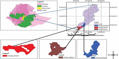
The total population of the Lume district is 117,415 of which 75,310 (44,472 males and 30,838 females) live in rural areas while 42,405 (20,570 male and 21,835 female) live in urban areas. The district is characterized by a subsistence mixed farming system in which both crops and livestock were kept together. Additionally, fishing and irrigation activities are common economic activities.

Koka dam is found on the Awash River in East Shewa Zone, 75 km South-east of Addis Ababa (BirdLife International, 2022). The lake mainly serves the local communities through fishing, watering for the animals, small and mechanized large irrigation farms (Lume District office of Agriculture, 2020).

3.2. Research design

As a strategy, the quasi-experimental research design was employed. This study used both primary and secondary data sources which are quantitative and qualitative.

3.3. Sampling procedure and sample size determinations

The study employed a two-stage stratified sampling procedure. In the first stage, Lume distract three Kebeles, namely; Koka Negawo, Derar Dembela, and Dungugi Bekele were selected purposefully based on their proximity to the main waterbody; Lake Koka.

In the second stage, households in the Kebeles were stratified into fishing and non-fishing households. From the first strata fishing household, the study used the farmers who are using fish as their sources of livelihood for three years or more as inclusion criteria. From the other stratum, non-fishing households (who were not engaged in fishing as a source of their income) were selected. Finally, about 374 sample households were identified through a simple random sampling technique. Population proportion samples were used to redistribute samples across all kebeles. Kothari’s (2004) formula was used to determine the sample size. When the population size is finite, the formula for sample size determination was used as:

(1) $n=\frac{Z^2.p.q.N}{e^2\left(N-1\right)+Z^2.p.q}$(1)

where n = sample size z = the value of standard variant at a given confidence level and to be worked out from the table showing area under the normal curve (z = 1.96 at 95% level of precision)

p = sample proportion (0.5) q = 1-p (1–0.5 = 0.5)

e = acceptable error (5% or 0.05) N = Number of total household (14,576)

Then, sample size will be reduced by taking total population of farmers in the district

$n=\frac{{\left(1.96\right)}^2\left(0.5\right)\left(0.5\right)\left(14,576\right)}{{\left(0.05\right)}^2\left(14,576-1\right)+{\left(1.96\right)}^{\left(2\right)}\left(0.5\right)\left(0.5\right)}n=374$

Of the population, 172 fishing households and 202 non-fishing households were selected in simple random techniques to provide an equal chance for the entire participants. The selected respondents from each kebeles are described in Table 1 below.

Table 1. Respondent household sampled from each selected Kebele

Location	Fishing households (N = 172)			Non-fishing households (N = 202)			Total sample size
	Total HH	Percent Weight	Sample Size	Total HH	Percent weight	Sample Size
Koka Nagawo Kebele	89	29	50	123	12	24	74
Derar Denbela Kebele	97	31	53	290	30	61	114
Dungugi Bekele	126	40	69	569	58	117	186
Total	312	100	172	982	100	202	374

Source: (Lume District office of Agriculture, 2020)

3.4. Methods of data collection

To achieve the objectives of the study, structured interview schedules, key informant interviews, and focus group discussions were used to collect both quantitative and qualitative data. Primary data were collected from a total of 374 household heads, 8 key informants, and 3 focus group discussants. The number of key informants and focused group discussants were determined based on data saturation theory. Before conducting the actual survey, the pilot test was conducted to check data collection instruments, and revision was made accordingly.

3.5. Methods of data analysis

Descriptive statistics and an econometric model were used to analyze the data by using STATA V.13. As descriptive statistics such as percentage, frequency, mean and standard deviation were employed. To evaluate the impact of fishing on household income, propensity score matching (PSM) was employed. In impact analysis, the PSM method is generally adopted in various literature (Ali & Erenstein, 2017; Gebrehiwot & Anne Van Der, 2015; Riehl et al., 2015). For this study, PSM was opted due to the unavailability of baseline data regarding household income. The specification of the PSM model was described below.

(2) $\mathrm{P}\left(\mathrm{X}\right)=\mathrm{P}\mathrm{r}\left\{\mathrm{D}=1/\mathrm{X}\right\}=\mathrm{E}\left\{\mathrm{D}/\mathrm{X}\right\}$(2)

Where D = {0¸1} is the indicator of exposure to treatment and (X) is the multidimensional vector of pretreatment characteristics. PSM constructs a statistical comparison group that is based on a model of the probability of participating in the treatment (T) conditional on observed characteristics (X), or the propensity score: P(X) = Pr (T = 1/X). Rosenbaum and Rubin (Rosenbaum & Rubin, 1983) showed that under certain assumptions, matching on P(X) is as good as matching on (X). The propensity score match approach tries to capture the effects of different observed covariates (X) on participation in a single propensity score or index. Then, outcomes of participating and non-participating households with similar propensity scores are compared to obtain the program effect. Households for which no match is found are dropped because no basis exists for comparison.

Matching aims to find the closest comparison group from a sample of non-participants to the sample of participants. “Closest” is measured in terms of observable characteristics not affected by program participation. The impact of treatment on the individual is the difference between potential outcomes with and without treatment in estimating the effect of a household’s participation in fishing which the outcome is specified as:

(3) $\delta \mathrm{\_}\mathrm{i}=\mathrm{Y}\mathrm{\_}1\mathrm{i}-\mathrm{Y}\mathrm{\_}0\mathrm{i}$(3)

Where, Y_1 = outcome of treatment (farm income of household when she/he does involve in fishing), Y_0 = Outcome of untreated individuals (farm income when he/she does not involve in fishing), and δ͟ i = Change in the outcome as a result of treatment or change of income for participating in fishing. To evaluate the impact of a program on the population, we might be computed the average treatment effect (ATE). The average treatment effect (ATE) could be computed as follows:

(4) $\mathrm{A}\mathrm{T}\mathrm{E}=\mathrm{E}\left[\delta \mathrm{i}\right]=\mathrm{E}\left(\mathrm{Y}\mathrm{i}-\mathrm{Y}0\right)$(4)

Most often, we were interested in computing the average treatment effect on the treated (ATT):

(5) $\mathrm{A}\mathrm{T}\mathrm{E}=\mathrm{E}\left(\mathrm{Y}1-\mathrm{Y}0/\mathrm{D}=1\right)$(5)

Where D = 1 refers to the treatment. The problem is that not all of these parameters are observable, as they rely on counterfactual outcomes. For instance, we could rewrite ATT as:

(6) $\mathrm{A}\mathrm{T}\mathrm{E}=\mathrm{E}\left(\mathrm{Y}1/\mathrm{D}=1\right)-\mathrm{E}\left(\mathrm{Y}0/\mathrm{D}=1\right)$(6)

The second term, E (Y₀ | D = 1) is the average outcome that the treated individuals would have obtained in absence of treatment, which is not observed. However, we do observe the term E(Y₀| D = 0) that is, the value of Y₀ for the untreated individuals.

(7) $\mathrm{A}\mathrm{T}\mathrm{T}=\mathrm{E}\left({\mathrm{Y}}_1|\mathrm{D}=1\right)-\mathrm{E}\left({\mathrm{Y}}_0|\mathrm{D}=0\right)$(7)

The second term is the average outcome of treated individuals had they not received the treatment. We couldn’t observe that, but we do observe a corresponding quantity for the untreated and could be computed given the assumption the PSM estimator of ATT:

(8) $\mathrm{A}\mathrm{T}\mathrm{T}=\mathrm{E}\left(\mathrm{Y}1-\mathrm{Y}0\hspace{0.17em}\mathrm{D}=0,\mathrm{p}\left(\mathrm{X}\right)\right)=\mathrm{E}\left(\mathrm{Y}1/\mathrm{D}=1,\mathrm{p}\left(\mathrm{X}\right)\right)-\mathrm{E}\left(\mathrm{Y}0/\mathrm{D}=0,\mathrm{p}\left(\mathrm{X}\right)\right)$(8)

Where p(x) is the propensity score computed on the covariates X and is explained as the mean difference in outcomes over the common support, appropriately weighted by the propensity score distribution of participants. Based on Rosenbaum and Rubin (1983), the matching algorithms work with the following two strong assumptions:

Assumption 1 (Conditional Independence Assumption or CIA): there is a set X of covariates, observable to the researcher, such that after controlling for these covariates, the potential outcomes are independent of the treatment status:

(9) $(Y_{1,}{Y}_1)\mathrm{\perp }|D/X$(9)

This is simply the mathematical notation for the idea expressed in the previous paragraphs, stating: the potential outcomes are independent of the treatment status, given X. Or, in other words: after controlling for X, the treatment assignment is “as good as random”. This property is also known as unconfoundedness or selection on observables. The CIA is crucial for correctly identifying the impact of the program since it ensures that, although treated and untreated groups differ, these differences may be accounted for to reduce the selection bias. This allows the untreated units to be used to construct a counterfactual for the treatment group.

Assumption 2 (Common Support Condition): for each value of X, there is a positive probability of being both treated and untreated:

(10) $0<\mathrm{P}\left(\mathrm{D}=1/\mathrm{X}\right)<1$(10)

This last equation implies that the probability of receiving treatment for each value of X lies between 0 and 1. By the rules of probability, this means that the probability of not receiving treatment lies between the same values. Then, a simple way of interpreting this formula is the following: the proportion of treated and untreated individuals must be greater than zero for every possible value of X. The second requirement is also known as the overlap condition because it ensures that there is sufficient overlap in the characteristics of the treated and untreated units to find adequate matches (or common support). The common support region is the area that contains the minimum and maximum propensity scores of treatment and control group households, respectively. Impact analysis consists of four main phases in impact analysis: estimating the propensity score, choosing a matching algorithm, checking common support conditions and testing the matching quality, and calculating the average treatment effect on the treated (Caliendo & Kopeinind, 2008).

4. Empirical Results

4.1. Characteristics of the Sampled Respondents

As described in Figure 2, about 84.9% of those who were engaged in fishing are male-headed while 76.7% for non-fishing households. This shows that the majority of the sampled respondents are from male-headed households. Concerning their marital status, about 75.58% of fishing households and 78.7% of non-fishing households were married. The other 24.42% and 21.3% of households were unmarried for both categories, respectively (Figure 2).

Figure 2. Sex and Marital status of sample households.

The mean age of the sample household’s heads was 37.8 and 40.97 years for fishing and non-fishing households with the maximum age of 58 and 73 years respectively (Table 2). On the other hand, the mean household size was collected continuously and calculated with the adult equivalent ratio. Based on Table 2 the mean household size for fishing and non-fishing participants were 4.7 and 4.3 persons with a maximum of 10.6 and 9.8 persons, respectively. The mean education level for fishing and non-fishing households was between 2.38 and 2.97 per year of schooling. The higher education status for fishing and non-fishing households was 10 years, respectively.

Table 2. Demographic characteristics of sampled respondents

Variables	Fishing HH (N = 172)				Non-fishing HH (N = 202)
	Mean	SD	Min	Max	Mean	SD	Min	Max
Age	37.18	7.56	19	58	40.97	11.76	20	73
Family size	4.7	2.1	1	10.6	4.3	1.7	1	9.8
Educational level	2.38	2.36	0	10	2.97	2.81	0	10
Land size	1.3	0.54	0	4	1.41	0.64	0	4.25
Livestock holding	2.7	2.5	0	8.3	3.64	2.86	0	16.3
Extension contact	0.52	0.49	0	4	0.63	0.54	0	4
Market distance (in a minute)	26.86	15.68	5	90	26.31	11.13	10	120
Distance from Lake (in a minute)	27.47	12.68	10	100	39.55	26.30	10	90

SD = Standard deviation Min = minimum Max = maximum

Source: Field Survey, 2020

Based on the assessment result, the mean extension contact for non-fishing and fishing households were 0.63 and 0.52 which is below once per year. Regarding the distance taken to travel from home to the nearest market, fishing and non-fishing farmers travel a mean of 26.86 and 26.31 minutes, respectively, with corresponding standard deviations of 15.68 and 12.68 minutes. On another side, non-fishing and fishing households were traveling a mean of 39.55 and 27.47 minutes to reach the fishing site Lake Koka from their home area, respectively, with corresponding standard deviations of 26.30 and 12.68 minutes (Table 2).

The landholding is considered to be a key fixed and major productive asset in agrarian countries including Ethiopia. The mean land size for fishing and non-fishing households was 1.3 and 1.41 hector of land, respectively, with a corresponding maximum of 4 and 4.25 hectares of land. To assess the livestock holding of each household, the Tropical Livestock Unit (TLU) was calculated for both fishing and non-fishing groups. The mean of livestock holding for fishing and non-fishing households were 2.7 and 3.64, respectively, with a corresponding maximum of 8.3 and 16.3 in TLU.

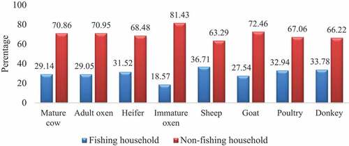
In the study area, the sampled respondents were keeping cows, oxen, heifers, calves, sheep, goats, poultry, and donkeys (Figure 3). However, non-fishing households were more possessing a large number of livestock number than fishing households. Based on research observation livestock is essential for agricultural production as traction power for the cultivation of land and income generation directly or indirectly. So, households with larger livestock holding have better access to draft power than those with less.

Figure 3. Livestock holding by sampled households (multiple responses).

Based on Table 3, related to access to fishing materials, about 25.6% and 16.8% of fishing and non-fishing households were witnessed as fishing materials are accessible in the district. On the status of access to off/non-farm activities, only 24.6% of sample households were positively responded. From sampled households, only 17.33% and 11.63% of non-fishing households and fishing households had access to credit services, respectively, from formal (Saving and cooperatives institute) and informal sources (Iqub and relatives).

Table 3. Summary of descriptive statistics for categorical variables

Variables	Values	Fishing HH (N = 172)		Non-fishing HH (N = 202)
		N	%	N	%
Access to fishing material	Yes	44	25.6	34	16.8
	No	128	74.4	168	83.2
Participation in off/non-farm activities	Yes	37	21.51	55	27.22
	No	135	78.49	147	72.78
Credit access	Yes	20	11.63	35	17.33
	No	152	88.37	167	82.67

Source: Field Survey, 2020

Sources of Income

In the study area, fishing activities were the main income source for households who participate in this sector as means of livelihood. Table 4 shows that in addition to fishing, farmers were generated income from crop production, livestock keeping/product, and off/non-farm activities. All fishing households participated in fishing and used it as the main income source while non-fishing households were participating in the cultivation of different crop types that were mainly used as the main income source. Based on the current study result fishing and crop production are the leading income source in the study area. It displays about 68.8% and 77.10% of fishing and non-fishing households were used fishing and crop production, respectively, as an income source.

Table 4. Households income sources (multiple responses)

Income source	Fishing HH (N = 172)		Non-fishing HH (N = 202)
	Frequency	Percent	Frequency	Percent
Fishing	172	68.80	-	-
Crop production	57	22.80	202	77.10
Livestock production	7	2.80	23	8.78
Livestock product	3	1.20	6	2.29
Off/non-farm activities	11	4.40	31	11.83
Total	250	100.00	262	100.00

Source: Field Survey, 2020

Of fishing households, about 22.8% of them used crop production as an additional income source. Those who are involved and used as income source through off/non-farm activities, livestock production, and the product were 4.4%, 2.8%, and 1.2% of households, respectively. For non-fishing households about 11.83%, and 11.07% of the farmers were gained additional income from off/non-farm activities and related to livestock production and products.

As information generate during focus group discussion, in addition to fishing farmers participated in producing teff, wheat, maize, and barley with a rain-based agriculture system during the rainy season (June to September). Some farmers also produce onion, tomato, and watermelon by irrigation from the end of the rainy season to the begging the next rainy season (October to May). However, the majority of sampled respondents mainly produce teff followed by wheat and maize. Those groups also stated that in the study area crop production teff has a better market price but, the majority of them were mainly cultivated for family consumption. As the survey data indicate, comparatively non-fishing households were participating in different income sources than fishing households. This is that in the study area agricultural activities other than fishing are not used by farmers as an immediate income source.

Except for fishing, other agricultural production activities took time before reaching to market; it takes several days for land preparation, sowing, growing, and harvesting in crop production for instance. Overall, in the study area, animal products like milk, egg, meat, butter, cheese, and yogurt are not mostly used in the market to generate household income due to a lack of animal feed the animal product is not enough even for home consumption.

According to Table 5, for fishing households, the main income source is fish production which generates an average income of 34,382.33 EBT which was significantly higher than other sources of income, while the annual mean income from selling animals was significantly lower than that of selling crop production, livestock product, and other non-farm activities. On other hand, all non-fishing households were generate the highest income from selling crop production which is 30,335.52 EBT. Comparatively, non-fishing households were participating in different income sources than fishing households. This is that in the study area agricultural activities other than fishing are not used by farmers as an immediate income source. Except for fishing, other agricultural production activities took time before reaching to market; it takes several days for land preparation, sowing, growing, and harvesting in crop production for instance.

Table 5. Mean annual income generated by different income sources (multiple responses)

Income source		Fishing households		Non-fishing households			T-test
	Freq.	Mean	Std. Dev.	Freq.	Mean	Std. Dev.
Fishing	172	34,382.33	6643.41	-	-	-	-
Crop	57	9051.40	5220.63	202	30,335.52	16,605.14	−9.533***
Livestock	7	3858.33	2990.72	23	8065.00	5661.53	−1.732*
Livestock product	3	4600.00	1979.90	6	11,200.00	5071.49	−1.683
Off/non-farm activities	11	5347.22	3463.73	31	6642.86	4178.60	−1.549

Source: Field Survey, 2020

4.2. Impact of Fishing on household Income in the Study Area

4.2.1. Distribution and Estimated Propensity Scores

The propensity score matching model was used to estimate propensity score matching for participant and non-participant households. As indicated earlier, the dependent variable is binary which indicates households’ participation decision in fishing activities. As Table 6 indicates, the estimated propensity scores vary between 0.0815016 and 0.9020729 with the mean value of 0.5514266 for fishing or participant households and between 0.0087808 and 0.876152 with the mean value of 0.3819536 for non-fishing or non-participant households. The common support region would then lie between 0.0815016 and 0.876152.

Table 6. Distribution of estimated propensity score

Group	Obs.	Mean	Std. Dev.	Minimum	Maximum
Total household	374	.459893	.2064071	.0087808	.9020729
Fishing household	172	.5514266	.1697708	.0815016	.9020729
Non-fishing household	202	.3819536	.203141	.0087808	.876152

Obs = Observation, Std. Dev. = Standard Deviation

Source: Field survey 2020

In other words, households whose estimated propensity scores are less than 0.0815016 and larger than 0.876152 are not considered for the matching exercise. Based on this result, fishing and non-fishing households were matched with each sample which found between 0.0815016 and 0.876152 propensity scores. Sample households outside of indicated propensity scores were not used for calculating the estimated Average Treatment Effect on Treated (ATT). This is because no matches can be made to estimate the average treatment effects on the Treated (ATT) parameter when there is no overlap between the treatment and non-treatment groups.

4.2.2. Choice of Matching Algorithm

Alternative matching estimators were used in matching the program treated and control households in the common support region. Choice of the matching algorithm was carried out from kernel bandwidth, nearest-neighbor matching, radius caliper methods. The final choice of a matching algorithm was guided by the result of mean difference, the value of pseudo-R2 and the number matched sample size. Likewise, a matching estimator which balances more independent variables has a low pseudo R² value and results in a large matched sample size was chosen as being the best estimator of the data.

Based on the result shown in the table below, kernel matching bandwidth 0.1 is the best estimator for the data that fulfilled the three main criteria in choosing a matching algorithm (Table 7). In this matching at bandwidth 0.1, all variables were insignificant in mean difference (13), relatively have low pseudo-R² (0.006), and comparatively have large matches sample size (356). So, based on these estimation results, the discussion is the direct outcomes of the kernel matching algorithm based on a bandwidth of 0.1.

Table 7. Performance of matching estimators

Matching Estimator	Performance criteria
	No. of Var. with insignificance mean the difference	Pseudo-R2	Matched sample size
Nearest Neighbor Matching
NN(1)	12	0.030	356
NN(2)	12	0.028	356
NN(3)	12	0.015	356
NN(4)	12	0.015	356
NN(5)	13	0.018	356
Caliper Matching
caliper(0.01)	13	0.018	317
caliper(0.1)	12	0.030	356
caliper(0.25)	12	0.030	356
caliper(0.5)	12	0.030	356
Kernel Matching
bwidth(0.01)	13	0.010	317
bwidth(0.1)	13	0.006	356
bwidth(0.25)	13	0.013	356
bwidth(0.5)	11	0.049	356

Source: Field Survey, 2020

According to the Table below, the pseudo-R2 and insignificant likelihood ratio vale are 0.139 and 71.54 for the unmatched sample. Additionally 0.006 and 2.82 pseudo-R2 and insignificant likelihood ration (LR chi2) vale for matched sample respectively. In the analysis result, the standardized mean difference for overall covariates used in the propensity score is 25.8% before matching. However, it was reduced to 4.0% after matching.

According to Caliendo and Kopeinind (2008) in the model output, the value of pseudo-R-square is good when its value has become low. The low value of the standard mean difference indicates that all data that were collected from both households do not have many different (distinct) characteristics. The p-values of the likelihood ratio tests indicate that the joint significance of covariates was always rejected after matching, whereas it was never rejected before matching. The pseudo- R2 also dropped significantly from 13.9% before matching to about 0.6% after matching.

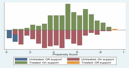
Overall, the low pseudo-R2, low mean standardized bias, high total bias reduction, and the insignificant p-values of the likelihood ratio test after matching suggest that the proposed specification of the propensity score is fairly successful in terms of balancing the distribution of covariates between the two groups. These results clearly show that the matching procedure can balance the characteristics of the treated and the matched comparison groups. All covariate balance criteria are satisfied which indicates the matching, was good. All the above tests suggest that the matching algorithm chosen is relatively best with the data that can allow estimating ATT for sampled households. Therefore, it confirms that the model is well performed to do the next model step analysis. Graph of propensity scores for treated and untreated households show a better proportion of overlap which implies a good match of propensity scores (Figure 4).

Figure 4. Distribution of propensity scores of households.

4.2.3. Average Treatment Effect on the Treated (ATT)

As Table 9 below indicates, the average treatment effect on the treated for kernel matching algorithm provides evidence as to whether or not the participant has brought significant changes to household income. The estimated average treatment effect (ATT) of sample households showed that participating in fishing has a strong and significant impact on the farm income of treated groups of smallholder farmers. The kernel matching algorithm estimator was used as the matching estimator for the data that was used to compute the average impact of fishing on rural households’ annual income. From the Table 8, it is clear that the average treatment effect on the treated (ATT) farm income of treated and untreated groups earned 36,914.85 and 31,768.43 ETB, respectively.

Table 8. Propensity score matching: quality test

Sample	Pseudo R^2	LR chi2	p> chi2	Mean bias
Unmatched	0.139	71.54	0.000	25.8
Matched	0.006	2.82	1.000	4.0

Table 9. Average Treatment Effect on the Treated (ATT)

Outcome var.	Sample	Treated	Controls	ATT	S.E.	T-stat
Annual Income	Unmatched	36,918.26	33,141.96	3776.30	1375.42	2.75**
	Matched	36,914.85	31,768.43	5146.42	1602.67	3.21**

**means significant at 5% probability levels

That is the mean farm income of the treatments is greater than the average farm income of matched (control) groups. According to the model output, the average treatment effect on the treated is about ETB 5146.42, and the mean difference in the average effect of the treatment on the treated between the matched treatment and control groups was found to be statically significant at 5% significance level. In general, participation in fishing has generated about a 7.5% increase in farm annual income of treated households over the control group. Accordingly, it is possible to conclude that participating in fishing has brought a positive impact and improved the household’s annual income status in the study area.

The results of focused group discussions and key informant interviews agree with the aforementioned results and indicated as fishing has been a good source of local people’s income than any other source of income.

The key informant interview contended as the current, national nutrition awareness has created a big demand for the fish market in the cities and small towns in the country. Especially during the fasting period of Ethiopian Orthodox religion followers; the demand raises as its highly preferred food at that time. They recognized that fishing households were mostly gained more income during fasting periods from February to April (two months), august (15 days), and November to December (45 days). Therefore, the results estimated through impact analysis of average treatment effect on treated (ATT) are in line with the situations reported by the key informant and group discussant in the study area.

This finding is consistent with Abebe and Hossein (2018) that revealed participating in fishing brought a positive and statistically significant effect on household income. Based on its conclusion, participating in fishing has contributed to change in the incomes of households in contrast to the non-fishing households implying the positive contribution of fish to diversify rural livelihood strategies and reduce rural poverty. In support of this finding, Syed et al. (2011), evaluated the impact of participating in fishing in Bangladesh and revealed that participation in this activity improved household productive income significantly.

The current finding is also in line with Heavensophy (2014), who found that the livelihood outcome of people mostly depending on fishing was better because household’s income generated from fishing was higher than income generated from agriculture, wage labor, and petty business in Tanzania coastal villages of Bagamoyo district. The result of the analysis shows that there was a statistically significant difference at a 5% level of probability between fishing and non-fishing groups on annual household income. Likewise, Yuerlita and Sylvain (2010) found that income generated from fishing was significantly higher annually than income generated from other activities in coastal people of West Sumatra Indonesia around Singkarak Lake.

4.2.4. Sensitivity Analysis

Sensitivity analysis is a recent important topic that helps to address the hidden biases or determines the magnitude of a potential unmeasured confounder (unobserved bias) which affects the conclusion. Results in Table 10, show that the inference for the effect of the participation in fishing is not changing though participant and non-participant households have been allowed to differ in their odds of being treated up to gamma = 4(100%) in terms of unobserved covariates. That means for the outcome variable estimated, at various levels of the critical value of gamma, the p-critical values are significant until gamma 4. As clearly realized from Table 10, the significance level is unaffected even if the gamma values are relaxed with an increment of 0.25. From this sensitivity analysis, we can conclude that our impact estimates (ATT) are not sensitive to unobserved selection bias.

Table 10. Result of sensitivity analysis using Rosenbaum bounding approach Rbounds delta, gamma (1(0.25)4)

Gamma()	p-critical		Hodges-Lehmann point estimate
	sig+	sig-	t-hat+	t-hat-	CI+	CI-
1	0	0	34,250	34,250	33,050	35,400
1.25	0	0	33,100	35,325	31,950	36,525
1.5	0	0	32,250	36,250	31,000	37,525
1.75	0	0	31,475	37,050	30,250	38,350
2	0	0	30,800	37,750	29,550	39,100
2.25	0	0	30,250	38,350	28,950	39,750
2.5	0	0	29,750	38,900	28,400	40,400
2.75	0	0	29,250	39,425	27,900	41,000
3	0	0	28,850	39,850	27,500	41,500
3.25	0	0	28,500	40,325	27,050	42,000
3.5	0	0	27,750	41,100	26,350	42,900
4	0	0	27,500	41,475	26,000	43,350

gamma-log odds of differential assignment due to unobserved factors

sig+ -upper bound significance level sig- -lower bound significance level

t-hat+ -upper bound Hodges-Lehmann point estimate

CI- -lower bound confidence interval (a = .95)

t-hat- -lower bound Hodges-Lehmann point estimate

CI+ -upper bound confidence interval (a = 0.95)

5. Summary and Conclusions

Agriculture remains a major livelihood of smallholder farmers in the area. The current fast population growth and increment in food demand have created an insight to see food and income diversification pathways. In the study area, the lake has been there since the 1960s and local people used to catch fish and supply it to the local markets. Fishing was considered an alternative livelihood for those who have no land and livestock for farming in the area. The sector has not gotten significant policy and research focus. The main objective of this paper is to investigate the impact of fishing on household income in lume district, Ethiopian Rift Valley. This study concluded that those who engaged in fishing have about 5146.42 Ethiopian Birr than those who were not engaged in fishing. This clearly showed as fishing has a positive and significant impact on household annual income in the study area. If the sector is supported by a conducive policy environment, it can significantly contribute toward poverty alleviation through income diversification which the country is struggling with. Regardless of the positive results, local people’s knowledge of fishing, marketing along the value chain, water hyacinth, and soil erosion due to the expansion of agricultural land in the area remain the biggest challenges for the fishing sector in the area.

In all, governmental organizations, NGOs and research institutions should focus on generating and supporting innovations that can be used to increase fish production and productivity. The local office of Agriculture and allied stokeholds should focus on how the capacity of fishermen can be further enhanced on fish catching, fish processing, and further marketing to gain more income. Special attention and extended support should be made to establishing better fishing conditions that allow the involvement of many farm households with proper lake management practices, including conserving the lake Watershed area, blocking fishing activities during the fish breeding season, allow fishing only with appropriate fishing gears and aware resource users.

Acknowledgements

We would like to acknowledge anonymous reviewers of the manuscript, data collectors, and key stakeholders engaged in the research process. We have a greater appreciation for Jimma University, College of Agriculture and Veterinary Medicine and Batu Aquatic, and other fisheries research centers for supporting this study.

Disclosure statement

No potential conflict of interest was reported by the author(s).

Additional information

Funding

The authors received no direct funding for this research.

References

- Abebe, E., & Hossein, A. (2018). Fish value chain and its impact on rural households’ income: lessons learned from Northern Ethiopia. Journal of Sustainability, 10, 37–18. https://doi.org/10.3390/su10103759
- Adamneh, D., Herzig, A., Jersabek, C. D., & Zenebe, T. (2008). Abundance, species composition and spatial distribution of planktonic rotifers and crustaceans in Lake Ziway (Rift Valley, Ethiopia). Int. Rev. Hydro Biol, 93(2).
- Alemayehu Abebe Wake and Tamiru Chalchisa Geleto. (2019). Socio-economic importance of Fish production and consumption status in Ethiopia: A review. Int J Fish Aquat Stud, 7(4), 206–211.
- Alemu, L. A., Assefa, M. J., & Tilahun, G. A. (2014). Fishery production system assessment in different water bodies of Guji and Borana zones of Oromia, Ethiopia. International Journal of Fisheries and Aquatic Studies, 2(2), 238–242.
- Ali, A., & Erenstein, O. (2017). Assessing farmer use of climate change adaptation practices and impacts on food security and poverty in Pakistan. Climate Risk Management; Elsevier, 16, 183–194.
- Amare, D., Endalew, M., Debas, T., Demissew, A., Temesgen, K., Meresa, A., & Getnet, A. (2018). Fishing Condition and Fishers Income: The case of Lake Tana, Ethiopia. International Journal of Fishery and Aquatic Science, 4(1), 006–009.
- Assefa, M. (2013). Assessment of fish products demands in some water bodies of Oromia, Ethiopia. International Journal of Agricultural Sciences, 3(8), 628–632.
- Assefa, W. W., & Abebe, W. B. (2018). GIS modeling of potentially suitable sites for aquaculture development in the Lake Tana basin, Northwest Ethiopia. Agriculture & Food Security, 7(1), 72. https://doi.org/10.1186/s40066-018-0222-0
- Ayalew, A., Fufa, A., Wubet, B., & Samson, L. (2018). Assessment of post-harvest fish losses in two selected lakes of Amhara Region, Northern Ethiopia. Heliyon, 4(11), e00949. https://doi.org/10.1016/j.heliyon.2018.e00949
- BirdLife International. (2022). Important bird areas factsheet: koka dam and lake gelila. BirdLife International. Retrieved March 28, 2022, from http://www.birdlife.org
- Brook, L. (2003). Ecological changes in two Ethiopian lakes caused by contrasting human intervention. Limnologica, 33(1), 44–53. https://doi.org/10.1016/S0075-9511(03)80006-3
- Brook, L. (2012). Report on the Value Chain Assessment of the Fishery Sector in Ethiopia. Food and Agriculture Organization Sub-Regional Office for Eastern Africa Addis Ababa, 9(4), 13.
- Caliendo, M., & Kopeinind, S. (2008). Some practical guidelines for the implementation of Propensity Score Matching. J.Econ.Surv, 22(1), 31–72. https://doi.org/10.1111/j.1467-6419.2007.00527.x
- Dawit, G., Asefa, A., Gezahegn, A., & Fekadu, B. (2013). Analysis of the significance of fishing on the food security status of rural households around Lakes Ziway and Langano in Ethiopia. J. Econ. Sust. Develop, 4(18), 1–10.
- De Graaf, G. J., & Garibaldi, L. (2019). The Value of African Fisheries. FAO. Pp67.
- Endalew, B., Zeleke, M., Yenewa, W., Ayalew, Z., & González-Redondo, P. (2020). Determinants of farm households’ participation in fish production in Southwest Ethiopia. Cogent Food & Agriculture, 6(1), 1728107. https://doi.org/10.1080/23311932.2020.1728107
- Ethiopian Ministry of Agriculture (MoA), (2020): Challenges for Ethiopia’s agriculture sector policy and investment framework: (Draft Final Report), Addis Ababa.
- FAO. (2020). The State of World Fisheries and Aquaculture 2020. Food and agriculture organization of the United Nations.
- Food and Agriculture Organization (FAO). (2018). The state of world fisheries and aquaculture, meeting the sustainable development goals, food and agriculture organization of the United Nations.
- Gatriay Tut Deng. (2020). Assessment of factors affecting fish production and marketing in gambella region, Ethiopia. The Scientific World Journal.
- Gebrehiwot, T., & Anne Van Der, V. (2015). Estimating the impact of food security program by propensity score matching. Journal of Development and Agricultural Economics, 7(1), 38–47. https://doi.org/10.5897/JDAE2014.0585
- Golubtsov, A. S., & Redeat, H. (2010). Fish faunas of the Chamo-Abaya and Chew Bahir basins in the southern portion of the Ethiopian Rift Valley origin and prospects for survival. Aquat. Ecosyst. Health Manage, 13(1), 47–55. https://doi.org/10.1080/14634980903578506
- Heavensophy, M. (2014). analysis of economic determinants for households involvement in fishing for livelihoods, a dissertation submitted in partial fulfillment of the requirements for the degree of master of science in environmental and. Natural Resource Economics of Sokoine University of Agriculture.
- Husien, S., Mahmud, K. T., Islam, M. T., & Shihab, M. A. (2016). Small credit for big opportunities: A case of BRAC’s agribusiness program in Bangladesh. International Journal of Economics and Finance, 8(1), 7–14. https://doi.org/10.5539/ijef.v8n1p7
- Kothari, C. R. (2004). Research Methodology: Methods and Techniques. New Age International Publishers.
- Lemma, A., Abebe, G., & Brook, L. (2014). Composition of commercially important fish species and some perspectives into the biology of the African Catfish Clarias gariepinus (Burchell), Lake Ziway, Ethiopia. International Journal of Advanced Research, 2(1), 864–887.
- Lume District office of Agriculture (2020): Performance of Fisheries and Agricultural sector in the district; Office Report, Modjo.
- Ministry of Agriculture (MoA) (2020): Challenges for Ethiopia’s agriculture sector policy and investment framework: (Draft Final Report), Addis Ababa.
- Olale, E., & Henson, S. (2013). The impact of income diversification among fishing communities in Western Kenya. Food Policy Report, 43, 90–99. https://doi.org/10.1016/j.foodpol.2013.08.008
- Olaoye, O., Ashley-Dejo, S., Fakoya, E., Ikeweinwe, N., Alegbeleye, W., Ashaolu, F., & Adelaja, O. (2013). Assessment of socio-economic analysis of fish farming in Oyo State, Nigeria. Global Journal of Science Frontier Research Agriculture and Veterinary, 13(9), 45–55.
- Riehl, B., Zerriffi, H., Naidoo, R., & Bauch, C. T. (2015). Effects of Community-Based Natural Resource Management on Household Welfare in Namibia. PLoS ONE, 10(5), 1–23. https://doi.org/10.1371/journal.pone.0125531
- Rosenbaum, P. R., & Rubin, D. B. (1983). The central role of the propensity score in observational studies for causal effects. Biometrika, 70(1), 41–55. https://doi.org/10.1093/biomet/70.1.41
- Syed, M., Aminur, R., Ariful, H., Syed, M., & Ashrafur, R. (2011). Impact of fish farming on household income: a case study from mymensingh district. Journal of Social Sciences, 7(2), 127–131. https://doi.org/10.3844/jssp.2011.127.131
- Tesfaye, G., & Wolff, M. (2014). The state of inland fisheries in Ethiopia: A synopsis with updated estimates of potential yield. Ecohydrology and Hydrobiology, 14(3), 200–219. https://doi.org/10.1016/j.ecohyd.2014.05.001
- Tilahun, A., Alambo, A., & Getachew, A. (2018). Fish production constraints in Ethiopia: A review. World Journal of Fish and Marine Sciences.
- Vijverberg, J., Dejen, E., Getahun, A., & Nagelkerke, L. (2012). The composition of fish communities of nine Ethiopian lakes along a north-south gradient: Threats and possible solutions. Animal Biology;, 62(3), 315–335.
- World Bank (WB). (2012). The global contribution of capture fisheries. Economic and Sector Work Report, (66469).
- Yuerlita, K., & Sylvain, R. (2010). Livelihood features of small scale fishing communities: A case from Singkarak Lake, West-Sumatra, Indonesia. International Journal of Environment and Rural Development, 1(2), 94–101.
- Zinabu, G. M. (2002). The Ethiopian Rift Valley lakes major threats and strategies for conservation. Ethiopian Rift Valley Lakes. Backhuys.