The effect of foreign direct investment on structural transformation in developing countries

Abstract

This paper investigates the effects of foreign direct investment (FDI) on structural transformation using panel data from 44 developing countries and four newly industrialized countries from 1990 to 2018 by employing the generalized method of moment approach of Arellano-Bond (1991). The estimated results suggest that FDI inflows have a positive significant effect on the structural transformation. In addition, the paper explores the channels through which FDI affects structural transformation. The Principal Component Analysis (PCA) indicates that structural change contributes 55.95 percent to structural transformation, followed by capital accumulation (37.92 percent) and economic growth (6.13 percent). Particularly, manufacturing and service-sector output and employment growth, as well as urbanization, are major pathways via which FDI fosters structural transformation in developing countries. Therefore, special consideration should be given to FDI motivated by manufacturing exports, as well as policies that boost absorption capacity and enable labor mobility in developing countries.

Keywords:

• foreign direct investment
• structural transformation
• structural change
• economic growth
• developing countries

PUBLIC INTEREST STATEMENT

Structural transformation is crucial, but it is still difficult to achieve in developing countries due to low domestic resources, a lack of technology and managerial expertise, and a low development of the industrial sector to lead it. FDI plays a major role in structural transformation by making capital investments in the industry sector, transferring cutting-edge technology and managerial skills, and linking the local economy with the global market. Our empirical research also implies that it fosters structural transformation by allowing for increased manufacturing-sector production and employment as well as boosting urbanization, capital accumulation, and economic growth in developing countries. In order to benefit the most from FDI, countries should work to attract a significant quantity of it, especially in the manufacturing sector, by offering various incentives and enhancing domestic absorption capability.

1. Introduction

Structural transformation is the lifeblood that allows development to be accomplished in developing countries (Chenaf-Nicet, 2019; Khan, 2020). Countries that have undergone structural transformation have been able to escape poverty and become prosperous (Marjanovic, 2015). It is a complex concept that, besides economic growth and capital accumulation, also compresses structural changes in economic structure, social area, and technology (Chenery, 1960: Chenery et al., 1986). Becoming structurally transformed will be achieved through three different stages. In the early stages of the structural transformation, the share of agriculture of labor force is large with very low productivity but start to decline (Rodrik, 2018). A country in the early stage of structural transformation is typically composed of 20, 30 and 50 percent of Gross Domestic Product (GDP) from industry, services and agriculture, respectively, while its share of workers comes in at 9.7, 20.8 and 69.5 percent from each of these sectors (Timmer & Akkus, 2008). At this stage, industry is established to satisfy the essential demands of the society such as food, textiles and clothing (Syrquin & Chenery, 1989). The second stage is marked by a change in the economy’s center of gravity away from primary output and toward manufacturing (Chenery et al., 1986). At the final stage of structural transformation, the economy will be dominated by the service sector, with an important but diminishing industry sector (Faruqi & O’Brien, 1976). At this stage, employment in the agriculture-sector accounts for less than 5 percent of total employment and the economy is said to be developed (Syrquin & Chenery, 1989). In general, structural transformation is marked by a constant decrease in the share of labor dedicated to agriculture through time, a steady increase in the share of labor allocated to services, and a hump-shaped pattern in the share of labor allocated to manufacturing (Duarte & Restuccia, 2010).

In the 1960s, Asian Tigers (Singapore, South Korea, Taiwan, and Hong Kong) had economic levels comparable to that of today’s developing nations, for example, Ethiopia, but they succeeded in structural transformation and became developed (Awaliyyah et al., 2020). Other major Asian countries, such as China and Thailand, are on track with structural transformation, but Africa and Latin America developing countries are still facing significant challenges (Bah, 2011; McMillan et al., 2014). For instance, smallholder farms constitute more than 80 percent of all farms in Sub-Saharan Africa (SSA), and agriculture employs a disproportionately large proportion of the population across most African countries (example—92, 89, 75, & 68 percent in Burkina Faso, Burundi, Ethiopia & Kenya, respectively), and accounting for more than 40 percent of the GDP in some countries, including Mali, Ethiopia, Niger, Central Africa Republic, and Chad, which are important indicators of Africa’s poor structural transformation (McMillan & Headey, 2014). These indicates that structural transformations in developing countries are not running optimally, and even lag behind due to a variety of challenges.

The first challenge is ensuring a sustainable economic growth, which is a prerequisite for structural transformation and crucial for poverty alleviation, but, in a context where widespread poverty is prevalent, there will be little saving and investment, leading to low growth (Mensah et al., 2016). Low productivity is another challenge of structural transformation of developing countries. As per this idea, domestic savings should be mobilized to increase productivity via capital accumulation, but developing countries have failed to do so because they still have three gaps: the saving-investment gap, the revenue-expenditure gap, and the export-import gap (Anyanwu, 2017; McMillan et al., 2014). Manufacturing is still in its infancy, as it does not have a sufficient capital base to absorb a huge labor force and it is not capable of leading structural change in developing countries (Hauge, 2019). Some existing industries are also incompetent and abandon the market, displacing workers and forcing them to migrate from manufacturing to agriculture and the informal sector particularly in Latin America and Africa (Bah, 2011; McMillan et al., 2014). Moreover, due to limited industrial sectors, developing countries are transitioning directly from agriculture to service economies without having had a complete experience of industrialization—this transition is called premature deindustrialization (Rodrik, 2018).

Therefore, Foreign Direct Investment (FDI) is one of the most effective tools for achieving structural transformation in developing countries, as it allows them to break the cycle of poverty and address resource scarcity (Hauge, 2019). In the short term, FDI can assist host countries in accumulating physical capital by increasing income through large-scale job creation, increasing foreign currency and tax revenue, expanding the global market opportunities, and finally influencing infrastructure and the business environment, all of which are required inputs for structural transformation (Mamba et al., 2020). FDI contributes, usually in the long run, to structural transformation of the host economy through the development of productive capabilities and industrialization through technology transfer and managerial skills, market and technology linkages to the host country, shifting labor and other resources from low- to high-productivity sectors, competitive pressure on domestic companies, and human capital development (Gui-Diby & Renard, 2015).

Although economic growth is one part of structural transformation, empirical studies have focused on it, and little research has been done on the effect of FDI on structural transformation. For instance, studies conducted by Gui-Diby and Renard (2015), Samouel and Aram (2016), Mensah et al. (2016), Jie and Shamshedin (2019), Mamba et al. (2020), Oduola et al. (2022), and Muller (2021) are limited to Africa; others such as Muhlen and Escobar (2020), Thirion (2020), Montes and Cruz (2020), and Maroof et al. (2019) are corresponding to Asia; and studies of Topcu (2016), and Chenaf-Nicet (2019) addressed the issue in developing countries, but they focused on higher middle-income countries. These little studies also used structural change (the share of industry/manufacturing employment or output) as a measure of structural transformation. It can be misleading to use structural change alone as a measure of structural transformation, since structural change is a necessary but not sufficient condition for structural transformation. Thus, this study aims to address these gaps by examining the role of FDI in structural transformation focusing on countries from all or most regions by their level of structural transformation with the aim of drawing lessons for developing countries.

The rest of the paper is structured as follows: The review of pertinent theoretical and empirical studies is presented in section 2, and the study’s methodology (study area, data sources, model specification, and estimation techniques) is presented in section 3. Section 4 presents the results and discussion. The concluding remarks of the paper, with policy implications, appear in section 5.

2. Literature review

Among early structural transformation theories, Lewis theory claims that structural transformation consists of the re-allocation of surplus agricultural labor to industry (Syrquin, 2010). This is just a two sector model that attempts to explain only labor movement. Alternatively, Rostow (1959) conceptualized structural transformation as a change in the rate of accumulation of capital (Rostow, 1956 &, 1959) but it also limited the conceptualization of structural transformation mainly to the accumulation of physical capital. Ranis and Fei (1961) heavinly based on Lewis theory, the only difference with Lewi theory is the turing up point of zero marginal produductivity labor supply from the agriculture. Kuznets (1973) also suggests that as a country develops, there is increase in non-agricultural sector output share, rural to urban migration, and the share of manufacturing goods. This theory has also been chastised for being based on the circumstances of industrialized countries, which may not reflect the true picture of developing countries. The most relevant theory of structural transformation was presented by subsequent works of Chenery. Chenery (1960) and H. Chenery and Syrquin (1975) pointed out that structural transformation is mainly characterized by (i) per capita income increase, (ii) accumulation of capital, (iii) structural change in production, demand, demography, income distribution, and international trade. It is critical to use it as a foundation for this empirical research analysis, despite the fact that it was conceptualized in the mid to late 1970s and has little relevance to current events, and uses each dimension separately to show structural change and transformation rather than making a composite index.

A review of empirical studies is essential to fill this gap. Empirically, for instance, Gui-Diby and Renard (2015) in 49 African countries, Mensah et al. (2016) in 21 countries, Topcu (2016)’s study on 19 upper middle-income developing countries, and Mamba et al. (2020) in West African Economic and Monetary Union (WAEMU) suggest that FDI has not a significant effect on structural transformation. On the other side, Samouel and Aram (2016) from Africa, Jie and Shamshedin (2019)’s Vector Error Correction Model (VECM) estimation in Ethiopia, and the findings of fixed effect estimation’s of Muhlen and Escobar (2020) and Thirion (2020) from Mexico show that FDI is significantly beneficial to industrialization. They noted that a significant contribution of FDI is connected to Greenfield FDI’s ability to reallocate labor effectively from the primary sector to the industrial sector, as well as its ability to create jobs.

Contrarily, Maroof et al. (2019)’s estimate of the Autoregressive Distributed Lag (ARDL) of South Asian economies for 1996–2015, Oduola et al. (2022) GMM’s estimate in 43 SSA countries from 1996 to 2018, and Muller (2021) PCSE’s output in 47 SSA countries from 1996 to 2017 suggest that FDI has a significant negative effect on industrial development due to repatriation of profit and market setting effects, as well as the deterioration of domestic welfare. They also noted that primary sector FDI, especially oil exploration and mining FDI, and inadequate institutional characteristics were identified as rationales for FDI obstacles to structural transformation in the selected nations.

To summarize, all empirical studies used a single aspect of structural transformation to measure it, such as the share of manufacturing GDP or employment, which is not a comprehensive approach to measuring structural transformation. Another gap is that no scientific research on FDI’s contribution to structural transformation has been conducted in developing countries involving countries from different continents (Africa, Asia, and Latin America). As a result, we attempted to add to the literature by developing a structural transformation index and using countries from various continents as a sample unit.

3. Methodology

3.1. Selected countries

First, this study attempted to distinguish between developing and developed countries. The World Bank’s per capita income-based criteria are widely used to designate countries as developed or developing. However, it has been criticized for focusing on only one factor of development and failing to consider other important dimensions of development such as education, health, and others (Kinnunen et al., 2019). Hence, we selected developing countries based on the United Nations’ Human Development Index (HDI) criteria, which considers numerous elements, including a long and healthy life, knowledge, and a reasonable living standard. Then, we tested whether there is any data available on the theoretical factors that contribute to structural transformation in developing countries. The known source for structural transformation data, the Groningen Growth and Development Centre (GGDC) website, provides structural transformation data only for 44 developing nations, as shown in Table 5 under section 4.1 for the period 1990–2018. Finally, to understand how FDI explains the difference in transformation performance, we must compare countries that failed to transform their economy (or are in the midst of transitioning) to those that are industrialized. Thus, we included Asian Tigers/Newly Industrialized Countries (NICs)—notably Taiwan, Singapore, Hong Kong, and South Korea—in the study to compare because they were in a similar situation 5–6 decades ago as developing countries are today (Awaliyyah et al., 2020).

3.2. Data and model specification

The following Equation (1) is shows the model specification FDI-Structural transformation:

(1) $lnST{I}_{it}={\beta }_0+{\beta }_{1}lnST{I}_{i,t-1}+{\beta }_{2}lnFD{I}_{it}+{\beta }_{3}lnA{L}_{it}+{\beta }_{4}lnO{T}_{it}+{\beta }_{5}lnPo{p}_{it}+{\epsilon }_{it}$(1)

For i = countries {1, … 44} and t = time period measured by years (1990, …, 2018), STI = structural transformation index, β₀ is the value structural transformation when there are no factors, β₁—β₅ measures the effect of respective variable on STI, and ε = error term. STI is for structural transformation index, FDI stands for foreign direct investment, OT stands for openness of trade, AL stands for arable land, and PoP stands for population. The definitions, measurements, and expected signs of the variables used in the FDI-structural transformation analysis are shown in Table 1.

Table 1. Definition, measurement, and expected signs of variables

Symbol	Definition & Hypothesis	Data Source
STI	It is a dependent variable in FDI-Structural transformation regression analysis. The STI is a composite index that includes the following components: (1) per capita GDP, (2) physical capital accumulation, (3) human capital, (4) service sector employment, (5) manufacturing employment, (6) urban population, (7) agriculture value-added output, and (8) manufacturing export. Because just one lag of STI (STIt-1) is included in the model, there is no need to incorporate one or more variables that were involved in STI creation as explanatory variables in the FDI-STI regression analysis. The addition of variables results in a duplication of variables. Hence, we included total population, arable land, and trade openness as control factors in our FDI-STI regression study, in addition to our interesting variable FDI.	-
lnFDI	It is the amount of equity capital, earnings reinvestment, and other intra-firm loans represented as net FDI inflows in the balance of payments. It is measured in terms of stock by USD at current prices in millions. It is projected to have a favorable effect on structural transformation because it is a source of cash, technology, and knowledge. Therefore, the study tried to test against the null hypothesis that states FDI has no effect on structural transformation in developing countries.	UNCTAD
lnOT	A country’s trade openness can be defined using the ratio of exports plus imports over GDP. It is calculated as a percentage of GDP. Liberalizing trade increases foreign direct investment, job opportunities, and economic integration with the world market, resulting in increased income for unskilled labor, capital accumulation, and technology transfers, all of which are crucial for structural transformation in developing countries. (McMillan et al., 2014). It’s also regarded as a barometer of an institution’s quality (Uy et al., 2013). Hence, it is anticipated that it will have a beneficial effect on structural transformation.	UNCTAD
lnAL	It is defined as the land under temporary agricultural crops, meadows for mowing or pasture, land under market and kitchen gardens and land temporarily fallow. It is measured by hectare (thousand). Agriculture-based-MNEs need natural resource endowments, which are proxied here by the logarithm of the area of arable land, to invest directly in agribusiness like crop production and indirectly in supply chain linkage (Suleman, 2009). Agriculture is also a significant source of domestic capital, employment, and GDP growth in developing nations; so, transformation cannot be completed without considering agriculture, particularly the potential for arable land. Hence, it is predicted to have a favorable effect on structural transformation.	FAO
lnPoP	The population is an important device for attracting FDI since it provides both cheap labor and a vast market.	UNCTAD

UNCTAD = United Nations Conference on Trade and Development; FAO = Food and Agriculture Organization

Our dependent variable, structural transformation, is a composite index of eight variables, as shown in Tables 1 and 2. Therefore, Principal Component Analysis (PCA) was applied to develop a structural transformation index. It is superior to conventional mechanisms for creating structural transformation indexes because it avoids double counting, removes correlated features, improves algorithm speed, decreases overfitting, and enhances visualization (Granato et al., 2018; Gygli et al., 2019; JRCEC, 2005; Watkins, 2018). The selection of theoretically relevant variables for index development is the first step in PCA (Alavin et al., 2020). Variables like (1) per capita GDP (PcGDP), (2) per capita physical capital (PcCA), (3) human capital (HC), (4) urban population share (UP), (5) service-sector employment share (SE), (6) manufacturing employment share (ME), (7) agriculture value-added output share (AVA), and (8) manufacturing export share (MEXP) are chosen for structural transformation index based on theoretical considerations, data availability, and statistical tests. For example, institutional, dietary, and attitude changes in societies are markers of structural transformation, but due to a lack of data, they are unable to be included; similarly, manufacturing and service-sector outputs have both fallen dramatically due to the multicollinearity problem. Table 2 shows the definitions, measurements, and predicted indications for the eight variables given above.

Table 2. Definition, measurement, data source, and expected signs of structural transformation variables

Symbol	Definitions of Variables and Expected Signs	Data Source
PcGDP	Kuznets (1966) linked structural transformation to long-term economic growth, which he described as a country’s ability to deliver increasingly diverse economic goods to its population. Since this study uses per capita GDP as a proxy for sustainable economic growth, its effect on structural transformation is predicted to be favorable.	UNCTAD
HC	Human capital is defined as an individual’s stock of knowledge, skills, and other attributes that enable them to be more productive. The endogenous growth theory of Romer (1990) suggests that an economy with a large stock of human capital will grow faster and undergo structural transformation easily. Thus, it is thought to have a good influence on structural transformation	PenT10.0
PcCA	It is measured by per capita capital accumulation, which is the ratio of gross fixed capital formation at current prices in millions over the entire population. In Harrod (1939)-Domar (1947) growth theory and Rostow (1956) linear stage theory, capital accumulation is suggested to be an important indicator of structural transformation and sustainable growth. Hence, it is predicted to have a favorable impact on structural restructuring.	UNCTAD
UP	Kuznets (1966) defines structural transformation as a shift in population distribution between rural and urban areas, with the share of urban population increasing as the country becomes structurally transformed.	UNCTAD
MEXP	According to Chenery’s (1960) structural change hypothesis, having a higher share of manufacturing export in merchandise export is a good indicator of structural transformation. Manufacturing exports are calculated as a percentage of overall merchandise exports in this case. As a result, it is predicted to have a favorable impact on structural transformation.	WTO
ME	It is the proportion of manufacturing employment in total employment. Under Lewis’s (1954) model of dualistic development, structural change is defined as a gradual transition of employment from agricultural to manufacturing sector. Hence, a large proportion of it is a favorable signal of structural transformation and is likely to have a positive effect on it.	GGDC
SE	According to structural theory developed by H.B. Chenery and Taylor (1968) and Syrquin and Chenery (1989), a continued increase in service employment is one indicator of structural transition. It is expressed as a proportion of total employment held by the service industry. It is anticipated that it will have a positive impact on structural transformation.	GGDC
AVA	According to Syrquin and Chenery (1989) theory, structural transformation is manifested by the continual decline in agriculture’s value-added share of total output. A percentage proportion of agriculture value-added output in total output is used to calculate it. It is anticipated that it will have a positive effect on structural transformation.	GGDC

UNCTAD = United Nations Conference on Trade and Development, WTO = World Trade Organization, PenT10.0 = Pen Table 10.0, FAO = Food and Agriculture Organization, GGDC = Groningen Growth and Development Centre.

Because the selected variables were measured by different units, normalizing them to a uniform scale ranging 0 to 1, with 1 as the highest value and 0 as the lowest value, is the second step in PCA (Iezzoni & Pritts, 1991). Max-Min rescaling is the best method to use for data re-scaling because it has fewer misclassification errors than other methods, and it maintains relationships between original data values more efficiently than other methods (Aksu et al., 2019; Hajkowicz, 2006; Saranya & Manikandan, 2013). Third, the selected variables should be checked to make sure they are adequate before the PCA analysis is carried out. It is common to use Kaiser–Meyer–Olkin (KMO) to assess sample adequacy (MSA) and the appropriateness of data for PCA (Olawale & Garwe, 2010; Shrestha, 2021). Depending on the value of KMO, it is unacceptable if it is less than 0.5, mediocre if it ranges between 0.50 and 0.70, good if it ranges between 0.70 and 0.80, excellent if it ranges between 0.80 and 0.90, and remarkable if it is above 0.90 (Mohamad et al., 2017). Hence, our sample is good enough to perform PCA analysis based on KMO’s calculated value of 0.8119. The fourth stage in PCA is to run it and identify how many components (group of variables) there are. Bauman and Chenoweth (1984) suggest three general criteria to determine the number of components: (i) factors with eigenvalues closer to or greater than 1, (ii) factors with individual contributions to variance exceeding 10 percent, (iii) factors with cumulative contributions to variance exceeding 70 percent. The eigenvalue is a measure of how much of the variance of the observed variables a factor explains. In Table 3, according to Bauman and Chenoweth (1984), the first three components are selected and the rest are rejected.

Table 3. Engenvalues of structural transformation

Component	Eigenvalue	% of variance explained	Cumulative %
Comp1	4.43218	0.5540	0.5540
Comp2	1.09951	0.1374	0.6915
Comp3	0.940133	0.1175	0.8090
Comp4	0.569173	0.0711	0.8801
Comp5	0.348905	0.0436	0.9237
Comp6	0.272825	0.0341	0.9578
Comp7	0.213103	0.0266	0.9845
Comp8	0.12417	0.0155	1.0000

Common factor 1 has an eigenvalue of 4.4322 and individual and cumulative contributions of 55.40 percent, which implies that this common factor explains about 55.40 percent of the overall variance of the eight structural transformation indicators. Common factor 2 has eigenvalue of 1.099, and individual contribution of 13.74 percent and a cumulative contribution of 69.15 percent. Common factor 3 has an eigenvalue of 0.9401 which is very close to 1 and an individual contribution of 11.75 percent. Overall, these three common factors cumulatively explain 80.90 percent of the overall variance. Factors 4, 5, 6, 7 and 8 are not used for constructing composite index because they fail to meet three criteria outlined above.

Make rotation is the fifth stage in PCA. A key objective of rotation is to make each variable’s contribution as simple, understandable, and replicable as possible (Olawale & Garwe, 2010). There have been two rotation methods, Orthogonal is used when the components are orthogonal to each other and Oblique when they are not (Abdi & Williams, 2010; Yong & Pearce, 2013). Therefore, we used Oblique-Promax rotation since we assumed that the variables in the study would be correlated. A factor loading of greater than 0.4 is generally considered to be an eligible variable for inclusion in index construction (Alavin et al., 2020); therefore, as shown in Table 4, all included variables grouped under three common factors are eligible.

Table 4. Common factors and weight analysis

Variables	Common factor loading			Squared Factors loading (Scaled to sum to one)			Weight
	Comp1	Comp2	Comp3	Comp1	Comp2	Comp3
HC	0.4193	0.0409	0.1636	0.1757	0.0017	0.0267	0.0687
PcCA	−0.0102	0.0162	0.9664	0.0001	0.0003	0.9335	0.3112
PcGDP	0.418	−0.0677	0.0688	0.1746	0.0046	0.0047	0.0611
SE	0.4656	−0.0125	0.0258	0.2166	0.0001	0.0006	0.0725
MEXP	−0.0672	0.7368	0.0691	0.0045	0.5423	0.0048	0.1825
UP	0.5085	−0.0946	−0.1053	0.2584	0.0089	0.0111	0.0916
AVA	−0.41	−0.1387	0.1167	0.1679	0.0192	0.0136	0.0679
ME	0.0461	0.6506	−0.0697	0.0021	0.4228	0.0048	0.1433

As shown in Table 4, common factor 1 contains five variables: HC—human capital (0.4193), PcGDP—per capita income (0.418), SE—services sector employment share (0.4656), UP—the share of urban population (0.5085), and AVA—agriculture value-added output share (−0.41). The negative sign of agricultural value-added share indicates that a decrease of it increases the structural transformation. Common factor 2 contains only two variables with factor loadings exceeding 0.400—manufacturing export share (0.7368) and ME—manufacturing employment share (0.6506), Common factor 3 contains only one variable called PcCA—per capita capital accumulation (0.9664), but all other variables are already allocated to components 1 and 2 with higher factor loading.

Finally, to assess each variable’s proportionate contribution to a common component, we squared the factor loadings and scaled them to unity to make comparisons across variables easier. The following formula (Equation 2) is used to calculate the relative contribution of each of the eight variables to the structural transformation index, which is shown in the last column of Table 4:

(2) $W_j={\sum }_{ij}{h}_{ij}^2/({\sum }_{ij}{h}_{i1}^2+{\sum }_{ij}{h}_{i2}^2+{\sum }_{ij}{h}_{i3}^2+{\sum }_{ij}{h}_{i4}^2+{\sum }_{ij}{h}_{i5}^2+{\sum }_{ij}{h}_{i6}^2+{\sum }_{ij}{h}_{i7}^2+{\sum }_{ij}{h}_{i8}^2$(2)

where: W is estimated weight, h² represents communality that is the variance that due to a single variable, i is the component dimension (i = 1, 2, 3), and j is the variable dimension (j = 1 represents human capital, 2 is capita capital stock accumulation, 3 is per capita income, 4 service-sector employment share, 5 is the share manufacturing export in total merchandise export, 6 is the share of urban population, 7 is the share of agricultural value-added output, and 8 is the share of manufacturing sector employment in total employment).

Table 5. Structural transformation status of the countries

No	Country	STI	No		STI	No	Country	STI
1.	Taiwan	0.8363	17.	Brazil	0.5325	33.	Ghana	0.3278
2.	Hong Kong	0.8296	18.	Argentina	0.5305	34.	Senegal	0.317
3.	South Korea	0.8079	19.	South Africa	0.4951	35.	Nepal	0.3146
4.	Singapore	0.8012	20.	Bangladesh	0.481	36.	Kenya	0.286
5.	Malaysia	0.7983	21.	Pakistan	0.4786	37.	Zambia	0.2531
6.	Mexico	0.6993	22.	Morocco	0.4643	38.	Cameroon	0.2526
7.	Cambodia	0.6932	23.	Colombia	0.4633	39.	Myanmar	0.2521
8.	Mauritius	0.6802	24.	Bolivia	0.4586	40.	Tanzania	0.228
9.	Turkey	0.6363	25.	Lesotho	0.4431	41.	LAO	0.2088
10.	China	0.6304	26.	India	0.4386	42.	Uganda	0.1978
11.	Thailand	0.5911	27.	Viet Nam	0.4367	43.	Nigeria	0.1915
12.	Tunisia	0.5906	28.	Indonesia	0.4324	44.	Rwanda	0.143
13.	Sri Lanka	0.5752	29.	Peru	0.4137	45.	Burkina Faso	0.136
14.	Philippines	0.5607	30.	Ecuador	0.4006	46.	Mozambique	0.136
15.	Botswana	0.5561	31.	Egypt	0.395	47.	Malawi	0.1294
16.	Costa Rica	0.5543	32.	Namibia	0.3726	48.	Ethiopia	0.0951

No = Role number.

Based on the characteristics of variables, we grouped the eight variables into three broad categories; (i) structural change (includes service-sector employment, manufacturing export, urban population, agricultural value-added output, and manufacturing employment), (ii) capital accumulation (per capita physical accumulation and human capital), and (iii) per capita income. As shown in the last column of Table 3, structural change accounts for 55.95 percent of the overall weight, followed by capital accumulation (37.92 percent) and per capita income (6.13 percent) in the index of structural transformation. The Structural Transformation Index (STI) is then computed as

(3) $\mathrm{S}\mathrm{T}{\mathrm{I}}_{\mathrm{i}\mathrm{t}}=\sum W_{cit}\ast X_{cit}$(3)

where the letter c stands for indicator dimension (c = 1,—, 8), i stands for country dimension (i = 1, 1, … ., 48), t stands for time dimension (t = 1990,—-, 2018). $W_{cit}$ is estimated weight, X_cit indicates the variables that comprise the structural transformation index, STI_it is composite structural transformation.

As one of three components of structural transformation (structural change, capital accumulation, and economic growth), structural change is the most important. In addition to focusing on FDI’s effect on structural transformation, this study also sought to understand how FDI effects structural change in developing countries. To do so, the study tried to investigate the effect of FDI on: (i) manufacturing output, (ii) service-sector output, (iii) manufacturing-sector employment, (iv) service-sector employment, (v) manufacturing export, and (vi) urbanization. For this purpose, the model specification is presented in Equation (4):

(4) $ln{Y}_{it}={\beta }_0+{\beta }_{1}lnFD{I}_{it}+{\sum }^{l}n{X}_{it}+{\epsilon }_{it}$(4)

where: Y_it is a dependent variable; in our case, structural change indicators such as the share of manufacturing employment (in logarithm form), the share of manufacturing value-added output (in logarithm form), the share of manufacturing export in total merchandise export, the share of services-sector employment (in logarithm form), the share of service-sector output (in logarithm form), and urbanization measured by the share of urban population in total population. X_it refers to a set of control variables (PcGDP, physical capital accumulation as a percentage of GDP, human capital, arable land, openness of trade, and total population). To lessen the difficulties with outliers, all control variables are employed in their logarithmic form.

3.3. Estimation methods

There are three panel data estimation approaches that are widely used: (i) Pooled OLS (POLS), (ii) Fixed Effect (FE) estimation, and (iii) Random Effect (RE) estimation. POLS estimates panel data using the OLS method, which assumes a constant slope and intercept and ignores time and individual dimensions (Cornwell & Rupert, 1988; Gujarati, 2003). FE provides for heterogeneity or individuality among various cross-sections, enabling each cross-section to have its own intercept while being constant across time (Gujarati, 2003). Although RE allows for heterogeneity and is time invariant, the individual’s specific effect is unrelated to the independent variable (Greene, 2003). The Hausman specification test is used to determine if the RE is a suitable model to test against the FE. If the p-value of the test is greater than 0.05, we do not reject the null hypothesis and it implies that RE is consistent and efficient. If this is the case, then we further test POLS against RE by using Beush-Pagan’s Lagrange Multiplier (LM) test; if the null hypothesis is not rejected, the POLS is better otherwise RE. Alternatively, we reject the null hypothesis if the Hausman test shows a p-value less than 0.05. This suggests that FE is better than RE. Then, we used the F-test to compare POLS to FE; if the null hypothesis is rejected in the F-test, the FE is preferable. Using the Hausman Test and F-test outputs, as shown in Table 9, we estimated the model specified in Equation (4) with the FE estimation method.

However, it is problematic for FE to be used in the context of a dynamic model (a model with a lagged dependent variable as a right hand side variable) like model as shown in Equation (1) because it is not able to account for the endogenous component of the lagged dependent variable. It makes the panel estimation of the conventional FE and RE inconsistent (Teixeira & Queiros, 2016). For the dynamic model, the most popular option is Arellano-Bond (1991) generalized method of moment (GMM) estimation, which deals with the endogeneity problem through internal instruments by differencing the included variables (Moral-Benito et al., 2018; Samouel & Aram, 2016). Additionally, it allows for some degree of endogeneity in the other explanatory variables (Fukase, 2010). The method’s fundamental tenet is to start with the first difference in the regression equation and work backwards to eliminate the individual-fixed effects. The lagged variable will thus be viewed as the difference equation’s corresponding instrumental variable for the endogenous variables. Therefore, Arellano-Bond (1991) GMM is used in this study. This study used STATA 16.0 to process data for the descriptive analysis and regression.

4. Results and discussions

There are two subsections in this section. The descriptive analysis of the structural transformation status and its indicators is presented in the first section. The econometric analysis of FDI-structural transformation and the effect of FDI on structural change are thoroughly presented in the second section.

4.1. Descriptive analysis

Table 5 presents the average structural transformation status, from 1990 to 2018, for 44 developing countries and 4 newly industrialized countries. The closer the structural transformation is to 1, the more successful the structural transformation is, but if the value near 0, the structural transformation is bad. NICs have STI values greater than 0.8, so we may use 0.8 as a threshold to judge a country structurally transformed if STI is equal to or greater than 0.8, unless the country is structurally transforming (non-transformed).

Asian nations such as Malaysia, Cambodia, Turkey, China, Thailand, Sri Lanka, and the Philippines occupy the position next to NICs in Table 5. Latin American countries such as Mexico, Brazil, and Argentina were next in line. Mauritius, Tunisia, Botswana, and South Africa are among the African countries that have competed with Asian and Latin American countries. Table 5 demonstrates that Ethiopia, often known as the African lion/tiger, and other African nations such as Malawi, Mozambique, Burkina Faso, Rwanda, Nigeria, and Uganda have seen very little structural transformation and are still in the early stages of industrialization.

As seen in Figure 1, agriculture’s employment and output share has fallen substantially in both NICs and LDCs, suggesting that economic activity has shifted towards industry and services, while agriculture’s production and employment share remains high in LDCs. From 1990 to 2018, the agriculture sector contributed around 18.67 percent to GDP on average, while the industry and services sectors contributed about 23.90 percent and 37.02 percent, respectively, in developing countries. NICs’ agriculture sector’s percentage of GDP was relatively low throughout the same time, at around 1.58 percent. NICs, on the other hand, had an average proportion of industry and services of 28.38 percent and 49.67 percent, respectively.

Figure 1. Resources shift among different sectors in both NICs and LDCs.

Note: ______Agricultural Share,——-Manufacturing Share,−∙∙−ServicesShare

The agricultural sector employed the most people throughout the study period, accounting for 46.06 percent of total employment in developing countries, but just 4.37 percent of overall employment in NICs. For developing countries, the employment rate from the industrial and services sectors was around 25.78 percent and 22.15 percent, respectively, whereas for NICs, it was 28.64 percent and 41.14 percent. It should be emphasized that while the service sector has contributed more to NICs employment, agriculture has contributed more to developing countries employment.

The main development strategy of developing countries has been industrialization, notably in the manufacturing sector. In LDCs, the industrial sector contributes a little amount to GDP and jobs, while in NICs, it contributes far more. During the study period, manufacturing production accounted for 16.27 percent of total output in LDCs and 21.31 percent in NICs, respectively. It accounts for nearly twice as much of total employment in NICs as it does in developing countries, with 10.39 percent in LDCs and 19.09 percent in NICs. Similarly, NICs had nearly twice as much manufacturing export in goods export as LDCs, with 44.97 percent in LDCs and 87.23 percent in NICs. Between 1990 and 2018, the average FDI stock to GDP ratio in developing countries was 24.09 percent, which is excessively low when compared to 135.67 percent in NICs. Aside from the large amount of FDI in NICs, the way they managed it favored development, such as 50–50 joint ventures, higher export requirements and local content requirements, linking foreign firms with local suppliers through subcontracting practices, and a focus on textile, apparel, and footwear FDI at an early stage (Hauge, 2019). Not only were developing countries unable to handle FDI in terms of structural transformation, but they also could not attract an appropriate quantity of FDI in the first place. Physical capital accumulation per capita in LDCs is similarly at 227.38 thousand USD, compared to 323.97 thousand USD in NICs. (Figure 2) shows that the trend of per capita capital stock increases in both LDCs and NICs during the study period, but the rate of increase differs, with the rate of increase in NICs being smooth and unpredictable in LDCs. When compared to NICs, LDCs have a lower human capital index (2.02) than NICs (3.00).

Figure 2. The trend of per capita capital stock (1990–2018).

Figure 3. The trend of per capita income (1990–2018).

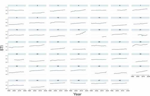
Table 6 shows that LDCs have more natural resources than NICs since the average per capita arable land in LDCs is 0.961 hectare compared to 0.0158 hectare in NICs. NICs have a more open economy since their trade openness is 213.80, which is more than four times that of LDCs (51.28 percent). In NICs, urban regions account for more than 87.99 percent of the population, but in LDCs, urban areas account for just 42.32 percent of the overall population. As a result, NICs’ per capita income (24,814 USD) is over ten times more than that of LDCs (2500 USD). Figure (3) illustrates the significant disparity between NIC and LDC per capita income as well as the alarmingly rapid increase of NCI relative to LDC. (Figure 4) shows the evolution of structural transformation from 1990 to 2018, based on each country’s estimated STI. In the chosen developing countries, structural transformation has improved by 20.8 percent, from 0.3930 in 1990 to 0.4749 in 2018. However, between 1990 and 2018, the structural transformation of NICs improved by 7.05 percent, from 0.8008 to 0.8573. In comparison to developing countries, NICs have made less progress in structural transformation since they have nearly hit the saturation point of structural transformation in the 1990s. The slope of their graph in (Figure 4), as indicated in numbers 45, 46, 47, and 48, is virtually flat, indicating minimal structural transformation during the study period. According to (Figure 4), the rate of structural transformation in Cambodia, Vietnam, and China is alarming; on the other hand, Ethiopia has shown very modest progress in structural transformation during the study period, while structural transformation development in Lesotho has been unpredictable.

Table 6. Descriptive statistics

Variables		LDCs	NICs	Variables	LDCs	NICs
Value-Added Share (%)	Agriculture	18.67	1.58	Manufacturing Export (%)	44.97	87.23
	Manufacturing	16.27	21.31	FDI-GDP (%)	24.09	135.67
	Industry	23.90	28.38	Per Capita CA (‘000 USD)	227.38	323.97
	Services	37.02	49.67	Per capita GDP (USD)	2500	24,814
Employment share (%)	Agriculture	46.06	4.37	Per Capita Arable land (ha)	0.961	0.0158
	Manufacturing	10.39	19.09	Openness of Trade (%)	51.28	213.80
	Industry	25.78	28.64	Urbanization (%)	42.32	87.99
	Services	22.15	41.14	Human Capital Index	2.02	3.00

LDCs are all 44 developing countries, ha = hectare, USD = USA dollar.

Figure 4. Trends of structural transformation (1990–2018).

Note: 1 = Argentina, 2 = Burkina Faso, 3 = Bangladesh, 4 = Bolivia, 5 = Brazil, 6 = Botswana, 7 = China, 8 = Cameroon, 9 = Colombia, 10 = Costa Rica, 11 = Ecuador, 12 = Egypt, 13 = Ethiopia, 14 = Ghana, 15 = Indonesia, 16 = India, 17 = Kenya, 18 = Cambodia, 19 = LAOs, 20 = Sri Lanka, 21 = Lesotho, 22 = Morocco, 23 = Mexico, 24 = Myanmar, 25 = Mozambique, 26 = Mauritius, 27 = Malawi, 28 = Malaysia, 29 = Namibia, 30 = Nigeria, 31 = Nepal, 32 = Pakistan, 33 = Peru, 34 = Philippines, 35 = Rwanda, 36 = Senegal, 37 = Thailand, 38 = Tunisia, 39 = Turkey, 40 = Tanzania, 41 = Uganda, 42 = Viet Nam, 43 = South Africa, 44 = Zambia, 45 = Taiwan, 46 = Hong Kong, 47 = South Korea, and 48 = Singapore.

4.2. Econometric analysis

The econometric analysis is the second portion of the result and discussion section. To accomplish so, we first provided the various tests necessary to perform regression.

When the data is imbalanced, the Fisher-type unit root test is appropriate (Choi, 2001), with the null hypothesis that all panels have a unit root as the null hypothesis. The null hypothesis was rejected, as shown in Table 7, indicating that our data is not affected by the unit root problem. The Arallano-Bond (1991) estimation test for zero autocorrelation in first-differenced error (null hypothesis: no autocorrelation) for first-order serial correlation is rejected (z = −3.0139 with p-value = 0.0026) but not for second-order serial correlation (because p-value = 0.1972 is greater than the critical value = 0.05) implies that the Arallano-Bond estimation is free from second-order serial correlation. With a p-value of 0.184, the Sargan test of over-identification restriction test failed to reject the null hypothesis that over-identification restrictions are valid.

Table 7. Fisher unit root test

	Inverse chi-square (P)		Inverse Normal (Z)		Inverse Logit (L)		Modified inv.Chi-squared (Pm)
	Statistic	p-value	Statistic	p-value	Statistic	p-value	Statistic	p-value
lnSTI	313.994	0.0000	−10.4827	0.0000	−11.9114	0.0000	17.035	0.0000
lnFDI	264.784	0.0000	−7.9431	0.0000	−9.4379	0.0000	13.325	0.0000
lnAL	215.262	0.0000	−7.0131	0.0000	−7.5376	0.0000	9.5928	0.0000
lnOT	285.015	0.0000	−10.9793	0.0000	−11.5289	0.0000	14.850	0.0000
lnPoP	1461.85	0.0000	−25.8815	0.0000	−54.8006	0.0000	103.55	0.0000
lnPcGDP	120.168	0.0129	−2.7038	0.0034	−2.5133	0.0063	2.4248	0.0077
lnCA_GDP	226.359	0.0000	−7.8688	0.0000	−8.1571	0.0000	10.429	0.0000
lnHC	695.269	0.0000	−5.9966	0.0000	−13.1849	0.0000	45.774	0.0000
lnMVA	212.674	0.0000	−7.5378	0.0000	−7.7980	0.0000	9.3977	0.0000
lnSVA	273.452	0.0000	−10.1586	0.0000	−10.7595	0.0000	13.979	0.0000
lnMEm	284.147	0.0000	−8.7327	0.0000	−10.6896	0.0000	14.785	0.0000
lnSE	264.920	0.0000	−7.1087	0.0000	−8.7091	0.0000	13.335	0.0000
lnMEXP	398.256	0.0000	−13.6284	0.0000	−16.2213	0.0000	23.386	0.0000
lnUP	1064.78	0.0000	−17.7602	0.0000	−36.6276	0.0000	73.627	0.0000

According to Table 8, ceteris paribus, a percentage increase in FDI stock raises the amount of structural transformation by 0.0214 percent on average. Furthermore, given the estimated persistence of structural transformation (i.e. lnSTIt-1), the long-run effect on a percentage increase in FDI stock is estimated to be 0.0626 percent (coefficient of lnSTIt-1/ (1-cofficient of lnFDI). It supports the argument that FDI promotes the domestic economy by inducing resource reallocation from less-productive to high-productive sectors, increasing domestic firm productivity by learning about new production techniques and management practices, acquiring technology and knowledge of international markets and trade, and creating linkage (backward) to the domestic economy. This finding is consistent with the findings of Mensah et al. (2016), Topcu (2016), Montes and Cruz (2020), Jie and Shamshedin (2019), Thirion (2020), and Muhlen and Escobar (2020) who all found that FDI affects structural transformation positively in developing countries by bringing capital investment, cutting-edge technology, and new skills. The result of this study, however, contradicts the findings of Aitken and Harrison (1999), Gui-Diby and Renard (2015), Samouel and Aram (2016), Chenaf-Nicet (2019), Maroof et al. (2019), and Oduola et al. (2022) who concluded that FDI did not contribute to structural transformation in developing countries due to ineffective government interventions, inability to create an enabling environment for FDI, market-stealing effect and crowding-out of local firms, negative effect on productivity of local firms, inflows of resource-seeking dominated FDI, and repatriation of profits.

Table 8. The one-step arallano-bond (1991) estimation output (Developing Countries)

lnSTI	Coefficient	Robust Std.Err.	Z	P>/z/	[95% Conf. Interval]
lnSTIt-1	0.6581***	0.0666	9.88	0.000	0.5274683	0.7886619
lnFDI	0.0214***	0.0079	2.71	0.007	0.0058955	0.0368593
lnAL	0.1370***	0.0582	2.35	0.019	0.0229704	0.2511151
lnOT	0.2007	0.0213	0.94	0.345	−0.0216174	0.061759
lnPoP	0.0461	0.0534	0.86	0.389	−0.0586279	0.1507366

All of the control variables have a beneficial effect on structural transformation, but only the initial condition (STIt-1) and arable land have a statistically significant effect. We concentrated on significant variables because there was no need for explanations for negligible ones. The initial status of structural transformation (characterized by physical & human capital accumulation, structural changes, and economic growth) serve as fuel for further structural transformations. Improvements of one percent on initial structural transformation status result in a 0.66 percent further rise in structural transformation. In terms of arable land size, the structural transformation increases by about 0.14 percent for every percentage point increase in arable land size, ceteris paribus. Increasing the size of arable land by 1 percent increases structural transformation by 0.76 percent (coefficient of lnSTIt-1/ (1-coefficient of lnAL). This empirical finding is in agreement with Gui-Diby and Renard (2015), who observed that vast areas of arable land could produce agricultural products, which could generate the raw materials for industry sectors and the necessary capital to enable industrialization. Our result is also in line with that of Ren et al. (2019), which provides empirical evidence that a large arable land size promotes agricultural modernization which is at the core of structural transformation in developing countries via promotimg the large-scale farming, agricultural cooperation in production and sales, and mechanized farming. This finding disproves Feder’s (1985) assertion that large farms tend to use hired labor more intensively than small farms, resulting in less productivity per unit land, which is a prerequisite for structural transformation, compared with smaller plots.

Since FDI contributes positively to developing countries’ structural transformation, how it influences structural transformation is an important subject that must be addressed in this section. As previously said, it is influenced primarily through three channels: per capita income growth, capital accumulation, and structural changes. To keep the size of this article manageable, we focused only on the structural change channel to examine the relationship between FDI and structural transformation.

Table 9 shows that FDI inflows have a positive and significant effect on manufacturing value-added. Ceteris paribus, a one percentage point rise in FDI stock results in a 1.56 percent increase in manufacturing value-added production. Our findings are consistent with past works presented by Timothy and Chigozie (2015), Anyanwu (2017), and Saif-ur and Abu (2019) which suggest that FDI is crucial for the transformation of the manufacturing sector by providing additional capital, facilitating forward and backward links, transferring technology and knowledge, and creating additional capital through high employment utilization. It contradicts the findings by Mamba et al. (2020) in WAEMU, which claim that FDI fails to promote industrialization as a result of insufficient incentives to attract FDI to the manufacturing sector. It also inconsistencies with the findings of Muller (2021), which show that FDIs have a highly significant negative effect on the industrialization of SSA countries due to the fact of FDI inflows that are driven by corruption and that are dominated by the primary sector, as well as relatively weak institutional qualities like poor governance and difficulty doing business in FDI-receiving countries. As to employment, our empirical evidence suggests FDI has a significant positive effect on manufacturing employment. If all other factors stay the same, every 1 percent increase in FDI stock increases the manufacturing employment share of total employment by 0.077 percent. This suggests that FDI in the manufacturing sector makes extensive use of both skilled and unskilled labor, as well as the creation of numerous small and medium-sized manufacturing enterprises with the capacity to absorb huge amounts of labor through backward linkages. This result is consistent with the majority of earlier research findings, including Waldkirch et al. (2009) and Saucedo et al. (2020). In terms of promoting manufacturing exports, our empirical evidence indicates that FDI has no substantial influence on increasing the share of manufacturing exports in merchandise exports. This could imply that FDI in developing nations is resource-seeking, which increases raw material exports, or market-seeking, which increases dampening of MNEs’ products in host countries.

Table 9. Fixed effect model estimation output (Developing Countries)

Variables	Output		Labor shift		Manufacturing Export	Urbanization
	lnMVA	lnSVA	lnMEm	lnSE
lnFDI	0.0156* (0.0091)	0.0236*** (0.0048)	0.0766** (0.0124)	0.0232*** (0.0083)	−0.0125 (0.0244)	0.0335**** (0.0048)
lnPcGDP	0.0096 (0.0205)	0.0287*** (0.0108)	−0.0253 (0.0279)	0.0577*** (0.0187)	−0.1672*** (0.0502)	0.0297*** (0.0108)
lnCA_GDP	0.1550*** (0.0163)	0.0378*** (0.0086)	−0.069*** (0.0221)	0.0064 (0.0148)	−0.0798** (0.0389)	−0.0047*** (0.0086)
lnHC	−0.2401** (0.1047)	0.2141*** (0.0551)	−0.854*** (0.1427)	0.0133 (0.0956)	1.0965*** (0.2515)	0.0940* (0.0552)
lnAL	0.0930** (0.0373)	0.1016*** (0.0196)	0.3442*** (0.0508)	0.2824*** (0.0340)	0.0960 (0.0902)	0.1465*** (0.0196)
lnOT	−0.0161 (0.0224)	−0.0068 (0.0118)	0.2333*** (0.0305)	0.0925*** (0.0205)	0.0071 (0.0555)	−0.0091 (0.0118)
lnPoP	−0.3590*** (0.0644)	−0.1308*** (0.0339)	0.1805*** (0.0877)	0.8977*** (0.0588)	0.2422 (0.1633)	0.3103*** (0.0339)
Hausman test	X^2 = 82.15 P = 0.000	X^2 = 32.91 P = 0.000	X^2 = 144.6 P = 0.000	X^2 = 260.1 P = 0.000	X^2 = 116.46 P = 0.0000	X^2 = 104.29 P = 0.0000
F-test	F = 126 P = 0.000	F = 70.35 P = 0.000	F = 105.3 P = 0.000	F = 82.76 P = 0.000	F = 146.85 P = 0.000	F = 315.68 P = 0.0000

MVA = the share of manufacturing value added in total value-added output, MEm = share of manufacturing employment in total employment, SE = share of services employment, MEx = share of manufacturing export in total merchandise export, ln = natural logarithm, X² = chi-square, P = probability, and F = F-value. The sign *, **, and *** indicates it is significant at 10, 5, and 1 percent significance level, respectively. Standard errors are reported in parentheses.

Similarly, FDI has a favorable and considerable effect on the value-added production and employment in the services sector. According to Table 9, all factors remain constant; a percentage increase in FDI stock generates a 2.36 percent and a 2.32 percent rise in the service sector’s share of total production and employment, respectively. This suggests that FDI in the service sector by itself, as well as FDI in other sectors like agriculture, mining, manufacturing, and construction, need services like transportation, banking, communication, hotels, and other commercial services; as a result, FDI has a significant ability to stimulate production and employment in the service sector. According to structural change theories such as Chenery (1960), increasing the share of service sector employment is normal because it should exhibit a steady growth from the early stage of transformation to the final stage. It is also in line with the empirical output found by Mamba et al. (2020) in WAEMU. It conflicts with the SSA conclusion made by Muller (2021). Finally, our empirical evidence reveals that FDI is vital for structural transformation in developing countries via facilitating urbanization. As shown in Table 9, all things remain the same; a percentage rise in FDI stock correlates with a 0.034 percent rise in urbanization. This supports the findings of Mamba et al. (2020) in WAEMU stating FDIs are usually concentrated in metropolitan areas (to reduce transportation and communication expenses and weak infrastructure in rural regions), with better incentives for employees to move from rural to urban areas. This is also consistent with Foldi and Weesep’s (2006) and Wu and Zhao’s (2019) findings, which found FDI altered people’s lifestyles, changing urban cultures and resulting in urbanization, as well as promoting economic expansion, which also leads to urbanization.

5. Conclusion remarks

Structural transformation is crucial, but it is still difficult to achieve in developing countries due to low domestic resources, a lack of technology and managerial expertise, and a low development of the industrial sector to lead it. FDI is a critical factor in structural transformation; yet, study on this issue has been limited, particularly in developing countries. Thus, this study examined the effect of FDI on structural transformation in 44 developing countries from Africa, Latin America, and Asia, selected based on data accessible from 1990 to 2018. According to the analysis, structural transformation has been less successful in Africa, particularly Sub-Saharan Africa, despite Asia’s relative performance. The results of Arellano-Bond (1991) suggest that FDI inflows promote structural transformation. Moreover, the paper explores the channels through which FDI affects structural transformation. Based on the Principal Component Analysis, structural change is primarily responsible for structural transformation, followed by capital accumulation, and then by economic growth. As structural change indicators such as manufacturing output and employment, service-sector output and employment, and urbanization are important channels through which FDI promotes structural transformation in developing countries, whereas manufacturing exports have an adverse but negligible effect.

Similarly, different control variables, such as initial structural transformation status and arable land size, play significant roles in facilitating structural transition in developing countries. Because empirical research suggests that FDI promotes both manufacturing production and employment in developing countries, policymakers in developing countries should stress this in their FDI attractiveness policies. They should also encourage policies that faciliate labor mobility to petentially increase the effects of FDI on structural transformation. Manufacturing-export motivated FDI, in particular, should be encouraged in policy by introducing specific incentives such as tax and tariff exemptions, land and infrastructure provision, and less bureaucracy for them. Improving host countries’ absorptive ability by, for example, enabling domestic enterprises to acquire technology from foreign firms by giving financial access and training opportunities, and improving human capital acummulation by, at the very least, supporting technical and vocational education. Moreover, as population pressure causes agricultural landholdings per capita to decrease over time, governments in these countries should encourage farmers to consolidate their land by providing various incentives, such as allowing the commercial sale of land, in order to achieve agricultural-sector transformation, which is a necessary condition for structural transformation.

Disclosure statement

No potential conflict of interest was reported by the author(s).

Additional information

Funding

The authors received no direct funding for this research.

Notes on contributors

Ezo Emako

Ezo Emako is a PhD candidate in development economics at Arba Minch University in Ethiopia. Seid Nuru (PhD) is an associate professor of Economics. He is a lecturer and researcher at Arba Minch university. Mesfin Menza (PhD) is a lecturer, researcher, and dean of the Business and Economics College at Arba Minch University.

References

- Abdi, H., & Williams, L. J. (2010). Principal component analysis. Wiley Interdisciplinary Reviews: Computational Statistics, 2(4), 433–23. https://doi.org/10.1002/wics.101.
- Aitken, B. J., & Harrison, A. E. (1999). Do domestic firms benefits from direct foreign investment? Evidence from Venezuela. American Economic Review, 89(3), 605–618. https://doi.org/10.1257/aer.89.3.605
- Aksu, G., Duzeller, C. O., & Eser, M. T. (2019). The effect of the normalization method used in different sample sizes on the success of artificial neural network model. International Journal of Assessment Tools in Education, 6(2), 170–192. https://doi.org/10.21449/ijate.479404
- Alavin, M., Visentin, D. C., Thapa, D. K., Hunt, G. E., Watson, R., & Clearly, M. (2020). Explanatory factor analysis and principal component analysis in clinical studies: Which one should you use? Journal of Advanced Nursing, 76(8), 1886–1889. https://doi.org/10.1111/jan.14377.
- Anyanwu, J. C. (2017). Manufacturing value-added development in North Africa: Analysis of key drivers. Asian Development Policy Review, 5(4), 281–298. https://doi.org/10.18488/journal.107.2017.54.281.298
- Awaliyyah, E. Z., Chen, S., & Anindita, Suhartini, R. A. (2020). Analysis of structural transformation of labor from agriculture to non-agriculture in Asia. Agricultural Socio-Economics Journal, 20(4), 335–341. https://doi.org/10.21776/ub.agrise.2020.20.4.9
- Bah, E.-H. M. (2011). Structural transformtion paths across countries. Emerging Markets Finance & Trade, 47(sup2), 5–19. https://doi.org/10.2753/REE1540-496X4703S201
- Bauman, K., & Chenoweth, R. L. (1984). The relationship between the consequences adolescents expect from smoking and their behavior: A factor analysis with panel data. Journal of Applied Aocial Psychology, 14(1), 28–41. https://doi.org/10.1111/j.1559-1816.1984.tb02218.x.
- Chenaf-Nicet, D. (2019). Dynamic of structural change in globalized world: What is the role played by institutions in the case of Sub-Saharan African Countries. The Eropean Journal of Development Research 32, 998–1037. https://doi.org/10.1057/s41287-019-00250-2.
- Chenery, H. B. (1960). Patterns of industrial growth. The American Economic Review, 50(4), 624–654. https://www.jstor.org/stable/1812463.
- Chenery, H., Robinson, S., & Syrquin, M. (1986). Industrialization and growth: A comparative study. Published for the World Bnak [by] Oxford University Press.
- Chenery, H., & Syrquin, M. (1975). Patterns of development, 1950-1970. Oxford University Press.
- Chenery, H. B., & Taylor, L. (1968). Development patterns: Among countries and over time. The Review of Economics and Statistics, 50(4), 391–416. https://doi.org/10.2307/1926806
- Choi, I. (2001). Unit root test for panel data. Journal of International Money and Finance, 20(2), 249–272. https://doi.org/10.1016/S0261-5606(00)00048-6
- Domar, E. (1947). Expansion and employment. American Economic Review, 37 1 , 34–55 http://www.jstor.org/stable/1802857.
- Duarte, M., & Restuccia, D. (2010). The role of the structural transformation in aggregate productivity. The Quarterly Journal of Economics, 125(1), 129–173. https://doi.org/10.1162/qjec.2010.125.1.129
- Faruqi, R., & O’Brien, P. (1976). Foreign technology in the growth of the modern manufacturing sector in Ethiopia 1950-1970. Africa Development/Afrique et Développement, 1(2), 23–43 https://www.jstor.org/stable/44898430.
- Feder, G. (1985). The relationship between farm size and farm productivity: The role of family labor, supervision, and credit constraints. Journal of Development Economics, 18(2–3), 297–313. https://doi.org/10.1016/0304-3878(85)90059-8
- Foldi, Z., & Weesep, J. (2006). Impacts of globalization at the neighborhood-level in Budapest. Journal of Housing and the Built Environment, 22(1), 33–50. https://doi.org/10.1007/s10901-006-9065-2
- Fukase, E. (2010). Revising linkages between openness, education and economic growth: System GMM approach. Journal of Economic Integration, 25(1), 193–222. https://doi.org/10.11130/jei.2010.25.1.194
- Granato, D., Santos, J. S., Escher, G. B., Ferreira, B. L., & Maggio, R. M. (2018). Use of Principal Component Analysis (PCA) and Hierarchical Cluster Analysis (HCA) for multivariate association between bioactive compounds and functional properties in foods: A critical perspective. Trends in Food Science and Technology, 72, 83–90. https://doi.org/10.1016/j.tifs.2017.12.006
- Greene, W. H. (2003). Econometric analysis (1st ed.). New York University.
- Gui-Diby, S. L., & Renard, M. (2015). Foreign direct investment inflows and the industrialization of Africa Countries. World Development, 74, 43–57. https://doi.org/10.1016/j.worlddev.2015.04.005.
- Gujarati, D. N. (2003). Basic econometrics (4th ed.). MCGrow-Hill Higher Education.
- Gygli, S., Haelg, F., Potrafke, N., & Sturm, J. (2019). The KOF globalisation index - revisited. The Review of International Organizations, 14(3), 543–574. https://doi.org/10.1007/s11558-019-09344-2
- Hajkowicz, S. (2006). Multi-attribute environmental index construction. Ecological Economics, 57(1), 122–139. https://doi.org/10.1016/j.ecolecon.2005.03.023
- Harrod, R. F. (1939). An essay in dynamic theory. Economic Journal, 49(193), 14–33. https://doi.org/10.2307/2225181
- Hauge, J. (2019). Should the Africab Lion from the Asian tigers? A Comparative-historical study of FDI-oreinted industrial policy in Ethiopia, South Korea and Taiwan. Third World Quarterly, 40(11), 2071–2091. https://doi.org/10.1080/01436597.2019.1629816
- Iezzoni, A. F., & Pritts, M. P. (1991). Applications of principal component analysis to horticultural research. HortScience, 26(4), 334–338. https://doi.org/10.21273/HORTSCI.26.4.334
- Jie, L., & Shamshedin, A. (2019). The impact of FDI on industrialization in Ethiopia. International Journal of Academic Research in Business and Social Sciences, 9(7), 726–742. https://doi.org/10.6007/IJARBSS/v9-i7/6175
- JRCEC (2005). Tools for composite indicators building. http://europa.eu.int
- Khan, M. A. (2020). Cross sectoral linkage to explain structural transformation in Nepal. Structural Change and Economic Dynamics, 52, 221–235. https://doi.org/10.1016/j.strueco.2019.11.005
- Kinnunen, J., Androniceanu, A., & Georgescu, I. (2019). The role of economic and political features in classification of countries-in-transition by human development index. Informatica Economică, 23(4), 26–40. https://doi.org/10.12948/14531305/23.4.2019.03
- Kuznets, S. (1966). Modern growth and structure. Yale University Press.
- Kuznets, S. (1973). Modern economic growth: Findings and reflections. The American Economic Review, 63(3), 247–258 http://www.jstor.org/stable/1914358.
- Lewis, W. A. (1954). Economic development with unlimited supplies of labour. The Manchester School, 22(2), 139–191. https://doi.org/10.1111/j.1467-9957.1954.tb00021.x
- Mamba, E., Ginigue, M., & Ali, E. (2020). Effect of foreign direct investment on structural transformation in West African Economic and Monetary Union (WAEMU) Countries. Cogent Economics & Finance, 8(1), 1–21. https://doi.org/10.1080/23322039.2020.1783910
- Marjanovic, V. (2015). Structural challenges and structural transformation in a modern development economy. Economic Themes, 53(1), 63–82. https://doi.org/10.1515/ethemes-2015-0005
- Maroof, Z., Hussain, S., Jawad, M., & Naz, M. (2019). Determinants of industrial development: A panel analysis of South Asian economies. Quality & Quantity, 53(3), 1391–1419. https://doi.org/10.1007/s11135-018-0820-8
- McMillan, M., & Headey, D. (2014). Introduction - understanding structural transformation in Africa. World Development, 63, 1–10. https://doi.org/10.1016/j.worlddev.2014.02.007
- McMillan, M., Rodrik, D., & Verduzco-Gallo, I. (2014). Globalization, structural change, and productivity growth with an unpdate on Africa. World Development, 63, 11–32. https://doi.org/10.1016/j.worlddev.2013.10.012.
- Mensah, J. T., Adu, G., Amoah, A., Abrokwa, K. K., & Adu, J. (2016). What drives structural transformation in Sub-Saharan Africa? African Development Review, 28(2), 157–169. https://doi.org/10.1111/1467-8268.12187
- Mohamad, M., Juahir, H., Ali, N. A. M., Kamarudin, M. K. A., Karim, F., & Badarilah, N. (2017). Developing health status index using factor analysis. Journal of Fundamental and Applied Sciences, 9(2S), 82–92. https://doi.org/10.4314/jfas.v9i2s.6
- Montes, M. F., & Cruz, J. (2020). The political economy of foreign investments and industrial development: The Philippines, Malaysia, and Thailand in comparative perspective. Journal of the Asian Pacific Economy 25 1 , 16–39. https://doi.org/10.1080/13547860.2019.1577207
- Moral-Benito, E., Allison, P., & Williams, R. (2018). Dynamic panel data modelling using maximum likelihood: An alternative to arellano-bond. Applied Economics 51(20), 2221–2232. https://doi.org/10.1080/00036846.2018.1540854.
- Muhlen, H., & Escobar, O. (2020). The role of FDI in structural change: Evidence from Mexico. World Economy, 43(3), 557–585. https://doi.org/10.1111/twec.12879
- Muller, P. (2021). Impacts of inward FDIs and ICT penetration on the industrialisation of Sub-Saharan African Countries. Structural Chnage and Economic Dynamics, 56, 265–279. https://doi.org/10.1016/j.strueco.2020.12.004
- Oduola, M., Bello, M. O., & Popoola, R. (2022). Foreign direct investment, institution and industrialisation in Sub-Saharan Africa. Economic Change and Restructuring, 55, 577–606. https://doi.org/10.1007/s10644-021-09322-y.
- Olawale, F., & Garwe, D. (2010). Obstacles to the growth of new SMEs in South Africa: A principal component analysis approach. African Journal of Business Management, 4(5), 729–738 https://academicjournals.org/article/article1380715803_Olawale%20and%20Garwe.pdf.
- Ranis, G., & Fei, J. C. H. (1961). A theory of economic development. American Economic Association, 51(4), 533–565 http://www.jstor.org/stable/1812785.
- Ren, C., Liu, S., van Grinsven, H., Reis, S., Jin, S., Liu, H., & Gu, B. (2019). The impact of farm size on agricultural sustainability. Journal of Cleaner Production, 220, 357–367. https://doi.org/10.1016/j.jclepro.2019.02.151
- Rodrik, D. (2018). An African growth miracle? Journal of African Economies, 27(1), 10–27. https://doi.org/10.1093/jae/ejw027.
- Romer, P. M. (1990). Endogenous technological change. Journal of Political Economy, 98(5), S71–S102. https://www.jstor.org/stable/2937632.
- Rostow, W. W. (1956). The take-off into self-sustained growth. The Economic Journal, 66(261), 25–48. https://doi.org/10.2307/2227401
- Rostow, W. W. (1959). The stages of economic growth. The Economic History Review, 12(1), 1–16. https://doi.org/10.1111/j.1468-0289.1959.tb01829.x
- Saif-ur, R., & Abu, B. N. (2019). FDI and manufacturing growth: Bound test and ARDL approach. International Journal of Research in Social Sciences, 9(5), 36–91. https://www.ijmra.us/project%20doc/2019/IJRSS_MAY2019/IJMRA-15391.pdf.
- Samouel, B., & Aram, B. (2016). The determinants of industrialization: Empirical evidence for Africa. European Scientific Journal, Special Edition 12(10) , 219–239. https://doi.org/10.19044/esj.2016.v12n10. .
- Saranya, C., & Manikandan, G. (2013). A study on normalization techniques for privacy presenting data mining. International Journal of Engineering and Technology (IJET), 5(3), 2701–2704 https://citeseerx.ist.psu.edu/viewdoc/download?doi=10.1.1.411.1996&rep=rep1&type=pdf.
- Saucedo, E., Jr, T. O., & Zamora, H. (2020). The effect of FDI on low and high-skilled employment and wages in Mexico: A study for the manufacturing and service sectors. Journal of Labour Market Research, 54(9), 1–15. https://doi.org/10.1186/s12651-020-00273-x
- Shrestha, N. (2021). Factor analysis as a tool for survey analysis. American Journal of Applied Mathematics and Statistics, 9(1), 4–11. https://doi.org/10.12691/ajams-9-1-2
- Suleman, A. (2009). Fostering FDI in the agriculture sector. The Pakistan Development Review, 48(4), 821–838 https://www.jstor.org/stable/41261349.
- Syrquin, M. (2010). Kuznets and Pasinetti on the study of structural transformation: Never the twain shall meet? Structural Change and Economic Dynamics, 21(4), 248–257. https://doi.org/10.1016/j.strueco.2010.08.002
- Syrquin, M., & Chenery, H. (1989). Three decades of industrialization. The World Bank Economic Review, 3(2), 145–185. https://doi.org/10.1093/wber/3.2.145
- Teixeira, A. A. C., & Queiros, A. S. S. (2016). Economic growth, human capital and structural change: A dynamic panel analysis. Research Policy, 45(8), 1636–1648. https://doi.org/10.1016/j.respol.2016.04.006
- Thirion, J. M. (2020). FDI, regional development and structural change; The case of three states in El Bajio, Mexico. Analysis Economico, 35(90), 199–220 https://www.scielo.org.mx/scielo.php?pid=S2448-66552020000300199&script=sci_abstract&tlng=en.
- Timmer, C. P., & Akkus, S. (2008). Patterns of growth and structureal transformation in Africa Center for Global Development . https://www.files.ethz.ch
- Timothy, O. T., & Chigozie, A. O. (2015). Foreign direct investment flows and manufacturing sector performance in Nigeria. International Journal of Economics, Commerce and Management, 3(7), 412–428 https://ijecm.co.uk/wp-content/uploads/2015/07/3727.pdf.
- Topcu, B. A. (2016). The relationship between foreign direct investment and industrialization in developing countries: Panel data analysis. The Journal of Academic Social Science, 4(35), 390–400. https://doi.org/10.16992/asos.11631.
- Uy, T., Yi, K., & Zhang, J. (2013). Structural change in an open economy. Journal of Monetary Economics, 60(6), 667–682. https://doi.org/10.1016/j.jmoneco.2013.06.002
- Waldkirch, A., Nunnenkamp, P., & Bremont, J. E. A. (2009). Employment effects of FDI in Mexico’s non-maquiladora manufacturing. Journal of Development Studies, 45(7), 1165–1183. https://doi.org/10.1080/00220380902952340
- Watkins, M. W. (2018). Exploratory factor analysis: A guide to best practice. Journal of Black Psychology, 44(3) , 219–246. https://doi.org/10.1177/0095798418771807.
- Wu, W., & Zhao, K. (2019). Dynamic interaction between foreign direct investment and the new urbanization in China. Journal of Housing and the Built Environment, 34(4), 1107–1124. https://doi.org/10.1007/s10901-019-09666-y
- Yong, A. G., & Pearce, S. (2013). A beginner’s guide to factor analysis: Focusing on Exploratory factor analysis. Tutorials in Quantitative Methods for Psychology, 9(2), 79–94. https://doi.org/10.20982/tqmp.09.2.p079