A DSGE model of fiscal stabilizers and informality in Sub-Sahara Africa

Abstract

This paper investigates the effects of fiscal impulses on macroeconomic variables within a New-Keynesian DSGE framework featuring an informal economy that allows for the examination of the effectiveness of automatic stabilizers in stimulating some selected sub-Saharan African (SSA) economies during crises. Stabilizers were modelled such that fiscal instruments react to their own lagged values and the official sector output. The results indicate that tax hikes lead to sizeable tax evasion and reallocation of factor inputs from the official sector to the shadow sector making the standard aggregate estimates of fiscal policies ineffective while government spending shocks slow down activities in the shadow sector. The findings also showed that automatic stabilizers on government spending (income taxes) stabilized the economy by reducing (raising) output levels even in the presence of the shadow economy. For policy implications, effective implementation of government policies should incorporate the informal sector in macroeconomic modelling, especially for countries with a large informal sector.

Keywords:

• Fiscal policy
• automatic stabilizers
• informality
• DSGE models
• Sub-Sahara Africa

JEL codes:

• D58
• E12
• E26
• E52
• E62

1. Introduction

Automatic fiscal stabilizers have become an important feature of macroeconomic modelling given its role in stimulating the economy. These measures gained further credence during the global financial and economic crisis whereby fiscal policy became the ultimate stimuli response. The paradigm shift was due to the inability of monetary policy to avoid the recession making fiscal tools an important topic in the macroeconomic modelling process. Following this, fiscal expansion became large in the advanced countries such as the US and the UK while many governments in the Euro area were criticized by the IMF for taking slow actions in the 2007–2009 period and for “austerity” measures imposed on peripheral countries after the beginning of the Greek crisis in 2010 (Krugman, 2012; Stiglitz et al., 2014). As suggested by Magazzino (2022); Magazzino and Mutascu (2022), there are no acceptable empirical criteria for judging fiscal sustainability programs. However, the key definition is based on the intertemporal budget constraint of the state, according to which public finances are sustainable if the present value of all future government revenues is at least equal to the present value of all future expenditure, plus the initial value of the debt. The recent global crisis caused by the COVID-19 pandemic has resulted in an unprecedented decline in global economies’ GDP of which Africa is no exception. In view of this, most governments around the world and Sub-Sahara Africa provide support to the most affected sectors of the economy to spur economic recovery. Governments reacted by increasing public deficits which, between discretionary measures and automatic stabilizers, reached the highest levels since the Second World War. This has called for prudent fiscal macroeconomic policies that would result in fiscal sustainability. The current study focuses on how sub-Saharan African countries have responded to this crisis using one of the conventional macroeconomic measures of fiscal stabilizers (see, Magazzino, 2022; Magazzino & Mutascu, 2022).

Automatic stabilizers are conceptualized as budgetary arrangements that help to smooth output without the explicit intervention of the fiscal authority (Larch & Vandeweyer, 2013; McKay & Reis, 2016). Typically, automatic stabilizers are tax and transfer systems that temper the economy when it overheats and stimulates growth when it slumps without the direct involvement of policymakers. The recent COVID-19 pandemic and its related effects have necessitated the need to examine the effectiveness of automatic stabilizers in stimulating economies. Policy options for stabilizing the economy in the wake of a crisis can be discretionary or automatic. However, there have been a lot of arguments that discretionary fiscal policy is often not effective in stabilizing the economy during a crisis. Discretionary fiscal policies are often found to be counter-productive given that implementation of lags in the crisis period is less important than during normal times (Colciago et al., 2008; Hemming et al., 2002; Larch & Vandeweyer, 2013; McKay & Reis, 2016; Taylor, 2009). The last decades have seen advancements in estimation methodology that is micro-founded and has particularly become suitable for evaluating the effects of alternative macroeconomic policies. Dynamic Stochastic General Equilibrium (DSGE) models have been known to provide coherent and consistent results in identifying the effectiveness of fiscal impulses.¹ This work, therefore, examines the role and effectiveness of automatic fiscal stabilizers in the presence of the shadow economy in SSA countries.

Informal production sectors constitute a greater proportion of economic activities in developing and emerging economies. For instance, Schneider et al. (2010) reported the size of the informal economy for 162 countries from 1999 to 2007. Figures 1a and b present the flow and trends of the share of informal sector activities as a percentage of GDP in some selected SSA countries.

Figure 1. A and b. share of shadow activities as a percentage of GDP in some selected SSA countries.

Source: Schneider et al. (2010).

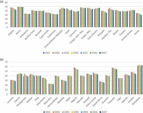
The data is taken from Schneider et al. (2010), who developed a methodology to calculate the size of the shadow sector in some 162 countries including some SSA countries. Latin America and the Caribbean top the list with 41.4% of GDP, closely followed by sub-Saharan Africa, 40.2%, and then by Eastern Europe and Central Asia, with the same percentages, 38.9%. Medina and Schneider (2018); Makochekanwa (2020), reported the size of informal economy for 49 African countries from 1991 through 2015. The studies showed that the size of the informal economy in Africa in terms of its contribution to GDP has declined from an average of 42% of total GDP in 1991 to 35% of total GDP by end of 2015. SSA countries that dominated include Zimbabwe with the highest level of informality contributing on average 61% towards the country’s GDP. The informal activity in Zimbabwe has grown from contributing 57% of annual GDP in 1991 to 67% of GDP in 2015. Nigeria came as the second-ranked country with high informality averaging 57% of the country’s GDP, though growth in this sector has declined from 1991 to 2015. On the other extreme, Mauritius is the country with the least informal economy averaging 23% of the national GDP. Informal economic activities in Mauritius have been decreasing from 26% of the country’s GDP in 1991 to 19% of its GDP in 2015. Additionally, Singh and Capt (2002), Nguimkeu and Okou (2019), and Makochekanwa (2020) indicated that street vending predominates in much of the informal economy in most parts of sub-Saharan Africa. Standard DSGE literature lacks the prerequisite modelling ingredients for developing and emerging countries which makes the adoption of such models for policymaking questionable. Developing countries are typically characterized by a weak financial sector, the existence of a large informal sector, external shock vulnerability, and weak economic and political institutions. This study seeks to elucidate whether the presence of a shadow economy dampens or amplifies the effects of fiscal policy transmissions with automatic stabilizers. Secondly, we try to identify the role of alternative fiscal shocks and feedback on GDP by comparing the cases with and without a shadow economy.

We, therefore, perform this examination by allowing for fiscal stabilizers on government spending, labour and capital income taxes. Fiscal stability allows fiscal instruments to depend on the level of official sector output and it postulates that whenever the official output is below its long-run level, fiscal spending increases and income tax rates fall. The study imposes a stabilization policy and compares it with the model without fiscal stabilizers in both one-sector and two-sector models. The work then computes a fiscal gap variable for the two cases in each model.² Fiscal policy packages are computed as average effective tax rates on labour income, capital income and consumption tax following Melina et al. (2016) which are consistent with data collected by the International Bureau of Fiscal Documentation in 2005–06. On the expenditure side, we take into consideration the variable mostly used in the literature, that is the government consumption expenditure from national income data which includes both purchases of goods and services as well as compensations to employees as in Rotemberg and Woodford (1992).

The model is characterised by a competitive labour market where firms in both sectors pay the same consumption real wage. This assumption is motivated by the theoretical contributions from Amaral and Quintin (2006); Pratap and Quintin (2006) and supported by Maloney (1999, 2004). The contributions by Pratap and Quintin (2006) to developing countries provided evidence against labour market segmentation and suggested that labour market arguments are not necessary to account for the silent features of the labour market in developing countries. The model features real (adjustment cost in investment and utilization rate of capital) and nominal (price adjustment) frictions that appear to be necessary to capture the empirical persistence in the main macroeconomic data which have become quite standard in the DSGE literature. Smets and Wouters (2007) model exhibit both sticky nominal prices and wages that adjust following a Calvo mechanism but we deviate from that and model goods producer’s prices using Rotemberg (1982) model with full indexation of prices.³ Our model also incorporates a variable capital utilisation rate which tends to smooth the adjustment of the rental rate of capital in response to changes in output.

As in Smets and Wouters (2007), the cost of adjusting the utilization rate is expressed in terms of consumption goods whereas the cost of adjusting the capital stock is modelled as a function of changes in investment, rather than the level of investments. The model focuses on structural shocks that are asymmetric to the formal sector including government spending, labour income tax and capital income tax shocks. The assumption is that regulatory authorities have full control of the official sector. There is a central bank which formulates monetary policy and finally, the fiscal feedback rules are captured by introducing consumption tax, labour and capital income taxes which are used by the government to finance its expenditure. A drawback to this is that we do not consider all the countries in SSA on the grounds of data limitation. Additionally, we not explore the effects of financial institution since the financial market is generally underdeveloped.

The remainder of the paper is structured as follows, section 2 presents a brief empirical literature review, section 3 provides an overview of the model, while section 4 reports on the parameters and steady-state ratios used for calibrating the model and also presents the results. Finally, section 5 concludes the work.

2. Related literature review

The vast majority of DSGE literature has discussed the role and effects of fiscal policies on macroeconomic variables and their determination on the real business cycle. Kumhof and Laxton (2007) developed a very comprehensive model for the analysis of fiscal policies, which incorporates four non-Ricardian features. In their analysis of the effects of a permanent increase in the US fiscal deficits and debt, they found medium and long-term effects that differ significantly from those of liquidity-constrained agents. Furthermore, they find deficits to have a significant effect on the current account. The informal sector forms an integral part of many economies in the world and is of larger proportions in most developing and emerging economies. Few of the literature, such as Aruoba (2010), Batini et al. (2011), Colombo et al. (2016), and Asif Khan and Khan (2011) on the financial crisis and (Acosta et al., 2009; Annicchiarico & Cesaroni, 2018; Chatterjee & Turnovsky, 2018; Junior et al., 2020; Schneider et al., 2010), consider informality as part of the modelling process.

Pappa (2009) studied the transmission of fiscal shocks in the labour market by employing a prototype RBC and a New Keynesian model with a structural vector autoregressive (VAR) model and predicted that shocks to government consumption, investment and employment must raise output and deficit. In effect, shocks to government consumption and investment increased real wages and employment simultaneously, however, the dynamics of employment shocks were a mix. Other standard empirical versions of the New Keynesian DSGE model also typically predict a positive or at least no significant negative response of private consumption to government spending shocks (Fatas & Mihov, 2001; Gali & Perotti, 2003; Mountford & Uhlig, 2009; Perotti et al., 2007). Indeed, most of the literature that analyses the impact of fiscal policy on economic activities focuses mainly on the size and sensitivity of fiscal multipliers as in Cogan et al. (2010), Christiano et al. (2011), and Coenen et al. (2012) with the consideration of the shadow sector. Recent literature that studied fiscal policy issues with informality includes Junior et al. (2020), Annicchiarico and Cesaroni (2018), Chatterjee and Turnovsky (2018), Schneider et al. (2010), and Acosta et al., (2009).

Closer literature to this current study are Junior et al. (2020) and Annicchiarico and Cesaroni (2018), however this study’s main departure from Junior et al. (2020) is the way the informal sector is modelled in this study using an underground production sector activity. Junior et al. (2020) used informality in the labour market as a measure of informal activities. To do this, the paper extends Albonico et al. (2016) which departs from Smets and Wouters (2003, 2007) with an informal sector to ascertain how fiscal policy innovations are transmitted into the real sector. The automatic stabilizers are modelled with three fiscal instruments to react to their own lagged values and to the official sector output where the latter is thought to reflect the notion of automatic stabilizers. A more realistic treatment of fiscal policy suggests that the inclusion of fiscal stabilizers might be important in assessing the stability of the model (see recent contributions by Coenen et al., 2012, 2013; Albonico et al., 2016).

3. Theoretical framework and methodology

This section discusses the various representative agents that constitute the New Keynesian model. We build a new Keynesian DSGE model which fits 40 selected sub-Sahara African countries. These countries were selected given their similarities in economic structure and data availability. A list of the 40 countries whose averages were used for this study is presented in Table 1 in the appendices.

Table 1. Countries used for the study

List of Countries
Angola	Lesotho
Benin	Liberia
Botswana	Madagascar
Burkina Faso	Malawi
Burundi	Mali
Cabo Verde	Mauritania
Cameroon	Mauritius
Central African Republic	Mozambique
Chad	Namibia
Comoros	Niger
Congo, Dem. Rep.	Nigeria
Congo, Rep.	Rwanda
Cote d’Ivoire	Senegal
Eswatini	Sierra Leone
Ethiopia	South Africa
Gambia, The	Tanzania
Ghana	Togo
Guinea	Uganda
Guinea-Bissau	Zambia
Kenya	Zimbabwe

4. Households

There is a continuum of households of measure unity that supply labour services to firms. Households are made up of individuals who consume, work in both sectors of the economy and return the wages they earn to the household. Households supply the same amount of undifferentiated labour services to each sector of the economy thereby setting their real wages to the marginal rate of substitution between consumption and labour supplied. Their savings and investment are made through purchasing government bonds and supplying capital to sectoral goods producers. Following earlier contributions by Merz (1995) and Andolfatto (1996), household members are assumed to perfectly share the risk of sectoral consumption so individuals’ consumption decisions are the same and independent of their working conditions. The lifetime utility of representative agents is characterized by:

(1) $U_t^i=E_t\sum _{n=0}^{\mathrm{\infty }}{\beta }^n\left\{\mathrm{l}\mathrm{n}\left(c_{t+n}^i\right)-\chi \frac{l_t^{i\left(1+\varphi \right)}}{1+\varphi }\right\}$(1)

where superscript $i\in o,u$ denote official and unofficial sector variables respectively, $\chi$ is the parameter that regulates the disutility of work and $\varphi$ defines the Frisch elasticity of labour. For each sector, household members own goods producers, hold physical capital and choose their investment in both sectors. Households can increase the supply of rental services from capital by investing in additional capital taking into account the adjustment cost of capital. Their intertemporal budget constraint is⁴:

(2) $c_t+\frac{P_t^o}{P_t}{i}_t^o+\frac{P_t^u}{P_t}{i}_t^u+\frac{B_t}{P_t{R}_t{\epsilon }_t^{RISK}}=\frac{B_{t-1}}{P_t}+\frac{P_t^u}{P_t}\left[w_t^u{l}_t^u+r_t^{k,u}{u}_t^u{\bar{k}}_t^u-a\left(u_t^u\right){\bar{k}}_t^u+{\mathrm{\Pi }}_t^u\right]+\frac{P_t^o}{P_t}\left[\left(1-{\tau }_t^w\right)w_t^o{l}_t^o+\left(1-{\tau }_t^k\right)r_t^{k,o}{u}_t^o{\bar{k}}_t^o-\left(1-{\tau }_t^k\right)a\left(u_t^o\right){\bar{k}}_t^o+{\tau }_t^k\delta {\bar{k}}_t^o+{\mathrm{\Pi }}_t^o-T_t\right]$(2)

where $B_t$ is government bond that pays one unit of currency in period $t-1$ and $R_t$ is the gross nominal interest rate. We define sectoral variables: the relative goods prices $P_t^i$, the capital $k_t^i$ (where a bar on top of capital indicates physical units of capital), labour services $l_t^i$, the returns on capital $r_t^{k,i}$, the utilisation rate of capital $u_t^{\hspace{0.17em}}$, ${\mathrm{\Pi }}_t^i$ represent the profit received from investment in goods production and product wage $w_t^i$. The term $a\left(u_t^i\right)$ defines the real cost of using the capital stock with intensity $u_t^i$. The fiscal authority makes net lump-sum taxes $T_t$ which allows dealing with debt accumulation, and finances its expenditures by issuing bonds and by levying taxes on labour income ${\tau }_t^w$ and capital income ${\tau }_t^k$. Taxes are paid by those in the official sector only which is natural in modelling processes. ${\epsilon }_t^{RISK}$ is the risk premium shock on the returns to bonds that affects the intertemporal margin, creating a wedge between the interest rate controlled by the central bank and the return on assets held by the households, which follows an AR(1) stochastic process with an $i.i.d$ error term given as:

(3) $ln{\epsilon }_t^{RISK}={\rho }^{RISK}ln{\epsilon }_{t-1}^{RISK}+{\xi }_t^{RISK}$(3)

Households’ stock of physical capital in each sector is driven by the standard dynamic equation for capital given respectively as:

(4) ${\bar{k}}_{t+1}^o=\left(1-\delta \right){\bar{k}}_t^o+{\epsilon }_t^{INV}\left[1-S\left(\frac{i_t^o}{i_{t-1}^o}\right)\right]i_t^o$(4)

(5) ${\bar{k}}_{t+1}^u=\left(1-\delta \right){\bar{k}}_t^u+\left[1-S\left(\frac{i_t^u}{i_{t-1}^u}\right)\right]i_t^u$(5)

where $S\left(.\right)$ introduces the investment adjustment cost function.⁵ $\delta$ is the depreciation rate and only capital used in period $u_t^i{\bar{k}}_t^i$ is subject to depreciation. ${\epsilon }_t^{INV}$ is the stochastic shock⁶ to the price of investment relative to consumption goods and follows an exogenous process with an $i.i.d.$ error term as:

(6) $ln{\epsilon }_t^{INV}={\rho }^{INV}ln{\epsilon }_{t-1}^{INV}+{\xi }_t^{INV}$(6)

Households in addition choose the utilization rate of capital with the amount of effective capital in each sector given as⁷:

(7) $k_t^i=u_t^i{\bar{k}}_{t-1}^i$(7)

Households’ consumption basket is described as CES aggregate over the two sectors’ consumption bundle:

(8) $c_t={\left[{\phi }^{\frac{1}{\text{isin}c}}{\left(c_t^o\right)}^{\frac{\text{isin}c-1}{\text{isin}c}}+{\left(1-{\phi }_c\right)}^{\frac{1}{\text{isin}c}}{\left(c_t^u\right)}^{\frac{\text{isin}c-1}{\text{isin}c}}\right]}^{\frac{\text{isin}c}{\text{isin}c-1}}$(8)

Furthermore, each $c_t$ is also defined as:

$c_t\left({\int }_0^1{c_t}^{{ }^i\left(\frac{{\in }^i-1}{{\in }^i}\right)}d{z}^i\right)\frac{{\in }^i}{{\in }^i-1}$

where ${\phi }_c$ indicates official sector consumption goods bias and ${ }_c>1$ is the measure of elasticity of substitution between official consumption $\left(c_t^o\right)$ and unofficial consumption $\left(c_t^u\right)$ bundles whereas ${ }^i>1$ measure the elasticity of substitution among the differentiated goods that form $c_t$. Minimizing total consumption expenditure subject to the consumption bundle given above yields the following demand function for each good⁸:

(9) $c_t^o={\phi }_c{\left(\frac{P_t^o\left(1+{\tau }^c\right)}{P_t}\right)}^{-{ }_c}{c}_t$(9)

(10) $c_t^u=\left(1-{\phi }_c\right){\left(\frac{P_t^u}{P_t}\right)}^{-{ }_c}{c}_t$(10)

where ${\tau }^c$ is a consumption tax levied by the government on official sector consumption goods to finance expenditure. The aggregate consumption price index is given as:

(11) $P_t=[{\phi }_c(P_t^o\left(1+{\tau }^c\right){)}^{1-{ }_c}+\left(1-{\phi }_c\right)(P_t^u{)}^{1-{ }_c}{]}^{\frac{1}{1-{ }_c}}\hspace{0.17em}$(11)

Symmetrically, the model assumes wages obtained by households from supplying labour services to be flexible in both sectors, thus labour market equilibrium requires that the marginal rate of substitution between total labour supplied to each sector equals the wage.⁹

Households face the usual maximization problem of maximizing their expected discounted sum of instantaneous utility (1) subject to equations (2)(2) $c_t+\frac{P_t^o}{P_t}{i}_t^o+\frac{P_t^u}{P_t}{i}_t^u+\frac{B_t}{P_t{R}_t{\epsilon }_t^{RISK}}=\frac{B_{t-1}}{P_t}+\frac{P_t^u}{P_t}\left[w_t^u{l}_t^u+r_t^{k,u}{u}_t^u{\bar{k}}_t^u-a\left(u_t^u\right){\bar{k}}_t^u+{\mathrm{\Pi }}_t^u\right]+\frac{P_t^o}{P_t}\left[\left(1-{\tau }_t^w\right)w_t^o{l}_t^o+\left(1-{\tau }_t^k\right)r_t^{k,o}{u}_t^o{\bar{k}}_t^o-\left(1-{\tau }_t^k\right)a\left(u_t^o\right){\bar{k}}_t^o+{\tau }_t^k\delta {\bar{k}}_t^o+{\mathrm{\Pi }}_t^o-T_t\right]$(2) , (4(4) ${\bar{k}}_{t+1}^o=\left(1-\delta \right){\bar{k}}_t^o+{\epsilon }_t^{INV}\left[1-S\left(\frac{i_t^o}{i_{t-1}^o}\right)\right]i_t^o$(4) ), (5(5) ${\bar{k}}_{t+1}^u=\left(1-\delta \right){\bar{k}}_t^u+\left[1-S\left(\frac{i_t^u}{i_{t-1}^u}\right)\right]i_t^u$(5) ) and (7(7) $k_t^i=u_t^i{\bar{k}}_{t-1}^i$(7) ). Letting ${\lambda }_t$ denote the Lagrangian multiplier for the household’s budget constraint and ${\lambda }_t{Q}_t^i$ the Lagrange multiplier for the capital accumulation equations where $Q_t^i$ is Tobin’s $q$ which is equal to one when there is no capital adjustment cost. It can be interpreted as the one-unit shadow relative price of capital to one unit of consumption. The first-order conditions with respect to consumption $\left(c_t\right)$, government bond $\left(B_t\right)$, sectoral labour $\left(l_t^i\right)$, sectoral capital $\left({\bar{k}}_{t+1}^i\right)$, sectoral investment $\left(i_t^i\right)$ and capital utilisation $\left(u_t^i\right)$ are respectively given below.¹⁰ The intertemporal marginal utility of consumption is:

(12) $U_{c,t}={\lambda }_t=\frac{1}{c_t}$(12)

The consumption Euler equation from government bonds is:

(13) ${\lambda }_t={\epsilon }_t^{RISK}{R}_t\beta E_t\frac{{\lambda }_{t+1}}{{\pi }_{t+1}}$(13)

In a competitive labour market, the standard labour supply conditions hold as:

(14) $\left(1-{\tau }_t^w\right)\frac{P_t^o}{P_t}{w}_t^o=\frac{\chi l_t^{o\varphi }}{{\lambda }_t}$(14)

(15) $\frac{P_t^u}{P_t}{w}_t^u=\frac{\chi l_t^{u\varphi }}{{\lambda }_t}$(15)

The arbitrage condition in the labour market ensures that both sectors pay the same level of real wage as:

(16) $\frac{P_t^o}{P_t}{w}_t^o\left(1-{\tau }_t^w\right)=\frac{P_t^u}{P_t}{w}_t^u$(16)

The competitive capital supplied to each sector is accordingly given as:

(17) $Q_t^o{}^{}=\beta E_t\frac{{\lambda }_{t+1}}{{\lambda }_t}\left[\frac{P_{t+1}^o}{P_{t+1}}\left(\left(1-{\tau }_{t+1}^k\right)\left[r_{t+1}^{k,o}{u}_{t+1}^o-a\left(u_{t+1}^o\right)\right]+{\tau }_{t+1}^k\delta \right)+Q_{t+1}^o\left(1-\delta \right)\right]$(17)

(18) $Q_t^u=\beta E_t\frac{{\lambda }_{t+1}}{{\lambda }_t}\left[\frac{P_{t+1}^u}{P_{t+1}}\right[r_{t+1}^{k,u}{u}_{t+1}^u-a\left(u_{t+1}^u\right)\left]+Q_{t+1}^u\left(1-\delta \right)\right]$(18)

The first-order conditions for investments supplied to each sector are given as:

(19) $\frac{P_t^o}{P_t}=Q_t^o{\epsilon }_t^{INV}\left(1-S\left(\frac{i_t^o}{i_{t-1}^o}\right)-S\prime \left(\frac{i_t^o}{i_{t-1}^o}\right)\frac{i_t^o}{i_{t-1}^o}\right)+\beta E_t\frac{{\lambda }_{t+1}}{{\lambda }_t}{Q}_{t+1}^o{\epsilon }_{t+1}^{INV}S\prime \left(\frac{i_{t+1}^o}{i_t^o}\right)(\frac{i_{t+1}^o}{i_t^o}{)}^2$(19)

(20) $\frac{P_t^u}{P_t}=Q_t^u\left(1-S\left(\frac{i_t^u}{i_{t-1}^u}\right)-S\prime \left(\frac{i_t^u}{i_{t-1}^u}\right)\frac{i_t^u}{i_{t-1}^u}\right)+\beta E_t\frac{{\lambda }_{t+1}}{{\lambda }_t}{Q}_{t+1}^{u}S\prime \left(\frac{i_{t+1}^u}{i_t^u}\right)(\frac{i_{t+1}^u}{i_t^u}{)}^2$(20)

Finally, the following equations also give the first-order conditions for effective capital utilized:

(21) $r_t^{k,o}=a\prime \left(u_t^o\right)$(21)

(22) $r_t^{k,u}=a^{\prime \left(u_t^u\right)}$(22)

solving equations (12)(12) $U_{c,t}={\lambda }_t=\frac{1}{c_t}$(12) and (13(13) ${\lambda }_t={\epsilon }_t^{RISK}{R}_t\beta E_t\frac{{\lambda }_{t+1}}{{\pi }_{t+1}}$(13) ) for $c_t$ we obtain the consumption Euler equation.

5. Intermediate goods producers

In each sector, goods producers produce intermediate goods and sell them at the competitive intermediate price $P_t^{I,i}$ to final goods producers. The production function for a representative firm is given as:

(23) $y_t^i=A_t^i{k}_t^{i\left({\alpha }^i\right)}{l}_t^{i\left(1-{\alpha }^i\right)}$(23)

where $y_t^i$, $k_t^i$ and $l_t^i$ respectively denote sectoral output, capital and labour inputs. ${\alpha }^i$ is the sectoral capital share used in productive activities. $A_t^o$ is the official sector productivity shock which is defined as an AR(1) process with $i.i.d$ error term as:

(24) $ln{A}_t^{\hspace{0.17em}}={\rho }^{A}ln{A}_{t-1}^o+{\xi }_t^A$(24)

Goods producers in each sector maximize their market value by choosing labour $\left(l_t^i\right)$ and capital $\left(k_t^i\right)$ taking into account their production output level. Their market value $\left({\mathrm{\Pi }}_t^i\right)$ is expressed as:

(25) ${\mathrm{\Pi }}_t^i=\frac{P_t^{I,i}}{P_t}\left[y_t^i-w_t^i{l}_t^i-r_t^{k,i}{k}_t^i\right]$(25)

where $w_t^i$ and $r_t^{k,i}$ are respectively sectoral real wage rate and real returns from capital. $\frac{P_t^{I,i}}{P_t}{y}_t^i$ represent the firm’s revenue from selling output and $\frac{P_t^{I,i}}{P_t}\left(W_t^i{l}_t^i+r_t^{k,i}{k}_t^i\right)$ are the repayments made by goods producers to households which consist of the wage bill and cost of physical capital. The following equations respectively define the first-order conditions for sectoral labour and capital:

(26) $w_t^i=\left(1-{\alpha }^i\right)A_t^i(\frac{k_t^i}{l_t^i}{)}^{{\alpha }^i}$(26)

(27) $r_t^{k,i}={\alpha }^i{A}_t^i(\frac{k_t^i}{l_t^i}{)}^{-\left(1-{\alpha }^i\right)}$(27)

This implies a capital-labour ratio given as:

(28) $\frac{r_t^{k,i}}{w_t^i}=\frac{{\alpha }^i}{1-{\alpha }^i}\frac{l_t^i}{k_t^i}$(28)

Solving equations (26)(26) $w_t^i=\left(1-{\alpha }^i\right)A_t^i(\frac{k_t^i}{l_t^i}{)}^{{\alpha }^i}$(26) and (27(27) $r_t^{k,i}={\alpha }^i{A}_t^i(\frac{k_t^i}{l_t^i}{)}^{-\left(1-{\alpha }^i\right)}$(27) ) yield sectoral real marginal cost as:

(29) $m{c}_t^{I,i}=(\frac{r_t^{k,i}}{{\alpha }^i}{)}^{{\alpha }^i}(\frac{w_t^i}{1-{\alpha }^i}{)}^{1-{\alpha }^i}$(29)

6. Final goods producers

The model assumes a sticky-price specification based on Rotemberg (1982) quadratic adjustment cost in both sectors of the economy. Prices are indexed to a combination of both current and past inflation with a weight equal to ${\theta }_{\pi }$. The final goods producers maximize their profit function by choosing final goods prices taking into account the quadratic adjustment cost given as:

$\frac{{\kappa }^p}{2}(\frac{{\pi }_t^i}{\pi {{ }_{t-1}^i}^{{\theta }_{\pi }}}-1{)}^2{y}_t^i$

The Rotemberg model assumes that a monopolistic firm faces a quadratic cost in adjusting its nominal prices that can be measured in terms of the final goods with ${\kappa }^p$ being the price stickiness parameter which accounts for the negative effects of price changes on the customer-firm relation and ${\theta }_{\pi }$ representing the price indexation parameter. The official sector final goods producers are subject to price mark-up shocks, hence in a symmetric equilibrium, the Rotemberg version of the non-linear New Keynesian Phillips Curve (NKPC) is derived as:

(30) $\left(1-m{c}_t^o\right){\in }_t^o=1-{\kappa }^p\left(\frac{{\pi }_t^o}{\pi {{ }_{t-1}^o}^{\theta }\pi }-1\right)\frac{{\pi }_t^o}{\pi {{ }_{t-1}^o}^{\theta }\pi }+{\kappa }^p\beta E_t\frac{{\lambda }_{t+1}}{{\lambda }_t}\left[\left(\frac{{\pi }_{t+1}^o}{{\pi }_t^o{}^{\theta }\pi }-1\right)\frac{{\pi }_{t+1}^o}{{\pi }_t^o{}^{\theta }\pi }\frac{y_{t+1}^o}{y_t^o}\right]$(30)

where ${ }_t^o$ is now a stochastic parameter which determines the time-varying markup in the official goods markets. As in Smets and Wouters (2003, 2007), the official sector final goods producers’ actual markup hovers around its desired level over time. This desired level comprises endogenous and exogenous components which are assumed to follow an AR(1) process given as:

$l{n}_t^o=ln{ }^o+ln{\epsilon }_t^p$

(31) $ln{\epsilon }_t^p={\rho }^{p}ln{\epsilon }_{t-1}^p+{\xi }_t^p$(31)

with ${\xi }_t^p$ being an $i.i.d.$ normal innovation term. In a symmetric equilibrium, the price adjustment rule satisfies the following first-order condition for the shadow goods producers as:

(32) $\left(1-m{c}_t^u\right){\in }^u=1-{\kappa }^p\left(\frac{{\pi }_t^u}{\pi {{ }_{t-1}^u}^{\theta }\pi }-1\right)\frac{{\pi }_t^u}{\pi {{ }_{t-1}^u}^{\theta }\pi }+{\kappa }^p\beta E_t\frac{{\lambda }_{t+1}}{{\lambda }_t}\left[\left(\frac{{\pi }_{t+1}^u}{{\pi }_t^u{}^{\theta }\pi }-1\right)\frac{{\pi }_{t+1}^u}{{\pi }_t^u{}^{\theta }\pi }\frac{y_{t+1}^u}{y_t^u}\right]$(32)

where $m{c}_t^i=\frac{P_t^{I,i}}{P_t^i}$, defines the real marginal cost in terms of the sectoral final goods price. Here we assume shadow sector goods producers to have limited market power. The above equations represent the Rotemberg version of non-linear NKPCs that relate sectoral current inflation to future expected inflation and the level of relative outputs. The following equations respectively allow us to identify the sectoral price levels and the inflation rate for the consumer price index:

(33) $P_t^o={\pi }_t^o{P}_{t-1}^o$(33)

(34) $P_t^u={\pi }_t^u{P}_{t-1}^u$(34)

(35) $P_t={\pi }_t{P}_{t-1}$(35)

where $P_t$ is defined by equation (11)(11) $P_t=[{\phi }_c(P_t^o\left(1+{\tau }^c\right){)}^{1-{ }_c}+\left(1-{\phi }_c\right)(P_t^u{)}^{1-{ }_c}{]}^{\frac{1}{1-{ }_c}}\hspace{0.17em}$(11) .

7. Policy instruments

This section introduces and discusses government policies in regulating the real sector. It comprises the fiscal tools used by fiscal authorities and a central bank that oversees the implementation of monetary instruments.

8. Fiscal policy

The government supplies an exogenous amount of public goods and services $\left(g_t\right)$ which is defined in terms of the official sector goods and services. Its expenditure is financed through taxes (levied on consumption goods, labour and capital income) and the issuance of one period of nominally risk-free bonds. The government budget constraint is of the form:

(36) $g_t+\frac{B_{t-1}}{P_t^o}={\tau }_t^w{w}_t^o{l}_t^o+{\tau }_t^k\left[r_t^{k,o}{u}_t^o-a\left(u_t^o\right)-\delta \right]\hspace{0.17em}{{\bar{k}}_t}^o+{\tau }^c{c}_t^o+\frac{B_t}{P_t^o{R}_t}+T_t$(36)

where $T_t$ are lump-sum taxes which also appear in the household’s budget constraint and it explicitly ensures solvency in government deficit. Government spending $\left(g_t\right)$ follows a stochastic process with $i.i.d.$ error term given as¹¹:

(37) $ln{g}_t={\rho }^{G}ln{g}_{t-1}+{\xi }_t^G$(37)

As an illustration of the fiscal rules on the revenue side, we set fiscal rules for labour and capital income taxes to follow an AR(1) process given respectively as¹²:

(38) $ln{\tau }_t^W\hspace{0.17em}={\rho }^{W}ln{\tau }_{t-1}^W+{\xi }_t^W$(38)

(39) $ln{\tau }_t^K={\rho }^{K}ln{\tau }_{t-1}^K+{\xi }_t^K$(39)

where ${\xi }_t^G$, ${\xi }_t^W$ and ${\xi }_t^K$ represent their respective error term defined as an $i.i.d$.

9. Fiscal stabilizers

Automatic stabilizers are such that all the three fiscal instruments (government spending, labour and capital income taxes) react to their own lagged values and the official sector output $\left(y_t^o\right)$. We model government spending along the lines of Albonico et al. (2016) given as:

(40) $ln{g}_t={\rho }^{G}ln{g}_{t-1}+{\theta }_y^{G}ln{y}_t^o+{\xi }_t^G$(40)

Similarly, as an illustration of the fiscal rules on the revenue side, both labour and capital income tax rules are given respectively as:

(41) $ln{\tau }_t^W={\rho }^{W}ln{\tau }_{t-1}^W+{\theta }_y^{W}ln{y}_t^o+{\xi }_t^W$(41)

(42) $ln{\tau }_t^K={\rho }^{K}ln{\tau }_{t-1}^K+{\theta }_y^{K}ln{y}_t^o+{\xi }_t^K$(42)

where parameters ${\theta }_y^G$, ${\theta }_y^W$ and ${\theta }_y^K$ are the responsiveness of the fiscal rules to official sector output or the stabilization parameters. The feedback rule parameters are such that ${\theta }_y^G$ is strictly negative and ${\theta }_y^W$ and ${\theta }_y^K$ are strictly positive according to prior estimates from the literature. Empirical estimation of feedback coefficients in both expenditure and revenue rules are generally not well specified by the data, the study, therefore, follows Coenen et al. (2012, 2013) and Corsetti et al. (2012), to set, ${\theta }_y^G=-0.06$, ${\theta }_y^W={\theta }_y^K=0.21$ which were rationalized based on empirical estimations.¹³

10. Monetary policy

The model is closed by describing a simple structure for the monetary policy rule. The Central bank is assumed to follow the standard Taylor-type monetary policy instrument so that the nominal interest rate is adjusted in response to the movement in the inflation gap with interest rate smoothing. The policy rule is characterized by the following Taylor rule:

(43) $R_t=R_{t-1}^{\left({\rho }^R\right)}{\left({\pi }_t^o\right)}^{{\mu }_{\pi }\left(1-{\rho }^R\right)}{\epsilon }_t^R$(43)

where $R_t$ is the nominal interest rate, ${\rho }^R$ is interest rate smoothing parameter, ${\mu }_{\pi }$ denotes Taylor coefficient in response to inflation gap¹⁴ with ${\epsilon }_t^R$ denoting monetary policy shock, with a standard $i.i.d$ innovation. In this context, the monetary policy shock is thought of as an unexpected deviation of the nominal interest rate via the Taylor rule at period $t$. The exogenous shock to monetary policy enters the nominal interest rate as ${\epsilon }_t^R$. The central bank supplies money demanded by households to support the desired nominal interest rate.

11. Market clearing and resource constraint

The aggregate resource constraints are given respectively as¹⁵:

(44) $y_t^o=c_t^o+i_t^o+g_t+a\left(u_t^o\right)\hspace{0.17em}{\bar{k}}_{t-1}^o+\frac{{\kappa }^p}{2}{\left(\frac{{\pi }_t^o}{{\pi }_{t-1}^o{\theta }_{\pi }}-1\right)}^2{y}_t^o$(44)

(45) $y_t^u=c_t^u+i_t^u+a\left(u_t^u\right){\bar{k}}_{t-1}^u+\frac{{\kappa }^p}{2}{\left(\frac{{\pi }_t^u}{{\pi }_{t-1}^u{\theta }_{\pi }}-1\right)}^2{y}_t^u$(45)

The last two terms of each equation represent the household’s capital utilization cost and goods producers price adjustment cost. The aggregate consumption is given by equation (8)(8) $c_t={\left[{\phi }^{\frac{1}{\text{isin}c}}{\left(c_t^o\right)}^{\frac{\text{isin}c-1}{\text{isin}c}}+{\left(1-{\phi }_c\right)}^{\frac{1}{\text{isin}c}}{\left(c_t^u\right)}^{\frac{\text{isin}c-1}{\text{isin}c}}\right]}^{\frac{\text{isin}c}{\text{isin}c-1}}$(8) and the aggregate labour constraint is computed as follows:

(46) $l_t=l_t^o+l_t^u$(46)

Following Colombo et al. (2016), the relative size of the shadow sector $\left(S{H}_t\right)$ which will be useful when deriving the steady states of the model is introduced into the model. From the sectoral resource constraints, we obtain $S{H}_t$ as¹⁶:

$S{H}_t=\frac{y_t^u}{y_t^o}$

12. Model dynamics and results

To ascertain the role played by fiscal feedback in the model, the study calibrates the theoretical model developed in the previous section by focusing on fiscal impulses. The aim is to demonstrate how our model is coherent with the New Keynesian DSGE models and to highlight the role played by various fiscal stimuli in the presence of an informal economy. To examine the various channels and factors which influence the dynamic properties of the model, the benchmark simulation involves exogenous processes asymmetric to the official sector consisting of government spending, labour and capital income tax shocks. The model is solved by focusing on the constraints and first-order conditions for prices and quantities. We then derive all the log-linearized equations of the model by taking log-linear approximations around the steady state.¹⁷ The coefficients of the log-linear model depend on the calibration parameters of the model as well as steady-state values and are used to solve for other parameters.

13. Model calibrations

This section describes the parameters and steady-state values used for the calibrations. The structural parameters of the model consist of parameter values that are directly obtained from the empirical literature and those that are calibrated using data from the SSA countries. These parameters enable us to capture specific ratios in the steady state of the model. The list of parameter values is provided in Table 2

Table 2. Model calibration parameters

Parameter	Value	Description
Preferences & Technology
$\beta$	0.99	Subjective discount rate
$\varphi$	2	Frisch elasticity of substitution for labour
${\epsilon }_c$	1.5	Elasticity of substitution between official
		and unofficial consumption
${\epsilon }^o$	6	Official sector price elasticity of demand
${\epsilon }^u$	20	Shadow sector price elasticity of demand
$K^p$	4.37	Degree of price stickiness
${\theta }_{\pi }$	1	Inflation indexation
$\delta$	0.025	Capital depreciation
${\alpha }^o$	0.36	Official sector’s capital Share
${\alpha }^u$	0.28	Shadow sector’s capital Share
Monetary policy
${\rho }^R$	0.9	Interest rate smoothing parameter
${\mu }_{\pi }$	1.5	Taylor coefficient to inflation gap
Shock innovation
${\rho }^G$	0.7	Innovation to government spending shock
${\rho }^W$	0.8	Innovation to labour income tax shock
${\rho }^K$	0.75	Innovation to capital income tax shock

Parameters characterizing household preferences and the official sector firms are standard in the SSA literature. The subjective discount factor $\beta$, is set to $0.99$ which is consistent with Takyi and Leon-Gonzalez (2020a), the same value was used in Takyi and Leon-Gonzalez (2020b) to achieve an annual average interest rate of 4%. The elasticity of substitution between official and informal consumption bundles is set at ${ }_c=1.5$ as was described in Batini et al. (2011) for emerging countries. The coefficient of Frisch elasticity of substitution for labour supply in the utility function is fixed at $\varphi =2$, a value consistent with the posterior mean reported by Smets and Wouters (2007). The steady-state elasticity of capital utilisation cost parameter $\tau$ is fixed at $0.2696$ to indicate a mean of $0.2$ for the capital utilisation cost function as suggested by King and Rebelo (1999). The elasticity of the cost of adjusting investment is also fixed at $\varpi =6.0144$ which is standard in the literature.

To characterize the empirical findings of the shadow sector in SSA countries, the steady-state share of the shadow economy is set to $SH=0.47$ (an average value for several SSA countries from 1991 to 2019, see, Makochekanwa (2020)) to calibrate the value of official consumption goods bias ${\phi }_c$ at $0.54$.

Turning to the goods producer’s structural parameters, the price elasticity of demand for differentiated goods parameter ${ }^o=6$ is taken from Schmitt-Grohe and Uribe (2004), a value consistent with a $20\mathrm{\%}$ price mark-up in the official sector and the shadow sector value is set at ${ }^u=20$ which also implies a $5\mathrm{\%}$ price markup. The degree of inflation indexation parameter is normalized to ${\theta }_{\pi }=1$ to indicate a full indexation of inflation. The degree of price stickiness parameter is fixed at ${\kappa }^p=4.37$. Available literature suggests no evidence of nominal rigidities in the shadow sector, therefore the benchmark values for inflation indexation and degree of price stickiness are used for both sectors as in Colombo et al. (2016). The depreciation rate is set to $\delta =0.025$ per quarter which implies an annual depreciation of $10\mathrm{\%}$. Additionally, the official sector capital share is set to ${\alpha }^o=0.36$ to capture a high capital intensity in the official sector than the informal sector value of ${\alpha }^u=0.28$ as in Koreshkova (2006).

The conventional parameters characterizing the monetary policy instrument are set accordingly as the Taylor rule interest smoothing rate parameter ${\rho }^R=0.9$ and inflation gap parameter ${\mu }_{\pi }=1.5$. The parameters describing the shock processes are calibrated as follows, innovation to government spending shock parameter is set at ${\rho }^G=0.7$. Innovations to labour and capital income tax shocks are set respectively at ${\rho }^W=0.8$ and ${\rho }^K=0.75$. The ratios of fiscal variables to GDP and the steady-state tax rates as shown in Table 3 are consistent with data collected by the International Bureau of Fiscal Documentation in 2005–06 for developing and emerging countries. The steady-state values for ${\tau }^c$, ${\tau }^k$, and ${\tau }^w$ are respectively fixed at $10\mathrm{\%}$, $20\mathrm{\%}$ and $15\mathrm{\%}$; and finally, government spending to GDP ratio $\left(\bar{g}\right)$ is set at $14\mathrm{\%}$. To achieve a stable steady state, the aggregate labour supply $l_s=0.25$ is conventionally set to normalise aggregate price $P_s=1$. It is paramount to note that, the steady-state relative prices are determined by mark-ups, technological parameters and tax rates.

Table 3. Fiscal policy steady-state ratios

Fiscal variable	Value	Description
${\tau }^c$	0.10	Consumption tax
${\tau }^K$	0.20	Capital income tax
${\tau }^W$	0.15	Labour income tax
$\bar{g}$	0.14	Government consumption

14. Analysis and discussion of results

This section analyses and discusses the various impulse response functions (IRFs) regarding some key macroeconomic variables to asymmetric shocks in the official sector. Figures 1–3 represent the various responses following government spending, labour and capital income tax shocks to analyze how fiscal shocks are transmitted into the shadow sector and how the presence of the shadow sector affects the economy. Note that variables are already expressed as percentage deviations from the steady-state values since variables have been log-linearized. The continuous red lines in the figures represent the behaviour of shocks in a one-sector (official sector only) model as in Smets and Wouters (2003, 2007) while the continuous blue line defines the behaviour of variables in the two-sector (both official and shadow sector) model. The IRFs from the baseline calibrations are presented in Figures 2–4.

Figure 2. IRFs from effects of government spendings shock.

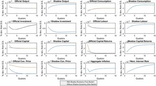
Figure 3. IRFs from effects of capital income tax shock.

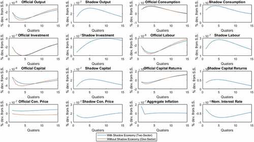
Figure 4. IRFs from effects of labour income tax shock.

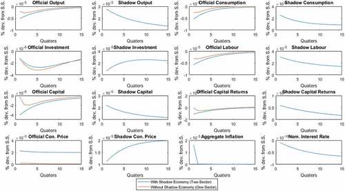
Figure 2 shows a response to a positive government spending shock and the model without a shadow economy indicated that employment, capital demand and product wage increase which increases official output. Similar results were obtained in the model with the shadow sector, with the main quantitative difference being the fall in official sector product wage. This shock comes in with two effects; demand for labour in the official sector leading to a rise in official labour employment and a negative wealth effect which reduces the consumption of official sector goods. With the rise in labour demand, employment increases and the real wage rate fall as a result of a fall in relative goods prices (see studies by Albonico et al. (2016) and Takyi and Leon-Gonzalez (2020a, 2020b) for similar findings). The reduction in the price of official sector goods leads to the reallocation of factors towards the official sector. This reallocation causes the shadow sector employment as a share of total employment to fall. On the response of labour employment and real wages, see, Pappa et al. (2015) for similar analysis on four Eurozone Takyi and Leon-Gonzalez (2020a, 2020b) for SSA countries.

Moreover, the persistent rise in nominal interest rate contributes to the fall in private consumption in both models. This is mainly caused by the negative wealth effects which arise from the increase in consumers’ anticipation of higher taxes in the future due to government spending hikes. This is consistent with Hayat and Qadeer (2016) for Asian countries; and Asif Khan and Khan (2011) for the Pakistani economy. On the other hand, the government spending shocks decrease the shadow sector variables including output, consumption, labour employment and capital demand which indicate a dampened effect of the shock on the informal sector. These results are expected since most of the government spending is geared toward the official sector.

Figure 3 presents the impulse responses of labour income tax hikes to the economy. It is immediately observed that the shock has a contractionary effect in the one-sector model and the official sector of the disaggregated model thereby reducing total output, private consumption, investment, labour employment and physical capital demanded by firms. The one-sector model shows that higher taxes raise the real wage, marginal cost of production and subsequently inflation. The increase in the cost of production through real wage and capital reduces labour demanded by firms and subsequent employment in the official sector and the aggregate demand through a fall in the private consumption expenditure by households since they supply labour demand and private investment (see, Albonico et al., 2016). The two-sector model also presented the negative effects of the shock in the official sector. However, the presence of the shadow economy has a powerful amplifying effect on the shadow sector’s real output, private consumption, private investment and labour employment. The presence of the shadow economy has a reallocation effect of factors services toward the shadow sector as a result of the fall in relative factor input prices (real wages) thus resulting in increasing production in the shadow sector and thereby the demand for shadow goods and services.

The results of an increase in capital income tax are presented in Figure 4. Official sector inflation and the nominal interest rate falls inducing a decrease in real interest rate causing an outflow of capital from the official sector to the shadow sector. This in turn lowers the official sector labour employment thereby inducing an increase in the shadow sector capital demand and labour employment as a result of a fall in shadow wages. This means that factor inputs with higher taxes in the official sector would outflow to the unofficial sector making the other factor inputs scarce in the shadow economy and this attracts an inflow of the scarce inputs as well. In the case of capital tax shock, the adjustment of capital is sufficient to generate the equilibrium dynamics. Overall, tax hikes lead to factor reallocation into the shadow sector. Higher taxes in the official sector provide incentives for tax evasion among firms and individuals. Moreover, the fall in investment and capital stock in the formal sector lowers the productivity differentials between the two sectors hence agents reallocate to the shadow sector leading to an increase in shadow sector labour employment and capital demand. An empirical work by Takyi and Leon-Gonzalez (2020a, 2020b) share a similar view on this study.

Figures 5–7 present the fiscal gap variables for output under the three fiscal instruments considered. The blue bars represent the fiscal gap variable in the model without a shadow economy and the orange bars represent the fiscal gap variable in the model with a shadow economy. The results from Figure 5 show that fiscal feedback stabilizes the positive government spending shock effects by reducing the output and this result is further strengthened in the model with a shadow economy. This is why the fiscal gap variable is negative during the periods considered. It strengthens the argument that fiscal stabilizers moderate overheating economies in periods of booms without affecting the underlying soundness of budgetary positions as long as fluctuations remain balanced. On the other hand, during recessions like our case with income tax hikes, fiscal stabilizers are to support economic activities.

Figure 5. Fiscal stabilizers—Government spending feedback.

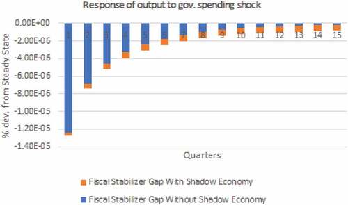
Figure 6. Fiscal stabilizers—Capital income tax feedback.

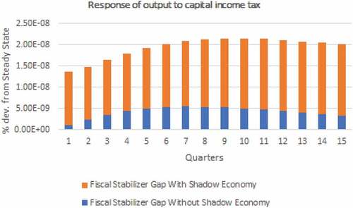
Figure 7. Fiscal stabilizers—Labour income tax feedback.

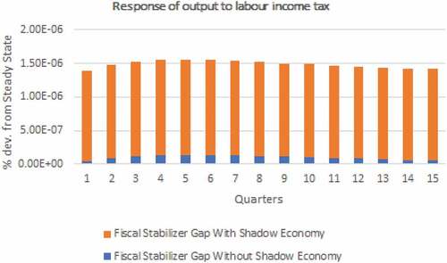
As shown in Figures 6 and 7, the fiscal feedbacks on taxes stabilize the economy by raising output in both models. The stabilization policies are strengthened with the introduction of the shadow economy. This indicated that fiscal feedback on government spending (income taxes) stabilized the economy by reducing (raising) output levels and these results even become stronger with the presence of a shadow economy. This robustness check further strengthens the important role of introducing the shadow sector into the model.

15. Conclusion and recommendations

The paper investigates the effects of fiscal policies in a New Keynesian DSGE framework with shadow economies. The study adds to the literature by extending the DSGE models by Smets and Wouters (2003); Albonico et al. (2016) and explicitly models fiscal policies to interact with monetary policy in the presence of informal economic activities in the SSA countries. The simulation involves exogenous processes that are asymmetric to the official sector consisting of government spending, labour and capital income tax shocks.

The message from the results is that shadow economic activities play a significant role in determining the behaviour of the real business cycle specifically the behaviour of the aggregate output. The results show that in economies with a large share of informal sectors like that of SSA countries, tax hikes lead to sizeable tax evasion and a boost in the activities of the informal sector making fiscal policies ineffective. The study also found that increase in public spending reduces shadow sector activities thereby increasing official sector GDP. This crowding-out effect contributes to obscuring the effectiveness of government spending and income tax on the aggregate GDP. The amplifying income tax effects occur simply because the effects of relative consumption and factor inputs prices create spill-over effects onto the shadow sector which determines the sectoral factor allocation in the model. The results from the fiscal feedback on government spending (income taxes) stabilized the economy by reducing (raising) output levels and these results even become stronger with the presence of a shadow economy. These results imply that, for effective implementation of government policies, policymakers must incorporate the activities of the informal sector into modelling and policymaking.

16. Further studies

The study can be expanded in the future to include an empirical econometric estimation for these selected countries. This estimation would then complement the theoretical model developed in this case. With data availability, the study could concentrate on country-specific to harness the full rigour of the model for policymaking. The theoretical model developed in the study can be expanded to include other macroeconomic and financial variables since they are connected to fiscal policy variables.

Acknowledgements

No fund or grant was received for this study.

Disclosure statement

No potential conflict of interest was reported by the author(s).

Additional information

Funding

The authors received no direct funding for this research.

Notes on contributors

Eric Amoo Bondzie

Eric Amoo Bondzie is currently a Lecturer at the Department of Economic Studies, University of Cape Coast – Ghana where he teaches both at the undergraduate and graduate levels. He holds a master’s degree in Economic Policy and Institutions from La Sapienza University of Rome and a PhD in Economics from the Catholic University of Milan all in Italy. His research areas are Macroeconomics, Monetary Economics, DSGE modelling and Time Series Econometrics.

Mark Kojo Armah

Mark Kojo Armah received his PhD in Economics at the University of Hull Business School’s Centre for Economic Policy in the U.K. He has consulting experiences with the AERC based in Nairobi, Kenya; and an active member of the American Economic Association. His research interest include exchange rate economics, energy economics, applied general equilibrium and poverty analysis in developing countries.

Notes

1. See contributions from (Albonico et al., 2016; Basile et al., 2016; Bhattarai & Trzeciakiewicz, 2017; Christiano et al., 2011; Coenen et al., 2012; Faia et al., 2013; Hemming et al., 2002).

2. Fiscal gap variable is defined as the difference between the variable value (output) in the case with fiscal stabilizers and the variable value in the case without fiscal stabilizers.

3. Smets and Wouters (2003, 2007) followed a partial indexation of prices.

4. Superscript i are ignored here.

5. The investment adjustment cost function is given by:

$S\left(\frac{i_t^i}{i_{t-1}^i}\right)=\frac{{\kappa }^I}{2}(\frac{i_t^i}{i_{t-1}^i}-1{)}^2$

In the steady state, $S\left(1\right)=S\prime \left(1\right)=0$, $S\left(1\right)>0\equiv \varpi$ with $\varpi$ being the adjustment cost parameter.

6. We assume a stochastic shock to the price of investment to affect only the official sector for tractability.

7. In the steady state, utilization cost function implies that: $u_s^i=1$ and $a\left(1\right)=0$.

8. In the official sector, consumption tax drives a wedge between final goods price set by firms and the corresponding consumption price.

9. See, Gali (2008). The labour market equilibrium requires that $w_t^i=mr{s}_t^i$, where $mr{s}_t=-U_{l,t}^i/U_{c,t}^i$ is the marginal rate of substitution between consumption and labour supplied in period $t+n$ for the households. This means that the official and shadow sector would pay the same consumption wage to workers.

10. A detailed derivations of all the first order conditions are available upon request.

11. In the steady state, we impose that $\frac{g_s}{y_s^o}=gs$ in order to obtain the public consumption-output ratio.

12. See, Coenen et al. (2012, 2013) for similar discussions. Here, the study does not necessarily consider feedback on debt and output but we assume the economy to react to fiscal shocks. Albonico et al. (2016) argued that a more restricted model without the feedbacks is better specified than models with fiscal reaction functions. Therefore, by considering fiscal shocks the model stability is obtained because the implicit lump-sum taxation ensures government solvency.

13. To the best of our knowledge, none of the empirical literature on SSA countries have estimated these feedback rule parameters. The study uses the parameter values from Coenen et al. (2012, 2013) and Corsetti et al. (2012) as a proxy for this work.

14. That is, deviation of inflation rate from the inflation target.

15. We note here that, the official sector resource constraint incorporates the government expenditure.

16. Through a straight forward manipulation using (9) and (10) we obtain steady state $SH$ as:

$SH=\frac{y_s^u}{y_s^o}=\frac{1-{\phi }_c}{{\phi }_c}(\frac{P_s^u}{P_s^o\left(1+{\tau }^c\right)}{)}^{-{ }_c}\frac{\left(1-i_s^o/y_s^o-g_s\right)}{\left(1-i_s^u/y_s^u\right)}$

17. The full set of the first order conditions, steady state derivations and log-linearized equations are available upon request.

References

- Acosta, P. A., Lartey, E. K., & Mandelman, F. S. (2009). Remittances and the Dutch disease. Journal of International Economics, 79(1), 102–21. https://doi.org/10.1016/j.jinteco.2009.06.007
- Albonico, A., Alessia, P., & Patrizio, T. (2016). In search of the euro area fiscal stance. Journal of Empirical Finance, 39, 254–264. https://doi.org/10.1016/j.jempfin.2016.06.007
- Amaral, P. S., & Quintin, E. (2006). A competitive model of the informal sector. Journal of Monetary Economics, 53(7), 1541–1553. https://doi.org/10.1016/j.jmoneco.2005.07.016
- Andolfatto, D. (1996). Business cycles and labor-market search. The American Economic Review, 86(1), 112–132. https://www.jstor.org/stable/2118258
- Annicchiarico, B., & Cesaroni, C. (2018). Tax reforms and the underground economy: A simulation-based analysis. International Tax and Public Finance, 25(2), 458–518. https://doi.org/10.1007/s10797-017-9450-7
- Aruoba, B. (2010). Informal sector, government policy and institutions. In 2010 meeting papers (Vol. 324).
- Asif Khan, S., & Khan, S. (2011). Optimal taxation, inflation and the formal and informal sectors (Tech. Rep.). State Bank of Pakistan, Research Department.
- Basile, R., Chiarini, B., De Luca, G., & Marzano, E. (2016). Fiscal multipliers and unreported production: Evidence for Italy. Empirical Economics, 51(3), 877–896. https://doi.org/10.1007/s00181-015-1026-8
- Batini, N., Levine, P., Lotti, E., & Yang, B. (2011). Informality, frictions and monetary policy. University of Surrey, School of Economics Discussion Papers, 711.
- Bhattarai, K., & Trzeciakiewicz, D. (2017). Macroeconomic impacts of fiscal policy shocks in the UK: A DSGE analysis. Economic Modelling, 61, 321–338. https://doi.org/10.1016/j.econmod.2016.10.012
- Chatterjee, S., & Turnovsky, S. J. (2018). Remittances and the informal economy. Journal of Development Economics, 133, 66–83. https://doi.org/10.1016/j.jdeveco.2018.02.002
- Christiano, L. J., Eichenbaum, M., & Rebelo, S. (2011). When is the government spending multiplier large? Journal of Political Economy, 119(1), 78–121. https://doi.org/10.1086/659312
- Coenen, G., Straub, R., & Trabandt, M. (2012). Fiscal policy and the great recession in the euro area. The American Economic Review, 102(3), 71–76. https://doi.org/10.1257/aer.102.3.71
- Coenen, G., Straub, R., & Trabandt, M. (2013). Gauging the effects of fiscal stimulus packages in the euro area. Journal of Economic Dynamics and Control, 37(2), 367–386. https://doi.org/10.1016/j.jedc.2012.09.006
- Cogan, J. F., Cwik, T., Taylor, J. B., & Wieland, V. (2010). New Keynesian versus old Keynesian government spending multipliers. Journal of Economic Dynamics and Control, 34(3), 281–295. https://doi.org/10.1016/j.jedc.2010.01.010
- Colciago, A., Ropele, T., Muscatelli, V. A., & Tirelli, P. (2008). The role of fiscal policy in a monetary union: Are national automatic stabilizers effective? Review of International Economics, 16(3), 591–610. https://doi.org/10.1111/j.1467-9396.2008.00747.x
- Colombo, E., Onnis, L., & Tirelli, P. (2016). Shadow economies at times of banking crises: Empirics and theory. Journal of Banking & Finance, 62, 180–190. https://doi.org/10.1016/j.jbankfin.2014.09.017
- Corsetti, G., Meier, A., & Muller, G. J. (2012). Fiscal stimulus with spending reversals. Review of Economics and Statistics, 94(4), 878–895. https://doi.org/10.1162/REST_a_00233
- Faia, E., Lechthaler, W., & Merkl, C. (2013). Fiscal stimulus and labor market policies in Europe. Journal of Economic Dynamics and Control, 37(3), 483–499. https://doi.org/10.1016/j.jedc.2012.09.004
- Fatas, A., & Mihov, I. (2001). The effects of fiscal policy on consumption and employment: Theory and evidence. In INSEAD mimeo, CEPR discussion paper.
- Gali, J. (2008). Introduction to monetary policy, inflation, and the business cycle: An introduction to the New Keynesian framework. Introductory Chapters.
- Gali, J., & Perotti, R. (2003). Fiscal policy and monetary integration in Europe. Economic Policy, 18(37), 533–572. https://doi.org/10.1111/1468-0327.00115_1
- Hayat, M. A., & Qadeer, H. (2016). Size and impact of fiscal multipliers: An analysis of selected south Asian countries. Pakistan Economic and Social Review, 54(2), 205. https://www.jstor.org/stable/26616707
- Hemming, R., Kell, M., & Mahfouz, S. (2002). The effectiveness of fiscal policy in stimulating economic activity: A review of the literature. IMF Working paper, 2002(Issue 208). https://doi.org/10.5089/9781451874716.001
- Junior, C. J. C., Garcia-Cintado, A. C., & Usabiaga, C. (2020). Fiscal adjustments and the shadow economy in an emerging market. Macroeconomic Dynamics, 1–35. https://doi.org/10.1017/S1365100519000828
- King, R. G., & Rebelo, S. T. (1999). Resuscitating real business cycles. Handbook of Macroeconomics, 1, 927–1007. https://doi.org/10.1016/S1574-0048(99)10022-3
- Koreshkova, T. A. (2006). A quantitative analysis of inflation as a tax on the underground economy. Journal of Monetary Economics, 53(4), 773–796. https://doi.org/10.1016/j.jmoneco.2005.02.009
- Krugman, P. (2012). Europe’s austerity madness. New York Times, 28, A35.
- Kumhof, M., & Laxton, D. (2007). A party without a hangover? On the effects of us government deficits. IMF working papers, 1–38.
- Larch, M., & Vandeweyer, M. (2013). Automatic fiscal stabilizers: What they are and what they do. Open Economies Review, 24(1), 147–163. https://doi.org/10.1007/s11079-012-9260-6
- Magazzino, C. (2022). Fiscal sustainability in the GCC countries. International Journal of Economic Policy Studies, 1–20. https://doi.org/10.1007/s42495-022-00082-9
- Magazzino, C., & Mutascu, M. I. (2022). The Italian fiscal sustainability in a long-run perspective. The Journal of Economic Asymmetries, 26, e00254. https://doi.org/10.1016/j.jeca.2022.e00254
- Makochekanwa, A. (2020). Informal economy in SSA: Characteristics, size and tax potential.
- Maloney, W. F. (1999). Does informality imply segmentation in urban labor markets? Evidence from sectoral transitions in Mexico. The World Bank Economic Review, 13(2), 275–302. https://doi.org/10.1093/wber/13.2.275
- Maloney, W. F. (2004). Informality revisited. World Development, 32(7), 1159–1178. https://doi.org/10.1016/j.worlddev.2004.01.008
- McKay, A., & Reis, R. (2016). The role of automatic stabilizers in the us business cycle. Econometrica, 84(1), 141–194. https://doi.org/10.3982/ECTA11574
- Medina, L., & Schneider, F. (2018). Shadow economies around the world: What did we learn over the last 20 years? International Monetary Fund.
- Melina, G., Yang, S.-C. S., & Zanna, L.-F. (2016). Debt sustainability, public investment, and natural resources in developing countries: The DIGNAR model. Economic Modelling, 52, 630–649. https://doi.org/10.1016/j.econmod.2015.10.007
- Merz, M. (1995). Search in the labor market and the real business cycle. Journal of Monetary Economics, 36(2), 269–300. https://doi.org/10.1016/0304-3932(95)01216-8
- Mountford, A., & Uhlig, H. (2009). What are the effects of fiscal policy shocks? Journal of Applied Econometrics, 24(6), 960–992. https://doi.org/10.1002/jae.1079
- Nguimkeu, P., & Okou, C. (2019). Informality. In Choi, J., Dutz, M., & Usman, Z. (Eds.), The future of work in Africa: Harnessing the potential of digital technologies for all (pp. 107–139). World Bank Group.
- Pappa, E. (2009). The effects of fiscal shocks on employment and the real wage. International Economic Review, 50(1), 217–244. https://doi.org/10.1111/j.14682354.2008.00528.x
- Pappa, E., Sajedi, R., & Vella, E. (2015). Fiscal consolidation with tax evasion and corruption. Journal of International Economics, 96, S56–S75. https://doi.org/10.1016/j.jinteco.2014.12.004
- Perotti, R., Reis, R., & Ramey, V. (2007). In search of the transmission mechanism of fiscal policy. NBER Macroeconomics Annual, 22, 169–249. https://doi.org/10.1086/ma.22.25554966
- Pratap, S., & Quintin, E. (2006). The informal sector in developing countries: Output, assets and employment (No. 2006/130). Research Paper, UNU-WIDER, United Nations University (UNU).
- Rotemberg, J. J. (1982). Monopolistic price adjustment and aggregate output. The Review of Economic Studies, 49(4), 517–531. https://doi.org/10.2307/2297284
- Rotemberg, J. J., & Woodford, M. (1992). Oligopolistic pricing and the effects of aggregate demand on economic activity. Journal of Political Economy, 100(6), 1153–1207. https://doi.org/10.1086/261857
- Schmitt-Grohe, S., & Uribe, M. (2004). Optimal fiscal and monetary policy under sticky prices. Journal of Economic Theory, 114(2), 198–230. https://doi.org/10.1016/S0022-0531(03)00111-X
- Schneider, F., Buehn, A., & Montenegro, C. E. (2010). New estimates for the shadow economies all over the world. International Economic Journal, 24(4), 443–461. https://doi.org/10.1080/10168737.2010.525974
- Singh, A., & Capt, J. (2002). Decent work and the informal economy: abstracts of working papers (Tech. Rep.). International Labour Organization.
- Smets, F., & Wouters, R. (2003). An estimated dynamic stochastic general equilibrium model of the euro area. Journal of the European Economic Association, 1(5), 1123–1175. https://doi.org/10.1162/154247603770383415
- Smets, F., & Wouters, R. (2007). Shocks and frictions in us business cycles: A Bayesian DSGE approach. The American Economic Review, 97(3), 586–606. https://doi.org/10.1257/aer.97.3.586
- Stiglitz, J. E., Fitoussi, J.-P., Bofinger, P., Esping-Andersen, G., Galbraith, J. K., & Grabel, I. (2014). A call for policy change in Europe. Challenge, 57(4), 5–17. https://doi.org/10.2753/0577-5132570401
- Takyi, P. O., & Leon-Gonzalez, R. (2020a). Macroeconomic impact of fiscal policy in Ghana: Analysis of an estimated DSGE model with financial exclusion. Economic Analysis and Policy, 67, 239–260. https://doi.org/10.1016/j.eap.2020.07.007
- Takyi, P. O., & Leon-Gonzalez, R. (2020b). Monetary policy and financial exclusion in an estimated DSGE model of sub-Saharan African economies. International Economic Journal, 34(2), 317–346. https://doi.org/10.1080/10168737.2020.1729835
- Taylor, J. B. (2009). The lack of an empirical rationale for a revival of discretionary fiscal policy. American Economic Review, 99(2), 550–555. https://doi.org/10.1257/aer.99.2.550