Fuzzy structural risk of default for banks in Southern Africa

Abstract

This paper proposes and examines a new structural risk of default model for banks in frictional and fuzzy financial markets. It is motivated by the need to fill the shortcomings of probability-based credit risk metric models that are characterised by unrealistic assumptions such as crisply precise and constant risk-free rates of return. The problem investigated here specifically proposes a new Kealhofer–Merton–Vasicek (KMV)-type model for estimation of the risk of default for banks extended for both market friction represented by transaction costs and uncertainty modelled by fuzziness. The novel risk of default model is then validated using cross-sectional financial data of eight commercial banks drawn from several emerging economies in Southern Africa. The results from the proposed model are fairly stable and consistent compared to those from hazard function and structural credit risk models currently used in the markets. The model is relevant in that it fairly captures practical conditions faced by banks that influence their risks of default in their quest to improve financial performance and shareholders’ wealth. The study recommends that banks in frictional and fuzzy financial markets, such as those in emerging economies, can adopt and implement the proposed risk of the default model.

Keywords:

• risk of default
• fuzzy financial markets
• risk metrics
• market friction
• fuzziness

JEL Classification:

• C13 and G24

Public interest statement

Risk of default measures the probability that a bank will not fulfil its principal and interest loan obligations due to its past commitments, current market, economic and liquidity circumstances. Investors must accurately measure the risk of default facing their financial investments in markets characterised by high transaction costs, also called market friction. The work proposes a model that incorporates vague concepts, such as high, medium and low volatility, covered in fuzzy logic or fuzziness, and market friction which characterise most emerging economies, in estimation of risks of default of banks. The results of the study are that banks’ risks of default are inversely related to their asset values, volatilities and returns on equity and directly correlated to market frictions and liabilities. Therefore, the study ends by recommending that banks must efficiently and effectively manage their investments in frictional and fuzzy financial markets to improve corporate performance and sustainability.

Abridged paper revision under summary of reviewer suggestions and comments

After going through suggestions and comments by Reviewers of our Risk of Default Paper, the following table summarises areas of concern that were noted for revision by the Reviewers:

Table

Suggestion/Comment by reviewer	Reviewer rating	Revision Made by author/s
Reviewer 2
Title, Abstract and Introduction	Outstanding
Methodology/Materials and Methods	Sound with minor or moderate revisions	The materials and methods used have been improved in terms of sequencing, language editing and overall presentation
Objectives/Hypothesis	Sound
Figures and Tables	Sound
Results/Data Analysis	Sound with minor or moderate revisionsProcedures and techniques used for data collection and analysis are partially adequate.	Sources of research data have been fairly articulated in line with expectations of the reviewer. The author/s took time to read through all paper results and data analysis to align them to the order of the objectives of the study. Presentation of paper results and analysis has been significantly revised to meet comments and suggestions by the reviewer.
Interpretation/Discussion	Sound with minor or moderate revisions Results must be supported by theory or empirical evidence and be well articulated	The interpretation and discussion improvements made to the paper are shown in BOLD in the relevant paper sections in much detail. The paper was then handed over to a language specialist after the above amendments to make sure grammatical issues are smoothened before sending it back to the Journal.
Conclusions	Sound
References	Sound
Compliance with Ethical Standards	Sound
Writing	Sound
Supplementary Information and Data	Sound
Reviewer 3
Title, Abstract and Introduction	Sound
Methodology/Materials and Methods	Sound
Objectives/Hypothesis	Sound
Figures and Tables	Sound
Results/Data Analysis	Sound
Interpretation/Discussion	Sound
Conclusions	Sound
References	Sound
Compliance with Ethical Standards	Sound
Writing	Sound with minor or moderate revisions	The paper writing style has been significantly improved. Paper has been proofread by a language editor to enable it meet the expected writing standard
Supplementary Information and Data	Sound

1. Introduction

The Merton (1974) structural probability of default (PD) model revolutionised research and practice in credit risk modelling in banking firms, and over the years, academic researchers and practitioners have extended Merton’s theory in various directions. For instance, structural credit risk models are based on the assumption that the non-stationary structure of the loan obligation leads to the termination of operations on a fixed date and default can only happen on a specified date. Geske and Delianedis (2003) extend the Merton asset valuation model (AVM) to the case of the valuation of tradable bonds with different terms to maturity. Their study concludes that it is incorrect to assume that the firm’s value of assets can be traded in financial markets. In reality, the value of the assets of a firm and its related parameters may not even be directly observed as articulated in most structural valuation models. This is one of the major drawbacks of structural credit risk models (CRMs) such as the Merton (1974) and Black and Scholes (1973) models that new models must seek to address.

Geske and Delianedis (2003) conclude that interest rates which are assumed to be fixed in the traditional PD model are random or stochastic. They go further to conclude that the yield spread curve in calibrated versions of the Merton model remains essentially zero for months, contrary to the observations made in real financial markets. On the one hand, structural models for the valuation of banks are based on the assumption that financial markets are perfect and frictionless. However, in practice, these markets are characterised by some degrees of friction and uncertainty such as fuzziness, vagueness, and ambiguity (Zadeh, 1965; Zimmermann, 1980). Therefore, the study proposes a KMV risk of default model extended for transaction costs for estimation of the risk of default in banks that operate in fuzzy financial markets.

2. Background to the study

Banks worldwide operate in financial markets characterised by some degrees of uncertainty, particularly in the forms of friction and fuzziness. Zimmermann (1980) and Zadeh (1965) demonstrate that most contemporary CRMs are suitable for the estimation of PDs of banks where transaction costs are negligible, minimal, or equal to zero. In reality, financial investors often subjectively express the uncertainty they face with some degree of implicit fuzziness also known as impreciseness (Zebda, 1989). For instance, investors may express market costs or returns as average, high or low, which terms are not explicit but implicit numbers. According to Zebda (1989), Zimmermann (1980), and Zadeh (1965), the investors’ use of operational language or semantics in market valuations is intrinsically imprecise contrary to some of the assumptions underlying most structural CRMs alluded to above.

However, the prerequisites of structural models such as Merton (1974) and Black and Scholes (1973) are that probability used in decision analysis is a ‘precise” number determined from repeated samples and relative frequency distributions (Kolmogorov, 1933). Kolmogorov’s classical probability theory differs significantly from fuzzy theory which is derived from the “degree of belief” set by financial experts and investors. Therefore, from the above observation, it becomes difficult to apply structural models to the valuations of risk metrics of banks under conditions of uncertainty in fuzzy decision-making processes (Bellman & Zadeh, 1970). In other words, we can conclude that investors use both probabilistic and fuzzy valuation tools to characterise the uncertainty that is inherent in financial market operations.

3. Problem statement

Contemporary literature has shown that traditional structural models such as the Merton (1974) are the cornerstones of all structural CRMs but are criticised for being constrained by their nature of not applying to frictional and fuzzy financial environments and underscoring the risk of default in good or boom economic times. Although some contemporary structural CRMs have been adjusted for fuzziness, especially in option pricing, none of them have been extended for market friction (Obeng et al., 2021; Tsunga et al., 2021). Hence, this research is motivated by the need to incorporate market friction and fuzziness in the valuation of the risk of default of banks to fairly reflect on practical conditions faced by investors. Banks in economies in Southern Africa are used because this is a region characterised by unique economic, business, and financial environments compared to other continents such as Europe and America.

4. Aim and objectives of the study

This study aims to improve the ability of structural models in the estimation of risk metrics concerning the modelling of the risk of default of banks. The objectives of the research study are to

Examine the impact of a KMV risk metrics model extended for both friction and fuzziness on the risks of default of banks in emerging financial markets.

Validate the proposed KMV risk of default model using financial data drawn from banks in emerging markets of countries in Southern Africa.

Compare the results estimated using the KMV risk of default model of banks with those generated from both hazard function and structural risk models.

5. Significance of the study

Although structural CRMs such as Merton (1974) and Black and Scholes (1973) are the benchmarks on which all bank and other firm valuations are based, they are usually criticised for being founded on unrealistic assumptions such as constant risk-free rates of return and frictionless markets. In practice, banks operate in frictional and fuzzy financial markets, contrary to the assumptions on which most structural CRMs are applied. Therefore, by extending contemporary structural models for market friction and fuzziness, banks can attain precision in the estimation of their risk metrics (Palma & Ochoa, 2013).

6. Research hypothesis

The study is carried out under the following hypothesis:

Null hypothesis (H0): Market friction and fuzziness have no effects on the DPs of banks in emerging economies.

7. Scope of the study

The study is carried out in Southern African countries mainly characterised by frictional and fuzzy financial markets. The study extends the existing structural models for market friction and fuzziness which are practical factors investors face in the valuation of banks and their risk metrics such as the risk of default (Obeng et al., 2021; Tsunga et al., 2021).

8. Organisation of the study

The paper is divided into five sections: the introduction above is Section 1 and Section 2 reviews literature on structural PD models, transaction costs, fuzzy set theory, and its applications. Section 3 proposes a new look KMV framework, Section 4 validates the model using financial data of eight banks from countries in Southern Africa and conclusions and recommendations of the study are then presented in Section 5 of the paper.

9. Literature review

This section examines the various theoretical frameworks underlying credit risk modelling with specific reference to the use of the hazard function and structural models in the estimation of the distances-to-default (DTDs) needed in the valuation of risk metrics of banks such as the risk of default. The evolution of CRMs starts by presenting the hazard function model by Cox (1972) before examining structural models such as Black and Scholes (1973) and Merton (1974) models and other relevant contemporary models on which the study leans.

9.1. Cox (1972)’s semi-parametric hazard function model and risk of default

The Cox proportional hazards model (Cox, 1972) is mainly a regression model that is commonly used in medical science research for modelling the association between patients’ survival data or times and one or more predictor or explanatory variables. This study starts by noting that there are two main classes of models that can be applied to credit risk modelling which are structural and reduced-form models. Structural models are used to calculate the probability of default for a form or bank based on its values of assets and liabilities. A firm defaults if its market value of assets falls below the debt obligations it has to pay or settle. A firm defaults if the market value of its assets is less than the debt it has to pay. The hazard rate function in the context of credit risk modelling is defined as the rate of default calculated at any time, assuming that the borrower has survived up to that point in time (Boland et al., 2016). The other name for the hazard rate is the marginal default probability (MDP) which is different from classical probability and survival analysis in credit risk modelling. Survival analysis has been introduced into credit scoring or rating in recent years. It is an area of statistics that deals with the analysis of lifetime data, where the variable of interest is the time of the event. The difference between hazard and survival functions is that a hazard function focuses on failing or an event occurring while a survival function focuses on an event not failing (Sawadogo, 2018). Therefore in some sense, a hazard function can be perceived as the converse side of the information provided by a survival function. The survival analysis model attempts to estimate the survival probability over the entire data set given. By comparison, risk represents probability while hazard represents settings, situations, or physical objects or phenomena.

Risk can be expressed in degrees, whereas hazards cannot be expressed in degrees. Hazard rates unlike classical probability theory can value values greater than 1 and technically cannot be a probability value. The hazard function can be interpreted as the conditional probability of the failure of a device at age X, given that it did not fail before the attainment of age X (Mendes, 2014). In other words, the interpretation and boundedness of a discrete hazard rate are different from those under the continuous probability case, such as the normal distributions. In reality, there are four main groups of work hazards faced, namely chemical, ergonomic, physical, and psychosocial, which can cause harm or adverse effects to humans in the workplace. Hazards must be identified first before a company undertakes a risk assessment, which implies that these two variables are different (Boland et al., 2016). In principle, a hazard is anything that could cause harm to a person or environment while the risk is a combination of two things which are the chance that the hazard will cause harm and the seriousness that the harm would cause. The hazard rate is sometimes referred to as the failure rate which is a rate that only applies to items or objects that cannot be repaired (Sawadogo, 2018). It is therefore fundamental to the design of safe systems in organisational applications and is often relied on in disciplines such as engineering, insurance, economics, finance, and banking and regulatory industries. The Cox (1972) model is presented in this section briefly to pave way for comparing results from its application in the study to those obtained from the traditional structural model and the proposed KMV risk of the default model.

9.2. Structural models for valuation of risk metrics of banking firms

Although the history of structural models backdates to before the Black and Scholes (1973) option pricing model (OPM), the models of management of credit portfolios are pioneered by Merton (1974). These models are then, developed further by Leland (1994), Leland and Toft (1996), Anderson and Sundaresan (1996), and Jarrow (2011). Although the Merton (1974) model is the benchmark on which all credit risk models are based, it is said to be limited in that it is only applicable when asset values and volatilities of firms are not directly observable. Secondary parameters of the Merton model such as $\mu \mathrm{a}\mathrm{n}\mathrm{d}\sigma$ (drift and asset volatility, respectively) are unknown and should be estimated from observed model parameters such as equity values and volatilities. Several estimation methods for the two parameters are applied in economics, business, banking, and finance, but not enough attention has been given to their theoretical and empirical shortcomings.

New models for the valuation of risk metrics of banks have been introduced in a somewhat unique liability structure in financial practice. Hence, emphasis needs to be laid on KMV methods and maximum-likelihood approaches to the valuation of risk metrics of banks. The KMV approach makes the Credit Analytics Services (CAS) offered by Moody’s KMV rigorous as detailed in the research by Crosbie and Bohn (2003). The two researchers start by describing KMV as a $\sigma$ restriction method without referring to Ronn and Verma’s (1986) model. However, they later take it as an iterative approach made up of the following steps:

Application of $\sigma$ to obtain a time series of implied asset values and hence compound asset returns continuously.

Use of time series of continuously compounded asset returns to obtain updated estimates for the unknowns, $\mu$, and $\sigma$.

Not going back to the initial stage with the updated $\sigma$ values unless convergence has been attained.

The KMV approach uses fixed maturity at 1 year and sets a default point to the sum of the short-term and half of the long-term debt obligations. According to Crosbie and Bohn (2003), the KMV suggests that firm defaults when its asset value falls somewhere between short-term default and the value of the total liabilities. The paper by these two uses KMV based on daily company market capitalisation together with quarterly updated debt levels for three banks to obtain the estimates needed. The study concludes that the KMV approach is an improvement in the distance-to-default (DTD) estimation models although it has its shortcomings. For instance, the KMV depends on the implied asset values and hence cannot be used to obtain unknown parameters in the capital structure of a firm. It also does not provide clear information on statistical estimations based on the Merton (1974) model. Bharath and Shumway (2008) argue that since Merton’s DTD model is not an econometric model, it is not clear how its parameters can be estimated using alternative techniques. Furthermore, it has been observed as unclear how standard errors for data forecasts can be calculated for the Merton DTD model whose application is premised on inaccurate or unrealistic assumptions.

Huang and Huang (2003) believe that there is no consensus from existing credit risk literature on how much observed corporate yield spreads can be explained by credit risk approaches. Their research concludes that using calibrated historical data, it is possible to obtain consistent estimates across credit spreads across all economic considerations within the credit risk structural frameworks. However, it has also been realised that credit risk explains just a small fraction of observed investment bond returns of all maturities together with a smaller fraction of short-term and higher fractions for junk bonds (Duan & Huang, 2012). Different structural DP models which generate high credit spreads are good in predicting fairly similar spreads under empirically reasonable choices of parameters, leading to the robustness of conclusions of the results of the paper by Huang and Huang (2003).

Bharath and Shumway (2008) examine the accounting and contributions of Merton’s (1974)’s DTD bond pricing model in comparison with the naive Merton model which cannot be applied in solving the implied probability of default (PD) model. Their research reveals that forecasting variables and naïve predictor models are better than hazard function models for in- and out-of-sample forecasts than both Merton DTD and reduced-form models that are based on sample inputs or variables. Fitted values drawn from expanded hazard models outperform Merton DTD-PD out of sample models. On the other hand, implied DTDs from credit default swaps (CDS) and corporate bond spreads are said to be weakly correlated with Merton DTD probabilities after adjusting for agency ratings and bond characteristics (Masatoshi & Hiroshi, 2009). The Merton DTD model is however criticised for not producing a sufficient statistical model for estimation of DPs of banks, making its functional form remain only useful for forecasting default events.

9.3. Estimation of DTDs for banking, financial and non-financial firms

Duan and Huang (2012) investigated several empirical applications to the estimation of DTD of banks. The DTD measures the extent to which a limited–liability corporation is away from a default event. Conceptually a firm’s asset values evolve according to a stochastic dynamic process where a debt (D) contract is honoured when the value of assets, A is greater than the promised payment to be settled in the future. Otherwise, if the above condition does not hold, a firm’s debt level, D and its debt holders can only recover a partial amount of what is left of the firm. When the current value of a company is much higher than its promised future obligations, the likelihood of the default event is small (Bharath & Shumway, 2008; Duan & Huang, 2012). This is because the firm has enough buffers to absorb losses in its asset values based on its corporate financial leverage (the debt-to-asset ratio) and the converse also holds. Since asset values move randomly due to external shocks, leverage ratios may not be good enough to fairly and adequately capture the notion of the DTD of a company. Some of the methods proposed in the literature used to estimate the unknown model parameters are:

The volatility restriction method by Jones, Mason and Rosenfeld (1984) and Rom and Verma (1996).

The transformation-data maximum likelihood technique by Duan (1994). The KMV iterative method was described in Crosbie and Bohn (2003) and the market value proxy method was used in Brockman and Turtle (2003) and Eom et al. (2004).

The model by Crosbie and Bohn (2003), for instance, uses financial firms to illustrate the shortcomings of the KMV-DP estimation model. The study concludes that financial firms have large proportions of liabilities for instance, policy obligations of insurance firms which cannot be accounted for by the KMV approach. The maximum-likelihood models by Duan (1994) are modified by Duan and Huang (2012) and Duan (1994) to deal with financial firms and are very appropriate and flexible techniques for use in the estimation of DTD. According to Duan and Huang (2012), the CRMs’ application of DTD makes it very unrealistic because its strict applications are at odds with empirical discount rates. Most financial academics argue that the DTD approach is highly informative about defaults but must be applied together with other variables to achieve good bank financial performance. According to Duan (1994), calibration through reduced-form models such as logit and logistic regression analyses should be a must take in all bank financial practices. However, it is ironic to argue that the DTD as a structural credit risk model (CRM) must be calibrated by a reduced-form model to give rise to good, precise, or accurate results. Based on the Merton (1974) model, it is assumed that firms are financed by equity, E with its value at the time, t, denoted by $S_t$, and one single pure discount bond (denoted by, $D_t$) with a maturity date, T and principal, F.

The asset value of the firm,$V_t$ is assumed to follow a geometric Brownian motion (GBM) given by the equation:

(1) $\mathrm{d}Vt={\mu }_A{V}_t\left(\mathrm{d}\mathrm{t}\right)+{\sigma }_A{V}_t{W}_t$(1)

where $V_t$ = A standard Brownian motion, ${\sigma }_A$= the volatility of assets, ${\mu }_A$ = the drift, and $d{W}_t$ = the Wiener process.

Due to banks’ operations under limited liability, the value of equity, $V_E$ at maturity is given by

(2) $\mathrm{S}\left(\mathrm{T}\right)=\mathrm{M}\mathrm{a}\mathrm{x}\left(V{A}_{,T}-\mathrm{F};0\right)$(2)

Hence, $V_E$ at t $\le T$ can be valued through the Black–Scholes OPM to become

(3) $\mathrm{S}\left(V{A}_t,{\sigma }_A\right)=V{A}_t\mathrm{N}\left(d_1\right)-e^{-r\left(T-t\right)}\cdot \mathrm{F}\times \mathrm{N}\left(d_1-{\sigma }_A\sqrt{\left(T-t\right)}\right)$(3)

where

(4) $d_1=\frac{ln(\frac{VA\left(t\right)}{F}+\left(r+\frac{{\sigma }^2}{2}\right)\left(T-t\right)}{{\sigma }_A\sqrt{\left(T-t\right)}}$(4)

S = the stock price,$V_A=\text{rm the{ } market{ } value{ } of{ } assets},{\sigma }_A=\text{rm the{ } asset{ } volatility},$ r = the instantaneous risk-free rate of return, F = the strike price of a call option, T = the term to maturity, t = time today, N($d_1$) and N($d_2$) = the cumulative probabilities of the Z-values, $d_1$, and $d_2$, respectively.

Due to the nature of diffusion models, $\mu$ cannot be estimated with high precision using frequency data over several years. This is true in financial econometrics because $\mu$ is accompanied by a time factor, $d_t$ whereas $\sigma$ is a time factor of $\sqrt{d_t}$, as implied in dWt. The frequency of data sampled is known for being less informative about $\mu$ than $\sigma$ because $d_t$ $<\sqrt{d_t}$ (Duan, 1994). When the value of $d_t$ is small, we can avoid the use of $\mu$ in DTD estimation particularly when this measure is used as an input in a reduced-form model that needs to be calibrated. Hence, the need to reduce sampling errors through the use of the alternative DTD formula given by

(5) $DT{D}_i^{\ast }=\frac{ln\left(\frac{Vt}{F}\right)}{\sigma \sqrt{T-t}}$(5)

In this respect, $DT{D}_i^{\ast }$ amounts to setting, $\mu$ = $\frac{{\sigma }^2}{2}$ in Equation 4(4) $d_1=\frac{ln(\frac{VA\left(t\right)}{F}+\left(r+\frac{{\sigma }^2}{2}\right)\left(T-t\right)}{{\sigma }_A\sqrt{\left(T-t\right)}}$(4) , making $DT{D}_i^{\ast }$ to be more stable than the traditional DTD.

9.4. Classical models for valuation of banks’ probabilities of default (PDs)

Nagel and Purnanandam (2020) point out that the distress faced by banks during the 2007–08 global financial crisis brought an urgent need for understanding and effective modelling of their PDs. Assessment of default risks for banks is fundamental to investors, risk managers, and regulators when it comes to the measurement of bank performances and failures. In all these applications, investors and risk analysts rely on structural models of default risk where equity (E) and debt (D) values are seen as contingent claims on the assets owned by the firms. For example, Merton’s (1974) standard approach or model assumes that the value of assets of a firm follows a log-normal process that is options embedded in the firm’s E and D values which can be valued using the Black and Scholes (1973) model.

Extensive financial literature employs the Merton (1974) model to price deposit insurance in particular (Rennacchi, 1988; Ronn & Verma, 1986, Marcus; Shaked, 1984). It is argued that Merton’s log-normally distributed asset values may provide some useful approximation for the asset value process of non-financial firms. However, this assumption is very problematic for banks that include debt claims such as mortgages whose upside payoffs are limited contrary to the requirements of the log-normal distribution which postulates that the upside is unlimited. The model by Nagel and Purnanandam (2020) uses capped upside of a bank’s assets. The study uses the log-normal distribution assumption on the assets of borrowers of a bank as collateral security.

The bank’s assets are modelled as a pool of zero-coupon bonds whose repayments depend on the value of the borrowers’ collateral assets at loan maturity as postulated in Vasicek (1991).

The model by Nagel and Purnanandam (2020) also stipulates that loans issued have variable maturities which means that every time a fraction of a loan portfolio matures, the bank issues repayment proceeds as a set of new loans at a fixed initial loan-to-value ratio. If a loan becomes delinquent, the pledged collateral is replenished to the extent that the initial loan-to-value ratio is then satisfied. Lastly according to Nagel and Purnanandam (2020) and Vasicek (1991), the bank’s assets, A, E and D, are assumed to be contingent claims on the borrowers’ collateral assets. According to the study, all loans issued have values of 1.60 and debt has a face value of 1.20. This implies that the maximum that the bank can recover in the event of default is the loan value (1.60). This is capped when the borrower’s assets value falls below 1.60 because the assets of the bank are sensitive to the borrower’s asset values as demonstrated below.

Figure 1. Assets of a bank sensitised by those of the borrower.

Source: Authors.

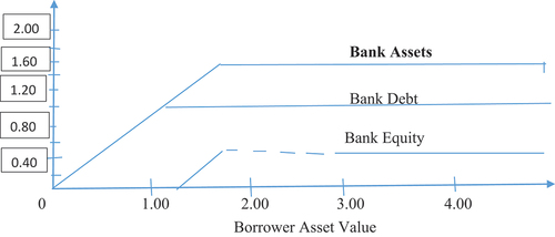
Figure 1 shows that the value of the bank’s assets cannot have a log-normal distribution. This is because its borrowers maintain the upside of their assets’ values above the face value of the loans. The bank’s equity payoffs do not resemble a call option written on an asset with an unlimited upside, but rather a mezzanine claim comprising two kinks. These kinks have implications for the risk dynamics of the equity of a bank and the estimation of its risk of default (Nagel & Purnanandam, 2020). Under a capped upside, the volatility of a bank’s assets will be very low in good economic times such as booms when asset values are high. At maturity, asset values will end up running parallel to the right where banks’ equity payoffs are insensitive to variabilities in the borrower’s asset values. The Merton’s (1974) standard model in which the equity of a firm is assumed to be a call option on an asset with significant variability will miss all these non-linear risk dynamics. In times of high asset values, banks may show many asset volatilities away from default, a conclusion that could be very misleading. This is because it ignores the fact that bank asset volatilities may dramatically rise if the values of its assets fall. Merton’s standard model could end up making misleading predictions about the riskiness of the values of the bank’s assets, debt, and equity.

9.5. Option pricing models (OPMs), uncertainty and estimation of PDs of banks

Nowadays many phenomena in economics, business, banking, and finance are uncertain or fuzzy but are treated as if they were crisp or precise in all decisions of banking firms and similar financial institutions. However in practice, prediction of both business and consumer bankruptcy is imprecise and ambiguous (Korol, 2008). The financial performance and PD modelling of banks are affected by both internal and external factors that cannot be precisely and unambiguously defined. The mere allegation that a company is at risk of bankruptcy must not be considered imprecise. In economic reality, there are more firms or persons than can be considered 100% bankrupt. It is difficult to accurately determine the degree of bankruptcy of a bank using structural statistical methods such as multivariate discriminant analysis (MDA). Fuzziness is defined by Zimmermann (2001) and Zadeh (1980) as a market condition in which returns to financial market investments are not precisely defined as expressed in probability theory but in linguistic terms such as high, average, or low. With the use of fuzzy logic and vague and ambiguous concepts, banks’ risk metrics can be defined as “high“ or ”low” risk of bankruptcy (Korol, 2008; Zimmermann, 1980).

The precisions on which structural CRMs are based are influenced by deduction and thinking processes that use a non-binary logic with fuzziness. The Merton (1974) and Black and Scholes (1973) models, for instance, do not put fuzziness into consideration when dealing with all the aforementioned financial problems. Banks’ CRMs such as the one by Appadoo and Thavaneswaran (2013) are structural valuation models that involve uncertainty that arises from lack of knowledge, inherent vagueness, or imprecision. Of late there has been growing interest by researchers to use fuzzy numbers to deal with vagueness and imprecision facing investors in financial markets (Appadoo, 2006). More researchers such as Yu et al. (2011) and Cherubini (1997) deal with randomness in European OPMs. These models are extended to the case for pricing corporate debt contracts and provide a fuzzified version of the Black and Scholes (1973) model using a variety of input variables. Results realised from the application of their models have improved estimation precision, robustness, and consistency in the pricing of options in fuzzy financial markets.

Ghaziri et al. (2000) use an artificial intelligence approach to the pricing of options using neural networks and fuzzy logic and compare their results to those obtained using the Black–Scholes stock indices. The study concludes that the Black–Scholes OPM is an approximation model which leads to a considerable number of errors. Trenev (2001) came up with a refined option pricing formula and discovers that because of the fluctuating nature of financial markets over time, some of the parameters of the Black–Scholes model may not be expected in the precise or exact sense. Thavaneswaran et al. (2007) apply fuzziness to the Black–Scholes OPM and conclude that it is far from being practical. Although the Black–Scholes OPM is flexible and can be applied to the valuation of banks and their risk metrics, it is criticised for being premised on precise variables such as frictionless markets.

Chang and Huang (2020) apply a fuzzy credit risk assessment model in banks and conclude that financial institutions need to regularly update their assessment models to maintain correct assessment results. They note that every update involves a lot of numerical experiments using multiple systems or software packages for the evaluation of the effects of different sampling techniques and classifiers to construct suitable models for the updated data sets. Chang and Huang (2020) used the latest web-based technology to develop a fuzzy decision support system (DSS) that used logistic regression as the classifier combined with various sampling methods and model threshold settings to come up with a model fitting process that is more structured and efficient. Therefore by fuzzifying the independent variables of the proposed DP model, the study intends to make the new model efficient and accurate. Zhao and Dian (2017) argue that fuzzy credit risk models must be premised on stable conditions and effectiveness to reduce the conservativeness of the imperfect circumstances found in the real markets. On the other hand, Sakai and Kubo (2011) argue that institutional investors attain estimation rigour by assessing credit risk by using a combination of quantitative information, for example, OPMs and qualitative assessments.

Although structural OPMs can be easily constructed, they are mainly suitable for the assessment of long-term credit risk where the probability of bankruptcy varies directly with the timing of the assessment. Sakai and Kubo (2011) propose a new set of assessment models for long-run credit risk that does not use stock prices and incorporates business cycles. Values estimated from these models are effectively usable in the calculation of risk spreads such as DTDs although rating biases may exist in the credit risk assessment of the markets. Schultz et al. (2017) employ Merton’s PD as a continuous ex-ante measure of the likelihood of a firm’s failure to perform on a loan obligation. They apply a dynamic generalised methods of moments (GMM) to characterise the link between corporate governance and the chance of default by a financial institution.

By using the GMM technique, the research overcomes the limitations of discrete proxies used in previous similar studies. Initial test results demonstrate that there is a significant relationship between a bank’s PD and corporate governance measured in terms of executive remuneration, board, and ownership structures. However, when endogenous factors are accounted for in the above model, relationship ceases to exist. Malyaretz et al. (2018) substantiate the need to incorporate efficiency indicators of bank activity as fuzzy quantities to fairly demonstrate the actual conditions faced by institutional investors in emerging markets. They propose a fuzzy multivariate regulatory analysis model for the assessment of the competitiveness of Ukrainian commercial banks. The results of their research show that there is the expediency of the application of the model to determination of the competitiveness of banks drawn into the study.

According to Lee et al. (2005), the Black–Scholes option model developed in 1973 has always been considered the cornerstone of all OPMs. However, its practical applications have always been constrained by its nature of not being suitable for fuzzy financial market environments. Hence, since the planning and decision-making processes of investors in the area of option-pricing are always with a degree of uncertainty, it is pertinent that new structural models for estimation of risk metrics be adjusted to improve their precision and accuracy (Zadeh, 1965; Zimmermann, 1980). In reality, option pricing methods depend on a person’s deduction and thinking process which employs a non-binary logic with fuzziness which is not considered by classical probabilistic models such as the Black–Scholes model. Lee et al. (2005) adopt a fuzzy decision tree and Bayes’ rule as a base for measuring fuzziness in options’ analysis and pricing. Their study also employs a fuzzy decision space comprising four dimensions, namely fuzzy state, sample information, action, and evaluation function to describe investors’ decisions to derive a fuzzy Black–Scholes OPM under a fuzzy financial environment. The results of the research by Lee et al. (2005) show that the market risk-free rate of return, stock price, and call prices in the money (ITM) and at the money (ATM) are over-estimated while that of the out of the money (OTM) option is under-estimated. It is the flexibility demonstrated by the Merton (1974) model that exploits the flexibility of the Black–Scholes OPM to come up with an asset valuation model (AVM) on which all contemporary structural credit risk models are premised.

9.6. Contemporary credit risk models for estimation of PDs of banks

According to Engelmann and Rauhmeier (2011), the use of internal rating-based approaches (IRBA) of the new Basel Capital Accords is critical as it allows banks to use their rating models for the estimation of PDs provided their systems meet the set minimum requirements. Statistical theory provides a variety of methods for building and assessment of credit rating models. These methods include linear regression modelling, time-discrete techniques, binary response analysis, hazard models, and non-parametric models such as neural networks and decision trees such as the Bayes’ theorem. The benefits and drawbacks of the above models are interpreted in light of the minimum requirements of the IRBA. Engelmann and Rauhmeier (2011) discover that although there are difficulties such as data collection processes and procedures, model building, and time and effort took in model validation, IRBA is efficient and maintains its predictive power in the estimation of the risk of default of a bank. In other words, contemporary IRBA must maintain their linearity assumption to be always reliable and valid in their application to the valuation of credit exposures of banks.

Kholat and Gondzarova (2015) compare characteristics and mutual relationships among contemporary CRMs based on the importance of credit risk issues in the global economy and business sector operations. Their study examines Credit-Metrics and Credit Risk + models whose parameters are based on differences in computational procedures and model techniques used in the quantification of input parameters. They use variables such as risk definitions and sources, characteristics and data requirements, credit events, returns, and numerical model designs across various CRMs to come up with their models. They realise that effective models to do with credit risk need to be based on default-mode and marking-to-market (MTM) models, a result consistent with that by Gisho and Khestick (2013). Default mode is a technique used in the prediction of bank losses caused by default events arising from failure and non-failure model variables. This is the case for Credit-Risk+ and Moody’s KMV) models which are improvements to the structural risk metric models by Merton (1974) which is drawn from the Black and Scholes (1973) OPM.

MTM models on the other hand contain the Credit-Metrics approach and focus on the market values of loans. These models use rating systems (rating migration) to determine changes in the loan quality of a potential borrower. It is noted that default mode models are only measured by changes in the debtors’ assessments which emanate from their failure to honour their loan obligations. The models compare the possible paths of loan default rates under both Credit-Metrics and Credit-Risk+ models (Musankova & Koisisova, 2014b). Credit-Metrics and KMV models are based on the traditional Merton (1974) model and hence banks’ assets and their volatilities are central data variables that are needed in the estimation of the risk of default of a bank. On the other hand, the major variables under Credit-Risk+ models are default risk levels and asset volatilities. The paper by Musankova and Koisisova (2014b) discovers that KMV data inputs are a time series of asset values comprising risk liabilities, stock prices, and asset correlations. The characteristics of credit events can also be used to compare CRMs, for example, the creditworthiness of bondholders. In this respect, the KMV determines a credit event of a bank as a change in the distance-to-default (DTD) which leads to changes in the expected default frequency (EDF; Gavlakova & Kliestik, 2014). The Credit-Metrics model on the other hand characterises credit events as states in which there are migrations of default events from one grade to another. Empirical evidence suggests that EDF values respond to changes in the credit quality of borrowers faster than changes in their rating classifications.

Therefore, we can conclude that credit events are more prevalent in the KMV than in Credit-Metrics models and hence the need to adopt the former for its ability to estimate prevalent credit events. Under Credit-Risk+, credit events are based on default-state because they are unique. Default mode models and changes in default rates may imply decreases in the credit quality of a borrower. The estimation of the DP of a bank and the distribution function of the default probability of $\sigma$ of a credit event in the Credit-Metrics approach is represented by the default probability modelled based on its annual historical data (Kliestik et al., 2015). Under the KMV approach, the expected frequency of failure changes in response to variabilities in market values of assets and their standard deviations. On the other hand, their paper determines that under Credit-Risk+, default probability is represented by a measure of the risk of default (Gavlakova & Kliestik, 2014). The recovery rates under default events are exogenous parameters for each sub-portfolio of loans used in the Credit-Risk+ approach. However, under the Credit-Metrics approach, these recovery rates are captured as random variables with beta distributions and modelled using the Monte Carlo Simulation approach. The simple KMV considers recovery rates to be constant model parameters, while the KMV model assumes that these rates follow a beta data distribution. Hence, it is based on gaps in contemporary structural credit risk models presented above that this study proposes a KMV-DP estimation model extended for market friction to make it reflective of the practical conditions faced by investors and banks in fuzzy financial markets.

9.7. Market friction and variables of the proposed KMV default probability model

This subsection intends to provide the link between the literature detailed above and the proposed KMV risk of default model’s variables which are market values and volatilities of banks and return on equity (ROE) and market friction.

9.7.1. The concepts of market efficiency and friction

Calin (2016) defines market efficiency as the extent to which the price of an asset or stock fully reflects all information available and hence this makes financial markets frictionless. However, economists disagree on how efficient markets are attained and frictionless. Followers of the efficient market hypothesis by Fama (1952) hold that markets efficiently deal with all information on a given security and reflect it in the stock price immediately. Therefore, technical and fundamental analysis methods of stock pricing and/or any speculative investing based on these methods are useless. A frictionless market can be defined as a theoretical trading environment where all costs and constraints associated with transactions are non-existent (Downey, 2019). However, the primary observation of behavioral economics, for instance, holds that investors make decisions on imprecise impressions and beliefs, rather than rational analysis. This, therefore, renders financial markets somewhat inefficient to the extent that they are affected by the decisions of investors and people in general.

argue that markets are frictionless when efficiency in capital markets requires that capital flows are sufficient to eliminate arbitrage anomalies. The authors examine the relationship between capital flows to a quantitative (quant) strategy. This is a strategy based on capital market anomalies and the subsequent performance of the financial institutions after the implementation of this strategy. When capital flows are high, holders of quantitative funds can implement arbitrage strategies more effectively, leading to lower profitability of market anomalies in the future, and the converse is also true. This means that the degree of cross-sectional equity market efficiency varies across time factors with the availability of arbitrage capital. Frictionless markets are used in theory to support investment research or financial trading concepts. In speculative investments, many financial performance returns will assume frictionless financial market costs.

Investors must view both friction and frictionless analyses for a realistic understanding of a security’s return on the market of operation. Pricing models such as Black and Scholes (1973) and other methodologies also make frictionless market assumptions which are important to consider since actual transaction costs will be associated with real-world financial applications. In economic theory, a frictionless financial market is defined as a market without transaction costs to be faced by investors (Downey, 2019). Friction on the other hand is a type of market incompleteness. Every complete market is frictionless, but the converse does not hold. In a frictionless market, the solvency cone is the half-space normal to the unique price vector. The Black–Scholes OPM is based on the assumption of a frictionless market that is a market where investors incur no transaction costs in all their banking and investment endeavours (Durbin, 2002).

De-Young (2007) defines market frictions as all transaction costs, taxes and regulations, asset indivisibility, nontraded assets, and agency and information problems that negatively impact the performance of banks and other players. These costs are not provided for in contemporary CRMs making all asset, equity, and risk metric estimates from banks’ financial data to be inaccurate and not true reflections of their actual financial performances. These costs facing banks are made very high when additional hazards such as regulatory and supervision and corporate governance and ethical challenges are factored into the estimation of risk metrics. Fuchs and Uy (2010) note that a lack of technology and innovations bring huge barriers to further outreach and development, including high transaction costs and lack of access to long-term sources of finance.

Although structural models assume that markets are frictionless, in reality, financial markets are characterised by friction as evidenced by changing asset standard deviations and returns to investments. It is observed that costs of making financial transactions are very huge and not constant as purported by popular CRMs by Merton (1974), Black and Scholes (1973), and De-Young (2007) define market friction as anything that interferes with investors’ trading and can exist even in efficient markets. They go further to argue that financial market frictions generate business opportunities and costs to investors and change over time.

9.7.2. Relationship among variables of the proposed KMV-DP model

Traditional and asset value volatility movements must play an indispensable role in the determination of the likelihood of default events (Mason & Rosenfeld, 1984). This is because the same level of the buffer may not be sufficient to withstand potential losses when the value of a firm’s assets is highly volatile. Under good economic times, a good DTD value must be a leverage ratio adjusted for the trend and a standard deviation of the value of a firm’s assets. Duan and Huang (2012) introduced the Merton model to define the DTD of banks above. The DTD is an appropriate concept used in the estimation of default risk. However, it is challenged because it is computed only when we know the market values of assets and parameters governing both trend and asset volatilities. The asset values and volatilities are not observable when used under the standard Merton (1974) model. In the absence of a time series of observed asset values, it is complex to estimate model parameters that define both trends and movements in standard deviations of assets.

Risk of default or DP is the likelihood that a bank will fail to perform on its interest and principal obligations when they fall due. Default risk occurs when the market values of banks’ assets lose value in the financial markets (Sakai & Kubo, 2011). In other words, when assets default, a bank must reduce the values of such assets on its books, following its laid down accounting standards and rules, and decrease its capital values and earnings. DP is a very important risk metric that must be efficiently or effectively estimated to improve precision and robustness in the assessment of bank financial performance (Engelmann & Rauhmeier, 2011). Effective DP estimation can also enable banks to come up with critical policies and strategies for reducing the quantity of non-performing loans (NPLs) and financial performance. In the study, the risk of default is the dependent variable, and market friction (cost of equity), bank liabilities, asset values, and their volatilities, time to maturity, and return to equity are the independent variables. The discussion below details all the independent variables of the proposed model, and how they are estimated from the raw data before they are fuzzified using contemporary models presented in Sections 3 and 4.

10. Market values of banks and their volatilities

Using Ito’s Lemma, we can demonstrate that the values of equity and assets of a bank and their volatilities can be connected through the general formula:

(6) ${\sigma }_E=\frac{V_A}{V_E}\times \frac{d{V}_E}{d{V}_A}{\sigma }_A$(6)

To be able to solve for the unobservable variables of the equation, namely $V_A$ and ${\sigma }_A,$ we should be able to solve a system of non-linear equations. The famous Merton (1974) PD model as applied by Garcia et al. (2021) gives rise to two simultaneous linear equations (7(7) $V_E=V_A\times N\left(d_1\right)-e^{-rT}X\times N\left(d_2\right)$(7) and 8(8) ${\sigma }_A=\frac{V_A}{V_E}\cdot \times N\left(d_1\right){\sigma }_A$(8) ) with two unknowns which are $V_A$ and ${\sigma }_A$:

(7) $V_E=V_A\times N\left(d_1\right)-e^{-rT}X\times N\left(d_2\right)$(7)

The volatilities of equity and assets of a banking firm are connected through the equation:

(8) ${\sigma }_A=\frac{V_A}{V_E}\cdot \times N\left(d_1\right){\sigma }_A$(8)

Asset volatilities represent how large a company’s assets swing around the mean market price that is it is a statistical measure of the returns to a bank. The values of a bank’s assets and their volatilities are unknowns to be estimated from the financial fundamentals of the bank under structural models 7 and 8.

11. Estimation of the liabilities of a bank

The basic accounting equation used in the estimation of a bank’s liabilities is Assets (A) = Liabilities (L) + Owner’s equity (S), such that Liabilities, L = A-S. In the model, a bank’s Total assets = Non-current assets+ Current assets, Liabilities = Long-term Liabilities+ Current liabilities, and Owner’s equity = Number of shares issued $\times \mathrm{M}\mathrm{a}\mathrm{r}\mathrm{k}\mathrm{e}\mathrm{p}\mathrm{r}\mathrm{i}\mathrm{c}\mathrm{e}\mathrm{p}\mathrm{e}\mathrm{r}\mathrm{s}\mathrm{h}\mathrm{a}\mathrm{r}\mathrm{e}.$ The current liabilities of a bank include all current payments on long-term loans such as mortgages and deposits by its clients.

12. Return on equity and its estimation

Return on equity (ROE) is defined as the company’s average residual or net income per share in the issue. According to Burns et al. (2008), the ROE is a better way or measure of bank profitability than the risk-free rate of rate which is just a nominal and not effective measure of bank performance. Most structural models of default risk are pinned on the risk-free rate of return, which is far from reflecting fairly the actual performance of a bank. Hence, the study employed the banks’ ROEs as these fairly represented a true reflection of their actual position from all their trading and investment activities over a given time frame. ROEs are strong proxies for the risk-free rates of return because they are unique and directly related to the individual bank’s issued shares and market financial performances. The banks’ ROEs are calculated using the traditional formula,

(9) $\mathrm{R}\mathrm{O}\mathrm{E}=\frac{NetIncome\left(EarningsAfterIn\mathrm{t}erestandTax\right)}{TotalMarketoftheFirm{ }^{\mathrm{\prime }}sOrdinaryEquity}.\hspace{0.17em}$(9)

Banks’ ROEs like all other risks of default model variables are converted into fuzzy values because they are also influenced by experts’ perceptions.

13. Estimation of the cost of equity

One of the major contributors to the risk of default in banks is the cost of equity which is not factored into most contemporary structural models (Besley et al., 2020). Cost of equity can be defined as the return that a company needs for a project or investment or equity investment or pays out to ordinary shareholders as dividends. According to Zabai (2019) in conjunction with Madan and Unal (1996), banks must manage their default risks through efficient, effective and prudential management of their costs of equity. The study, therefore, incorporates market friction in the form of the cost of equity, in the proposed KMV risk of default model to represent costs incurred by banks in constituting their capital bases. We used Myron Gordon’s constant growth model to estimate the bank’s cost of capital or the required rate of return (RRR). The traditional RRR or cost of equity is calculated using Gordon’s constant growth model or formula,

(10) $\mathrm{R}\mathrm{R}\mathrm{R}=\frac{D_0\left(1+g\right)}{P_0}+g$(10)

where ${\mathrm{D}}_0=\mathrm{T}\mathrm{h}\mathrm{e}\mathrm{d}\mathrm{i}\mathrm{v}\mathrm{i}\mathrm{d}\mathrm{e}\mathrm{n}\mathrm{d}\mathrm{p}\mathrm{e}\mathrm{r}\mathrm{s}\mathrm{h}\mathrm{a}\mathrm{r}\mathrm{e}\mathrm{p}\mathrm{a}\mathrm{i}\mathrm{d}\mathrm{t}\mathrm{o}\mathrm{d}\mathrm{a}\mathrm{y},$ $P_0=$ The market price per share today, and g = The constant growth rate in earnings and dividends.

14. Research methodology

We proceed by first illustrating the fuzzy logic, concepts, and approach to the estimation of risk metrics of banks before presenting the proposed KMV risk of default model, assumptions, sources of data and input variables, and their justification.

14.1. Fuzzy approach to estimation of the risk of default of a bank

This section commences by presenting the basic fuzzy concepts of fuzzy sets and systems before proposing the model to be used in calculating the risk of default of banks.

14.1.1. Fuzzy concepts and their definitions

The following are the basic definitions and properties of fuzzy set theory, systems, and numbers with their relevant operations.

Definition 3.1 A fuzzy set, A in X $\in$ R (real numbers), is a set of ordered pairs A =$\left\{\left(\mathrm{x};\mu \left(\mathrm{x}\right):\mathrm{x}\in \mathrm{X}\right)\right.$ where $\mu \left(\mathrm{x}\right)$ is the membership function, grade of membership, degree of compatibility, or truth of x $\in \mathrm{X}\mathrm{w}\mathrm{h}\mathrm{i}\mathrm{c}\mathrm{h}\mathrm{m}\mathrm{a}\mathrm{p}\mathrm{s}\mathrm{x}\in \mathrm{X}\mathrm{o}\mathrm{n}\mathrm{t}\mathrm{o}\mathrm{t}\mathrm{h}\mathrm{e}\mathrm{r}\mathrm{e}\mathrm{a}\mathrm{l}\mathrm{i}\mathrm{n}\mathrm{t}\mathrm{e}\mathrm{r}\mathrm{v}\mathrm{a}\mathrm{l}\left[0;1\right]$ (Chen & Pham, 2001).

Definition 3.2 A fuzzy set A in $R^n$ is said to be a convex fuzzy set if its $\gamma -[\mathrm{l}evelsetA\left(\gamma \right)$ are (crisp) convex sets for all $\gamma \in \left[0;1\right],{\mu }_A\left(\lambda x_1+\lambda x_2\right)\ge Min\left({\mu }_A\left(x_1\right);{\mu }_A\left(x_2\right)\right)\left(\mathrm{A}\mathrm{p}\mathrm{p}\mathrm{a}\mathrm{d}\mathrm{o}\mathrm{o}\mathrm{a}\mathrm{n}\mathrm{d}\mathrm{T}\mathrm{h}\mathrm{a}\mathrm{v}\mathrm{a}\mathrm{n}\mathrm{s}\mathrm{w}\mathrm{a}\mathrm{r}\mathrm{a}\mathrm{n},2013\right).$

Definition 3.3 A fuzzy number, u =$\left\{a^{-}\right.$, a,$a^{+})$ is specified by its core a $\in Randamembershipfunctio\mathrm{n},\mu :R\to \left[0;1\right]$ with support in [$a^{-};a^{+}$] defined as:

(11) $\mu \left(x\right)=\left\{\begin{array}{c}L\left(x\right)if{a}^{-}\le x\le a\\ R\left(x\right)ifa\le x\le a^{+}\\ 0Otherwise,\end{array}\right.\mathrm{f}\mathrm{o}\mathrm{r}\mathrm{x}\in R,$(11)

where L(x) is an increasing function with L($a^{-}$) =0, L(a) =1 and R (x) is a decreasing function with R (a) =1, R ($a^{+})=0.$ Functions L(.) and R (.) are the left and right shape functions of u, and they are assumed to be differentiated (Chen and Pham, 2001).

Definition 3.4 For values of $\propto \in [0,1,the\propto -cut$ s are defined to be the compact intervals ${\left[u\right]}_{\propto }$=$\{)$ $\left\{x|\mu \left(x\right)\ge \propto \right\}$, which are “nested” closed intervals (Wang Y, Elhag T MS, 2006).

14.1.2. Fuzzy approach systems and their applications

Fuzzy approach systems have not only been used in a variety of practical problems but also in regulatory risk and credit analysis, as well as for evaluation of bankruptcy and default prediction. The fuzzy approach combines easy designs based on both experts’ opinions and data history in the estimation of the risk of default of a bank, leaving out market friction. Fuzzy logic arises as a good tool for emulating expert rules since they do not require too much effort to modelling risk metrics as other traditional methods do (Chen & Pham, 2001). A fuzzy system can emulate rules of the common type: IF (Conditions) THEN $\left\{\mathrm{C}\mathrm{o}\mathrm{n}\mathrm{s}\mathrm{e}\mathrm{q}\mathrm{u}\mathrm{e}\mathrm{n}\mathrm{c}\mathrm{e}\mathrm{s}\right\}$, where conditions and consequences are fuzzy propositions built by linguistic expressions or semantics:

1. x is Low

2. y is Not High

3. x is Low AND y is High

4. x is Low OR y is High.

Propositions 1 and 2 (expressions) define immediate propositions, while propositions 3 and 4 define combined propositions (Soares et al., 2013). Since these terms operate over fuzzy variables, we need to define them in linguistic terms or fuzzy sets, as covered or defined in Section 3.0. Fuzzy expressions to do with semantics such as NOT, OR, and AND, which are combined to form relations, R are detailed in Section 4.

14.2. Proposed KMV-risk of default model for commercial banks

The study proposes a risk of default model that incorporates the variables of the distance-to-capital (DTC) model but is based on the DTD valuation model. The DTC takes precedence over the DTD because the latter model does not involve complexities that are related to the firm’s numerical fundamentals. According to Larsen and Mange (2008), a firm’s DTC, at the time, t can be computed from the general formula:

(12) $DTC\left(t\right)=\frac{log(\frac{V_A\left(t\right)}{\rho X\left(t\right)}+\left(r-\frac{{\sigma }_A^2}{2}\right)\left(T-t\right)}{{\sigma }_A\sqrt{\left(T-t\right)}}$(12)

where $V_A$ (t) = The market value of the bank’s assets at the time, t, X(t) = The market value of debt, r = The risk-free rate of return, T = The term to maturity of assets or debt, ${\sigma }_A=\mathrm{T}\mathrm{h}\mathrm{e}\mathrm{a}\mathrm{s}\mathrm{s}\mathrm{e}\mathrm{t}\mathrm{v}\mathrm{o}\mathrm{l}\mathrm{a}\mathrm{t}\mathrm{i}\mathrm{l}\mathrm{i}\mathrm{t}\mathrm{y},$ $\rho =\frac{1}{1-PCAR}$, where PCAR = The capital requirements of a bank according to the Capital I Accord set at 8% of the risk-weighted assets of a bank. It should however be understood that for the calculation of the DTD we take $\rho =1.0$ 0 and PCAR = 0. The conversion of the Merton–KMV–DTD model to a risk of default model calls for deducting transaction costs from the risk-free rate of return obtained in the economy. Therefore, the proposed KMV model for the valuation of the risk of default of banks drawn from the above equations is given by:

(13) $\mathrm{D}\mathrm{P}=\frac{N\left[ln\left(\frac{V_A\left(t\right)}{X\left(t\right)}\right)+\left(\mu -k_e+\frac{{\sigma }_A^2}{2}\right)T\right]}{{\sigma }_A\sqrt{T}};$(13)

where $\mathrm{l}\mathrm{n}=\mathrm{T}\mathrm{h}\mathrm{e}\mathrm{n}\mathrm{a}\mathrm{t}\mathrm{u}\mathrm{r}\mathrm{a}\mathrm{l}\mathrm{l}\mathrm{o}\mathrm{g}\mathrm{a}\mathrm{r}\mathrm{i}\mathrm{t}\mathrm{h}\mathrm{m},\mu =\mathrm{T}\mathrm{h}\mathrm{e}\mathrm{r}\mathrm{e}\mathrm{t}\mathrm{u}\mathrm{r}\mathrm{n}\mathrm{o}\mathrm{n}\mathrm{e}\mathrm{q}\mathrm{u}\mathrm{i}\mathrm{t}\mathrm{y},\mathrm{a}\mathrm{n}\mathrm{d}{\mathrm{k}}_{\mathrm{e}}=\mathrm{T}\mathrm{h}\mathrm{e}\mathrm{c}\mathrm{o}\mathrm{s}\mathrm{t}\mathrm{o}\mathrm{f}\mathrm{c}\mathrm{a}\mathrm{p}\mathrm{i}\mathrm{t}\mathrm{a}\mathrm{l}.$ The study uses the return on equity (ROE) instead of the risk-free rate of return because it is more characteristic of the fair returns to banks than the latter. Following the Merton (1974) model, we can show that the risk of the default probability of a bank at the time, T evaluated at the time, t is given by

(14) $\mathrm{D}\mathrm{P}=\mathrm{N}\left(-\mathrm{D}\mathrm{T}\mathrm{D}\right)$(14)

where DTD at the time t is given by

(15) $DT{D}_t=\frac{ln(\frac{V_A\left(t\right)}{X_t}+\left(\mu -\frac{{\sigma }_A^2}{2}\right)\left(T-t\right)}{{\sigma }_A\sqrt{\left(T-t\right)}}$(15)

where $\mu$ = the expected market rate of return.

Since the Standard Normal Distribution (0;1) function is universal, the side factor that determines the DP of a bank is the DTD. The DTD is simply the logarithm of the leverage ratio shifted by the expected return (u-$\frac{{\sigma }^2}{2}$) (T-t) and scaled by the volatility-time term, $\sigma \sqrt{(T-t}$). If we have two firms with identical leverage ratios and asset $\sigma$ deviations but the asset value of one firm is expected to increase at a faster rate than that of the other, it means that results will depend on the sign attached to the numerator (Dua et al., 2012). When the numerator is positive the assets of the firm will cover default and lower, ${\sigma }_A$, making the firm less likely to default and vice versa. The implication is that when economic agents are risk-neutral, the expected investment return will be $R_f$ that is $\mu$ should be replaced by $R_f$. In theory, DP is not physically experienced but DTD is, hence the need for suitable estimates for both expected return and $\sigma$.

Two models adopted for comparison with the proposed KMV model are the traditional structural PD and hazard function models whose formulae are outlined below:

The structural probability of default (PD) model for comparison with the proposed model (equation 13(13) $\mathrm{D}\mathrm{P}=\frac{N\left[ln\left(\frac{V_A\left(t\right)}{X\left(t\right)}\right)+\left(\mu -k_e+\frac{{\sigma }_A^2}{2}\right)T\right]}{{\sigma }_A\sqrt{T}};$(13) ) is given by the formula:

(16) $\mathrm{P}\mathrm{D}=\frac{N\left[ln\left(\frac{V_A\left(t\right)}{X\left(t\right)}\right)+\left(\mu +\frac{{\sigma }_A^2}{2}\right)T\right]}{{\sigma }_A\sqrt{T}}$(16)

The Cox (1972) proportional hazard function model discussed in Section 2.1 of the literature is based on two major assumptions: (1) survival data curves for different strata should have hazard functions that are proportional over the time frame, t and (2) the relationship between the logarithmic hazard and each covariate are linearly related, which can be verified with residual data plots. It has been shown that when the hazard ratio is >1.00, the treatment group would have a shorter survival span than the control-referenced group (Sawadogo, 2018). On the other hand, if this ratio is <1.00, it implies that the group of interest is less likely to have a shorter time to the event than the reference group. The ratio is however criticised for not being able to quantify the magnitude of the difference between the two groups. While the logistic regression model tests whether a risk factor affects the odds of a disease or not, the Cox (1972) proportional hazards model tests whether a risk factor affects the age of onset of the disease in humans. Any hazard ratio above 1.00 would generally mean that the treatment group healed faster or had a slower time to an event. A hazard ratio of 1.00 means that both groups (control and treatment) would be experiencing an equal number of events at any given point in time (Mendes, 2014).

According to Sawadogo (2018), the Cox (1972) semi-parametric model is a regression approach for human survival data that provides an estimate of the hazard ratio and its corresponding confidence interval, which is an area of interest to credit risk modelling under frictional and fuzzy financial markets. The study uses the Cox (1972) proportional regression model which fits data with a constant covariate, xx that is data that do not vary over time to a hazard function of the general form given by

(17) $h\left(t|x\right)=\mathrm{h}\left(\mathrm{t}|\mathrm{x}\right)=h_0\left(\mathrm{t}\right)\mathrm{e}\mathrm{x}\mathrm{p}\left[{\beta }_1\mathrm{x}\right]\mathrm{h}\left(\mathrm{t}/\mathrm{x}\right)=h_0\left(\mathrm{t}\right)\mathrm{e}\mathrm{x}\mathrm{p}[{\beta }_1\mathrm{x}]$(17)

where we can estimate the unknown value of β1 and h0(t) is the baseline hazard, which is a non-parametric and unspecified value that depends on the variable tt and not on xx. Therefore for particular xx values, we will be able to estimate the survival function if we have an estimate of the baseline survival function,$S_0$ (t) $S_0$^(t; Boland et al., 2016). The estimated survival function for an individual human with covariate value xk turns out to be given by

(18) $\mathrm{S}\left(\mathrm{t}/\mathrm{x}\mathrm{k}\right)=[S_0\left(\mathrm{t}\right)]\mathrm{e}\mathrm{x}\mathrm{p}({\beta }_1\mathrm{x}\mathrm{k})S_0\left(\mathrm{t}/\mathrm{x}\mathrm{k}\right)=[S_0\left(\mathrm{t}\right)]\mathrm{e}\mathrm{x}\mathrm{p}({\beta }_1\mathrm{x}\mathrm{k})$(18)

The study adopts the form of the hazard model above to determine the hazard rates of banks when it comes to their failure to meet their debt obligations. Cox’s (1972) model is used in the study mainly for comparing results with those drawn from the structural and proposed KMV risk of the default model. It should however be noted that there are usually magnified differences between hazard and credit risk model ratios because risk ratios do not care about the timing of the event but are only concerned about the occurrence of the event by the end of the day.

14.2.1. Sources of data

The study used audited and published financial data of eight banks conveniently drawn from six Southern African countries. The countries from which the banks are drawn are South Africa, Namibia, Botswana, Malawi, Tanzania, and Zambia. The audited financial statements of the banks cover the period 2008–2020 and are from the World Development Index (WDI, 2020). This is a credible source of data and researchers can easily download data directly from the website for research purposes. Although the available financial data are drawn from various economies of Southern Africa, the research concentrates on financial data of banks listed on Stock Exchanges of the same countries. Panel data are popular for their ability to reduce the co-linearity among explanatory variables, and hence improve the efficiency of econometric estimates. The study employs unbalanced panel data that have been checked and screened for apparent coding errors and missing variables. It is the interest of the research to conveniently draw various countries from the region in the quest to compare and contrast the performances of banks in large and small countries such as South Africa and Mauritius, respectively.

14.2.2. Input variables for the proposed model and their justification

The data variables for the estimation of the risk of default for a bank are market values of its assets (A) and debt (D), asset volatility, the return on equity ($\mu$) $,andcostofcapital\left(k_e\right).$ Extension to existing CRMs such as KMV DTD-PD for market friction enables investors to improve the accurate estimation of their banks’ PDs. According to KMV-DTD model, the equity of a firm is perceived as a call option on its underlying assets because at the maturity of debt, bondholders receive their debts and equity holders realize the rest. The model operates only if we are given observable equity and unobserved asset values and their corresponding volatilities. Based on the Black–Scholes OPM, where the value of assets is represented by the price of a call option (C) and the value of equity by the value of the stock (S), debt (D) is taken as the strike price (K).

14.2.3. Assumptions of the KMV risk of default model

The assumptions on which the KMV model is founded are two, that is

Debt is homogeneous with time to maturity, T;

The Capital Structure of a firm is given by the general equation:

(19) $V_A\left(\mathrm{t}\right)=\mathrm{D}\left(\mathrm{t}\right)+V_E\left(\mathrm{t}\right)$(19)

where $V_A$ (t) = the value of assets, D(t) = the value of debt and $V_E$ (t) = the value of equity.

The markets are perfect and ignore coupons and dividends and there are no penalties incurred by investors for short selling; and

Dynamism of a bank’s assets is that they follow a geometric Brownian motion as alluded to earlier on under equation 1(1) $\mathrm{d}Vt={\mu }_A{V}_t\left(\mathrm{d}\mathrm{t}\right)+{\sigma }_A{V}_t{W}_t$(1) .

Under the Black–Scholes OPM, the market price of a European call option is given by

(20) $\mathrm{C}\left(\mathrm{t}\right)=\mathrm{S}\left(\mathrm{t}\right)\mathrm{N}(d_1)-e^{-r\left(T-t\right)}.\mathrm{K}\mathrm{N}(d_2)$(20)

where S(t) = the stock price, r = the risk-free rate, K = the strike price of a call option, T = term to maturity of the bank’s assets and liabilities, t = time today, N($d_1$), and N($d_2$) = the cumulative probabilities of the Z-values,$d_1$, and $d_2$, respectively.

Using Ito’s Lemma we have demonstrated that the values of equity and assets of a bank and their volatilities can be connected through the general formula above (see equation 6)(6) ${\sigma }_E=\frac{V_A}{V_E}\times \frac{d{V}_E}{d{V}_A}{\sigma }_A$(6) . To solve equation 6(6) ${\sigma }_E=\frac{V_A}{V_E}\times \frac{d{V}_E}{d{V}_A}{\sigma }_A$(6) for the unobservable variables of the equation, namely $V_A$ and ${\sigma }_A,$ we should be able to solve a system of non-linear equations given by

(21) $\left\{\begin{array}{c}{f}_1\left(V_E;{\sigma }_E\right)=V_A\left(t\right).N\left(d_1\right)-e^{-\left(r-k_e\right)\left(T-t\right)}.DN\left(d_2\right);V_E\left(t\right)=0\\ f_2\left(V_E;{\sigma }_E\right)=\frac{V_A}{V_E}.\frac{d{V}_E}{d{V}_A}N\left(d_1\right){\sigma }_A;{\sigma }_E=0\end{array}\right.$(21)

The solutions to the above system of equation (13)(13) $\mathrm{D}\mathrm{P}=\frac{N\left[ln\left(\frac{V_A\left(t\right)}{X\left(t\right)}\right)+\left(\mu -k_e+\frac{{\sigma }_A^2}{2}\right)T\right]}{{\sigma }_A\sqrt{T}};$(13) are unique as

(22) $\frac{d{f}_1}{d{V}_E}=\mathrm{N}(d_1);$(22)

which is analogically due to changes in the Black–Scholes model and $f_1$ is an increasing function of the value of assets of a bank,$V_A\hspace{0.17em}thatis{f}_1\left(V_A\right)$ has a unique solution. On the other hand, $f_2\left({\sigma }_E\right)$ has a unique solution as well.

14.3. The structure of a fuzzy system

According to Soares et al. (2013), a fuzzy system is usually characterized by the following components:

Input variables (made up of their respective fuzzy data sets)

Output variables (these are the diagnostic values)

Rule base (this determines the output for each combination of input values)

Inference machine (which applies fuzzy operations to transform crisp variables into fuzzy variables)

Fuzzy sets (these are linguistic terms for each input variable drawn into the model)

Crisp values (these are numerical values taken from the real financial world)

The four model variables namely expected return on equity ($\mu ),/break\mathrm{c}\mathrm{o}\mathrm{s}\mathrm{t}\mathrm{o}\mathrm{f}\mathrm{e}\mathrm{q}\mathrm{u}\mathrm{i}\mathrm{t}\mathrm{y}({\mathrm{k}}_{\mathrm{e}}),\mathrm{a}\mathrm{s}\mathrm{s}\mathrm{e}\mathrm{t}\mathrm{v}\mathrm{a}\mathrm{l}\mathrm{u}\mathrm{e}\mathrm{s},\mathrm{a}\mathrm{n}\mathrm{d}\mathrm{v}\mathrm{o}\mathrm{l}\mathrm{a}\mathrm{t}\mathrm{i}\mathrm{l}\mathrm{i}\mathrm{t}\mathrm{i}\mathrm{e}\mathrm{s}$ are fuzzified through the architecture of fuzzy systems given below, developed by Ross et al. (2010).

14.4. Concepts used in the architecture of fuzzy systems

The principal components of fuzzy logic control systems are the fuzzifier, rule base, and evaluation, aggregation of the rule outputs, and de-fuzzification as detailed below.

15. Fuzzification

This is the process of transforming real-world crisp quantities into fuzzy quantities or variables (Ross et al., 2010). This can be realised by identifying the various precise and deterministic quantities as totally non-deterministic and very uncertain in practice. These variables’ uncertainty could have emerged as a result of imprecision and vagueness which may then lead to the representation of the input variables by a membership function as they can be fuzzy. For example, if we argue that the return to equity of a bank is 25% per annum, an investor could convert this crisp input into a linguistic variable such as moderate, high, or low return (Ross et al., 2010). The study transforms the four input variables, ROE, cost of equity, asset values, and volatilities into fuzzy parameters for use in the estimation of the risks of default of banks. The fuzzifier translates these crisp variables into fuzzy inputs which are then directed into the intelligence engine for further transformation. The intelligence engine is responsible for converting the input variables into fuzzy outputs. All the fuzzy outputs obtained are then directed into the de-fuzzifier where they are finally turned into crisp outputs.

16. Fuzzy operations, rules, base, and evaluation

This is the application of fuzzy operations, Minimum and Maximum in input variables according to the available rules to determine if they should be inclusive (AND) or exclusive (OR). The fuzzy rules comprise input and output variables that assume values from their term sets, with meanings associated with each linguistic concept (Soares et al., 2013). Crisp or exact model inputs are fed into the fuzzifier to transform them into fuzzy variables under a clearly defined rule base. The rule base is characterised by all the rules and membership functions that regulate decision-making processes in fuzzy logic systems. The base also contains the “If-Then” conditions which are used for conditional programming and controlling the whole fuzzy logic system. Rules evaluation is a technique that is used to assess the criteria and return model values based on a dynamic configuration process (Ross et al., 2010). The evaluation system gives users the possibility to configure model inputs for application scoring, approving flows, credit insurance, or bureaus.

17. Aggregation of the rule outputs

The aggregation of the rule outputs is the process by which the fuzzy sets representing the outputs of each rule are combined into composite fuzzy sets. It is a process that only occurs once for each output variable and happens before the final de-fuzzification process is undertaken. The output of the aggregation process is converted into one fuzzy set for each given output variable.

18. De-fuzzification

This is the opposite of the process of converting the crisp results into fuzzy variables. The mapping done here is the conversion of the fuzzy results into crisp variables. This process is very capable of generating a non-fuzzy control action which illustrates the possible distribution of an inferred fuzzy control action or process (Ross et al., 2010). The de-fuzzification process can also be considered to be the rounding-off process, where a fuzzy set having a group of membership values on the unit interval is transformed into a single scalar quantity.

19. Validation of the KMV-Risk of dealt model, findings, and discussions

The validation of the proposed risk of the default model follows several steps as detailed below.

19.1. The fuzzy extension principle

It has been observed that most structural stochastic models are solved using classical and fuzzy set theories but are not extended for market friction which is a huge transaction cost to investors, especially in emerging financial markets. In the process of managing functions of real variables, the use of the fuzzy extension framework should result in the correct application of the extension principle by Talamanca, Guerra, and Stefanini (2011). We start by assuming that we are given an exact relationship function of the general form,

(23) $y=F(x_1;x_n;------;x_n)$(23)

of n real variables given by $(x_1;x_n;------;x_n)$. The above multiple linear relationship function’s fuzzy extension can be obtained to evaluate the effects of both transaction costs and uncertainty on the variable, $x_j$, modelled by the corresponding number, $u_j$ for each level $,\alpha$ in the interval [$u_{j,\alpha }^{-}$; $u_{j,\alpha }^{+}$,], given the possible values $of{x}_j$. Suppose we are also given another variable, $v=f(u_1;u_n;------------;u_n)$;which denotes the fuzzy extension of a continuous function, f. The continuous function, f is characterised by n variables for each level of $\alpha$, resulting in the interval [$v_{\alpha }^{-}$; $u_{\alpha }^{+}$], which represents the propagation of uncertainty from all variables, $x_j$ to the variable, $\gamma$ (Ross et al., 2010).

It should be noted that if the uncertainty on the original variables of a model is denoted by, $\gamma ,$ which is also modelled by linear numbers, the $\gamma$-variable will still be a fuzzy number, starting from a single value (at $\alpha$ =1.00) to the most uncertain interval level (at level, $\alpha$=0.00), but it loses its linearity property in the process of such transformation (Soares et al., 2013). This also follows that the parametric representation of the variable is also necessary when input variables are triangular fuzzy numbers to apply the extension principle and represent the non-linear output fuzzy numbers (Talamanca, Guerra, and Stefanini, 2012). To obtain the fuzzy extension of fuzziness to normal semi-continuous fuzzy intervals, we have to compute the $\alpha$–cuts [$v_{\alpha }^{-}$; $u_{\alpha }^{+}$] of v, defined as the images of $\alpha$-cuts of $(u_1;u_n;-------;u_n)$; that are then obtained by solving the following constrained optimisation problems for $\alpha \in$ [0;1]:

(24) $(EP)\alpha =\left\{\begin{array}{c}(v_{\alpha }^{-}=min\{f\left(x_1;x_2;--;x_n\right)xk\in [u{k}_{\alpha }^{-};u{k}_{\alpha }^{+}\left],k=1;2;---;n\right]\\ (v_{\alpha }^{+}=max\{f\left(x_1;x_2;--;x_n\right)xk\in [u{k}_{\alpha }^{-};u{k}_{\alpha }^{+}\left],k=1;2;---;n\right]\end{array}\right.$(24)

Source: Talamanca, Guerra and Stefanini (2012).

Only in simple cases can the optimising problems above be solved analytically. In general, the solution of such a system of equations is complex and computationally expensive to determine for each $\alpha \in$ [0;1]. Hence, we require global solutions to the two non-linear problems for all model variables. Therefore, Ross et al. (2010) present the above architecture of fuzzy systems which we used in translating input variables of the KMV risk of the default model into fuzzified parameters.

19.2. Settings and implementation of the fuzzy system

The fuzzy system elaborated above is implemented using Mamdami’s (1975) system as the central inference machine. This is because Mamdami’s system is very simple for use in processing rules and values of model variables. The system is set up as tabulated below for fuzzification and de-fuzzification of model variables:

19.3. Fuzzy logic and DP modelling in banks

Fuzzy logic has been defined as a computing technique based on the degree of truth. It may also be taken to be a method of reasoning that resembles human logic or reasoning in financial investment decisions. The approach of fuzzy logic imitates the way of decision-making in humans that involves all intermediate possibilities between two digital values, which are “Yes and No” (Chen & Pham, 2001). Therefore, fuzzy logic operates on the levels of possibilities that are associated with the input variables to attain a definite model output. Fuzzy logic is thus a basic control mechanism that depends on the degrees of the state of the input variable/s. It is the state of the input used in modelling that determines the nature of the output to be realised. A study by Sabounchi et al. (2011) uses fuzzy logic that incorporates linguistic variables in the valuation of a default event. The study concludes that the use of the max-min operator system diversifies inconsistencies among fuzzy rules and defuzzified model variables behaved reasonably for defuzzified default risk estimation methods. In other words, a fuzzy logic system works on the principle of assigning a particular output depending on the probability of the state of the input variable to be used. There are many reasons given for the application of fuzzy logic in banking and finance such as

It is relatively simple to create and deploy since it’s fully based on human experts’ opinions and evaluations.

It is used in fields of study involving decision-making processes that require some sort of human judgment.

Human mind abstracts real-world variables in an imprecise manner to constitute semantic networks.

These semantic variables or networks define relations that can be expressed in linguistic terms just as experts do in various disciplines (Soares et al., 2013).

Hence, any business activity that requires expert opinions or judgments can be modelled through fuzzy logic rules without the need for an existing theoretical model to base on. By taking into account all the above sets of fuzzy sets, numbers, and logic or literature into consideration, we designed a model for predicting the risk of default of banks that could be accurate, robust, and practical. The methodology used in this design is the same as that which was developed and employed by (Pereira et al., 2012). The research methodology we use comprises the following procedure or variables running from stages A to C:

According to literature, the default event is influenced by many borrower internal and external conditions most of which could be unknown to the loan provider unless they are declared. However, simple models of DP can yield good results using statistical measures or techniques (Ross et al., 2010). To make the system more applicable, we took all the crisp variables of the model and fuzzified them before the validation of the proposed KMV-DP model.

19.4. Results from validation of the KMV-risk of default model

The study proposes a new look KMV model for estimation of the DP of a bank in emerging financial markets. It investigates the effects of asset values, liabilities, returns on equity and cost of equity or friction on the DPs of banks in fuzzy financial markets. The model is validated using financial data drawn from banks in emerging markets of countries in Southern Africa. It also aims to compare the results estimated using the KMV model with those generated from other approaches such as hazard function and structural risk models. The research employs a STATA Package to come up with three sets of results for all eight banks based on structural, fuzzy KMV, and hazard function models for comparison purposes. Table 1 represents the architecture of fuzzy system by Ross et al. 2010 which was adopted for fuzzification of model variables. Table 2 on the other hand demonstrates hoe model variables where fuzzified and defuzzified. On the other hand Table 3 presents the three stages of the study procedure or variables.Table 4 summarises the risks of default results from the structural and KMV models (in Scientific form, A $\times {10}^{-3})\mathrm{a}\mathrm{n}\mathrm{d}\mathrm{h}\mathrm{a}\mathrm{z}\mathrm{a}\mathrm{r}\mathrm{d}\mathrm{r}\mathrm{a}\mathrm{t}\mathrm{i}\mathrm{o}\mathrm{s}$ (as decimals).

Table 1. The architecture of fuzzy systems by Ross et al. (2010)

Structure of Fuzzy Systems (Source: Ross et al., 2010).

Table 2. The process of fuzzification and de-fuzzification of model variables

Variable/Approach	The system applied
Input fuzzy sets	Gaussian
Output fuzzy sets	Triangle
Implication method	AND/OR
Aggregation method	Product (AND)
De-fuzzification method	Centre of gravity

Table 3. The three stages of the study procedure or variables

A. Definitions of variables	B. Definitions of rules	C. Definitions of inferential machine settings
Sets of definitions	Operational research	Aggregations
Membership functions	Database formations	De-fuzzification

Source: Authors.

The results of the study show that all independent variables namely market values and their volatilities, liabilities, return on equity and cost of equity influence the risk of default of a bank. The study also postulates that asset values and volatilities and return on equity are inversely related to the risk of default of the bank (Appendix IV). The results concur with those of the standard structural model research study by Nagel and Purnanandam (2019) that risk of default and equity values of banks are more sensitive to negative shocks than to asset values and volatilities. The inverse relationship between the risk of default of a bank and stock returns signifies the presence of inefficiencies in the financial markets which motivated the undertaking of this study.

The above research result is contrary to the finding of a similar research study by Chava and Purnanandam (2010) that realises a positive cross-sectional relationship between stock returns and the risk of default of a bank or similar financial firm. Therefore, financial investors expect higher returns as compensation for bearing investment risks, and thus accords with the direct and fundamental principle of high risk, high return and low risk, low return. However, it is not very clear why some rational investors do not exploit such arbitrage opportunities to improve their financial performance in these markets. The study also acknowledges that the liabilities of a bank are directly related to the risk of default on its obligations and this is in line with results of a similar research study by Zabai (2019). In other words, a bank has a higher default risk when it has a poor credit risk rating and limited cash flow base.

The main independent variable drawn into the model is the cost of capital (a form of market friction), which is a function of the market’s risk-free rate of return plus a premium or compensation for the risk associated with the bank’s investment. The study further discovers that the cost of capital like the bank’s liabilities has a positive relationship with its risk of default level (Appendix I). This result concurs with findings of a related research by Gleibner (2019) which argues that financial markets are not perfect and are always frictional. Therefore, this study postulates that the cost of capital has a direct impact on risk of default of a bank and hence the need for it to be included in estimation of risk metrics. Uncertainty in the form of fuzziness is provided for in the variables of the proposed KMV-risk of the default model. It is observed that uncertainty is an economically important risk factor in the estimation of DPs of banks. This is because it captures variables such as corporate governance, economic booms, and recessions and expert judgments such as bullish and bearish market conditions (Switz et al., 2018). The study reveals that fuzziness is an uncertainty that increases the risk of default in banks as it lowers their overall financial performance and profitability.

According to Zhang et al. (2021), uncertainty is an economically significant risk with a direct bearing on banks’ risks in that it increases the risk of default of borrowers. Effective governance of such uncertainty can alter the risk-increasing and profit-decreasing effects of bank performance. The results of the study also demonstrate that good and strong corporate governance and ethics mechanisms play a key role in weakening the hazardous consequences of economic uncertainty on banks and the promotion of sustainable growth and development of the banking sector. This research observation supports the findings of a related study by Switz et al. (2018) that ownership structure has a significant impact on default risk of financial firms and none on non-financial firms. The study further notes that the bigger the independent board of directors of financial institutions, the higher the risk of default and the lower the risks facing non-financial institutions. This research study also finds that there is a direct linkage between the bank and market sizes and the risk of default faced. According to a study by Laeven et al. (2014), unconditional risk of default varies with the size of the bank, and financial market of operation. Although their study observes that large banks enjoy economies of scale in the form of capital or equity buffers and profits, optimal bank size can be associated with some degree of uncertain in most cases. Large banks can have a direct negative bearing on the whole economy, no wonder why their failure in the form of for instance, insolvency or liquidity stresses can be more disruptive to the whole financial system of a country.

The major findings of the study based on the three fundamental objectives and results tabulated above (Table 4) are that the DPs from the KMV model extended for market friction and fuzziness are more smoothened than those calculated using the traditional structural PD model. However, a comparison between these two model results with those of the hazard function, which measures the conditional probability of an event, reveals that the latter gives very high-risk ratios stretching to well above 1.00, the upper limit of classical probability. The risk of default values are based on conditions of the classical probability theory which are bound between 0 and 1, making comparisons between the former and latter models very unique and suitable for different fields of study. The trends from the hazard model demonstrate that although it can be used to estimate the chance of an event happening, it suits very well the natural science disciplines as articulated in the Cox (1972) theory.

In other words, hazard models feed into natural sciences or disciplines where risks for instance, human and animal fractures can be highly magnified. The former models namely structural and proposed KMV approaches fit into economics, banking, and finance disciplines where default probabilities are usually marginal values. This research result is contrary to the findings of a research by Dirick et al. () that Cox proportional hazards regression models with splines in hazard functions can perform very well in bank credit risk estimations or context. The results of their research also indicate that banks from fairly large economies with deeper and broadened markets are characterised by lower risks of default compared to those in shallow and smaller economies. The study uses the ROE variable in place of the risk-free rate of return (pegged by monetary authorities) on which structural models are based because it is a fair and internal measure of return based on the actual market performance of a bank. Therefore, overall the study demonstrates that transaction costs and fuzziness are indispensable factors to be drawn into contemporary models to improve the precision needed in the estimation of risks of default of banks in emerging financial markets. The result supports the results of a related research by Maffett et al. (2017) that restrictive pessimistic financial trading such as short-sale constraints lead to higher credit spreads and thus affects assessment of a firm’s risk of default to a greater extent.

20. Conclusions and recommendations

The study proposes and validates a KMV risk of default model using financial data drawn from banks in emerging markets of countries in Southern Africa. Banks in Southern Africa operate in frictional and fuzzy financial markets contrary to the assumptions of the existence of efficient and frictionless markets on which structural credit risk models are founded. Based on the results of the study discussed above, we conclude that banks in emerging economies need the risk of default models different from structural models which suit the financial circumstances of developed economies of the world. Structural models are founded on assumptions such as frictionless and efficient financial markets, and constant rates of return and asset volatilities which are far from being realistic in most emerging economies such as those in Southern Africa. In practice, banks in emerging economies operate in frictional and fuzzy financial markets. Hence, there is a need for researchers to develop asset valuation and risk metrics models that are divorced from structural models that capture variables such as market friction and uncertainty (or fuzziness) which significantly influence the estimation of DPs or risks of default of banks.

21. Conclusions

The study examines the impact of several independent variables on the estimation of risks of default of banks in Southern Africa. From the results (in Appendices I–IV), we conclude that asset values and volatilities and ROE are inversely or negatively related to the risk of default level of a bank. On the other hand, the bank’s liabilities, cost of equity or capital, and uncertainty (fuzziness) are directly or positively related to its risk of default. The study also concludes that banks in smaller economies of the region have higher risks of default compared to those in larger economies that are better capitalized, regulated, and managed under good and sound corporate governance and ethics systems or frameworks.

We also compare results estimated from the proposed KMV risk of the default model of banks with those generated from both hazard function and structural risk models (Table 4). The study concludes that the proposed KMV model is a better estimator of the risk of default of a bank than the traditional structural models. The model has results that are more stable, moderate, or smoothened (or less volatile) to signify that it does not over- or under-estimate the banks’ risks of default. From a comparison between these two models and the hazard semi-parametric approach, we conclude that hazard function models do not suit well into the risk metrics models whose values are marginal and range from 0 to 1.00. The results from the hazard model are not constrained by the limits of the classical probability theory by Kolmogorov (1933). In reality, hazard models are divorced from probability theory and thus fit very well into natural sciences as advanced by Cox (1992).

The study also concludes that the proposed KMV model can contribute to the board of knowledge as it captures market friction and fuzziness in the estimation of the risk of default of a bank, which are not provided for in other models. Overall, the study concludes that all structural credit risk models and hazard functions are limited and unsuitable for application to the valuation of banks in frictional and fuzzy financial markets or environments. Therefore, we reject the null hypothesis and conclude that market friction and uncertainty (fuzziness) have effects on the DPs of banks in emerging markets such as those in Southern Africa. Hence, all banks in emerging financial markets can adopt and implement risk models extended for friction and uncertainty to come up with fairly estimated risks of default, needed in the valuation of their financial performance.

22. Limitations

Although the above findings and conclusions of the study could be credible, we also acknowledge that it is based on selected input variables, which are asset values and volatilities, return on equity, cost of equity (market friction), and uncertainty (fuzziness). The model variables used are banks’ market values and their volatilities, return on equity, and market friction, which could be far away from giving a true reflection of the diversity of variables that affect their DPs in the real world. Therefore, a lot of other bank-specific and market variables such as expected losses and profitability, unemployment, inflation, and exchange and interest rates could have been factored into the model respectively to make it more diverse and realistic. In reality, the inclusion of the above variables in the proposed DP model could go a long way in influencing the findings and conclusions of the study as well as contributing to the banking and finance board of knowledge.

23. Recommendations

However, based on the above conclusions, the study recommends that banks should include transaction costs and uncertainty in existing structural models to make them more rigorous, reliable, consistent, and practical in the estimation of DPs of banks. Overall, we recommend that banks in frictional and fuzzy markets can adopt and implement the proposed KMV-DP model for the estimation of fair values of their DPs. In this regard, errors to do with and under- and overcasting of DPs are significantly reduced and banks’ reported profitability levels will be fair and consistent reflections of their actual performance for given accounting periods. Financial regulators and supervisors of banks and similar institutions should require these supervisees to establish and maintain sound risk corporate governance and ethics systems to efficiently and effectively mitigate internal risks such as the risk of default and non-performing loans (NPLs) and systematic financial risks to safeguard their countries’ overall financial stabilities.

Acknowledgements

We are very grateful to Mrs Chido Matewe for providing us with typing and proofreading services during the compilation of the paper. Last but not least we extend our special thanks to Drs Edison Vengesai and Frank R. Matenda of the Universities of the Free State and Kwa-Zulu Natal, South Africa, respectively, for providing us with the much-needed editing services for the whole paper.20112010

Disclosure statement

No potential conflict of interest was reported by the author(s).

Additional information

Funding

This work was supported by the University’s Research Board.

Notes on contributors

Ephraim Matanda

The authors usually work in asset valuation and credit risk modelling over and above having mathematics of finance, financial modelling and engineering as their other research interests. Banks in emerging economies are mainly characterised by market friction and fuzziness, which must be incorporated in new risk of default models to improve their estimation precision, rigour and efficiency. The paper extends the structural credit risk models to the case for market friction and fuzziness in estimation of the risks of default of banks. By combining results from a new risk of default model with those from similar exposure at default and loss given default models, precision in assessment of banks’ expected losses can be achieved. Rigorous risk metrics’ assessments in banks can go a long way in improving their credit risk ratings, and management of non-performing losses in their quest to improve overall financial performance and generate wealth for shareholders.

APPENDICES

Table 4. Distribution of banks by their annual structural (S) and Fuzzy KMV (F) DP values and hazard ratios (H) for the period 2008–2020

Year	PD value	08	09	10	11	12	13	14	15	16	17	18	19	20
Bank A	S	16	3.7	3.9	3.0	0.0	1.6	3.2	2.7	2.2	2.4	1.9	2.1	2.0
	F	8.0	2.6	0.3	0.0	0.0	0.1	1.2	1.6	1.0	1.2	1.3	1.6	1.4
	H	2.2	1.8	1.4	0.8	0.9	1.4	1.8	0.8	1.5	1.8	1.6	1.9	1.7
Bank B	S	24	2.7	2.4	2.7	2.9	2.8	2.2	1.9	1.6	1.8	2.1	2.5	1.8
	F	2.0	3.8	0.0	0.0	0.1	2.4	1.8	1.4	1.3	1.5	1.6	2.2	1.5
	H	1.2	1.6	1.5	1.2	1.0	0.8	1.2	0.7	1.4	0.9	1.0	0.5	0.7
Bank C	S	2.8	4.0	3.5	1.5	3.4	3.9	2.8	2.4	2.7	2.3	2.5	1.8	1.6
	F	0.0	0.0	0.0	0.0	0.0	0.0	1.2	1.4	16	1.4	1.5	1.2	1.1
	H	1.2	0.9	1.0	0.8	0.6	1.2	1.8	1.6	1.7	1.8	1.6	1.3	1.5
Bank D	S	0.8	0.4	0.0	0.0	0.0	1.8	1.2	1.6	2.0	1.8	1.4	1.5	1.7
	F	0.4	0.2	0.0	0.0	0.0	0.8	0.6	0.7	1.2	1.0	0.9	0.9	1.0
	H	1.6	0.9	0.7	1.1	0.8	1.6	1.3	1.5	1.6	1.6	1.0	0.8	0.9
Bank E	S	0.5	0.0	0.0	0.0	0.0	0.0	1.2	0.8	1.0	1.6	1.8	1.7	1.5
	F	0.0	0.0	0.0	0.0	0.0	0.0	0.8	0.4	0.4	0.8	0.7	0.9	0.6
	H	1.3	0.8	0.6	0.9	0.7	1.0	1.0	0.9	0.7	1.2	1.4	1.2	1.3
Bank F	S	2.5	4.0	0.0	3.1	3.8	4.9	0.8	2.2	1.5	0.4	0.6	0.3	0.5
	F	1.8	2.1	0.0	0.0	2.2	0.8	0.0	0.7	0.8	0.2	0.2	0.1	0.2
	H	1.8	1.4	1.0	0.8	1.2	1.5	1.3	1.1	0.6	0.4	0.6	0.4	0.5
Bank G	S	42	38	34	30	26	32	34	36	33	48	44	42	40
	F	18	16	12	14	15	17	20	22	24	19	21	23	25
	H	1.4	1.8	2.0	1.7	2.2	1.8	1.6	2.0	1.8	1.4	1.7	0.9	0.8
Bank H	S	56	48	55	47	56	44	54	43	52	48	53	48	56
	F	34	22	24	25	32	38	46	32	36	28	36	29	28
	H	1.3	0.9	1.1	1.6	1.8	1.7	1.4	1.9	1.6	1.5	0.9	0.7	0.6

Table A1. Distribution of banks by their transaction costs (Costs of Ordinary Equity, $K_{es})$ for 2008–2020 (%)

Year	08	09	10	11	12	13	14	15	16	17	18	19	20
A	12.7	12.8	16.1	16.0	12.3	8.7	9.6	10.5	10.2	10.8	11.3	12.7	12.6
B	12.5	13.9	14.4	13.8	14.2	11.6	12.8	13.3	10.6	14.8	12.5	10.9	12.4
C	12.1	10.5	18.0	15.2	16.4	11.9	13.6	15.5	12.3	15.9	11.7	13.6	14.2
D	12.8	13.6	16.8	16.1	15.5	14.3	15.4	12.7	14.1	16.3	13.2	10.6	10.8
E	19.9	13.5	17.8	17.6	16.4	12.4	12.7	11.9	13.8	12.6	13.2	14.5	12.9
F	17.0	11.6	13.4	13.8	14.3	14.1	13.8	12.7	11.5	10.8	12.2	13.7	13.4
G	96.0	12.4	12.8	12.6	10.3	13.8	14.2	14.9	18.6	22.1	24.7	26.3	32.6
H	92.8	14.2	14.6	16.2	13.5	13.7	14.8	15.7	16.8	19.6	23.3	24.6	33.4

Table A2. Banks’ traditional and fuzzy asset standard deviations for 2008–2020 (%)

	08	09	10	11	12	13	14	15	16	17	18	19	20
A-T	16.8	21.6	53.1	0.6	12.6	16.5	11.2	18.3	9.5	16.8	22.7	15.6	36.4
F	18.4	20.8	34.4	10.3	16.2	17.6	13.8	21.6	11.7	18.4	25.2	17.3	28.8
B-T	11.5	4.3	15.8	34.0	23.2	20.0	18.9	21.6	24.2	26.8	19.5	22.7	20.4
F	15.8	12.2	17.9	27.0	21.6	20.0	19.3	17.5	19.6	17.8	20.2	18.4	18.6
C-T	9.8	15.4	8.2	27.4	10.0	24.3	18.6	16.5	20.8	17.2	16.8	13.6	22.4
F	14.9	17.7	14.1	23.7	15.0	22.2	19.8	17.3	17.5	15.4	18.5	16.8	17.4
D-T	8.7	5.2	12.8	7.7	14.8	12.6	10.2	9.4	11.6	9.8	10.7	11.3	12.8
F	14.4	12.6	16.4	13.9	17.4	15.6	13.7	12.9	12.6	11.7	12.9	12.3	15.2
E-T	6.8	8.4	1.7	7.6	8.0	11.2	9.5	8.8	7.6	4.9	6.7	7.8	9.6
F	13.4	14.2	12.5	13.8	14.0	5.60	15.9	15.6	13.8	12.5	14.9	13.7	15.8
F-T	24.6	35.02	33.8	11.0	54.0	32.6	44.4	28.9	48.2	33.7	28.8	44.5	50.8
F	23.0	27.5	26.9	15.5	37.0	27.8	32.6	26.4	36.3	27.1	25.8	32.4	37.6
G-T	72.6	10.5	12.5	14.6	11.2	12.3	14.9	15.7	16.5	18.6	20.4	25.7	27.5
F	68.5	11.6	15.8	16.5	13.3	14.8	15.3	16.7	17.4	19.6	21.9	26.2	28.7
H-T	74.4	12.6	14.3	18.6	8.7	5.4	6.3	9.2	14.8	18.7	20.7	23.5	26.8
F	71.6	14.8	16.8	20.4	8.8	5.6	7.8	10.8	15.1	18.7	22.6	25.5	27.8

Table A3. Distribution of banks by their traditional and fuzzy ROEs for 2008–2020 (%)

Year	08	09	10	11	12	13	14	15	16	17	18	19	20
A-T	13.4	11.0	124.2	42.3	5.6	8.7	10.5	12.8	11.7	13.4	10.8	12.3	14.8
F	−9.6	53.0	258.8	78.0	47.9	56.6	70.5	82.8	75.6	88.4	71.3	74.7	86.6
B-T	16.1	20.1	23.5	20.7	21.9	20.0	18.6	16.4	17.7	18.9	15.8	16.5	17.6
F	7.2	92.3	115.4	83.1	110.7	53.5	86.3	63.6	72.2	68.7	72.8	58.3	81.6
C-T	81.4	87.3	63.1	35.0	36.4	29.0	32.7	36.8	28.6	37.5	32.6	28.8	36.4
F	253.4	346.8	162.3	138.2	166.4	165.0	140.4	172.0	148.5	126.7	143.8	124.5	136.8
D-T	25.1	20.8	21.3	13.7	22.6	18.6	22.7	16.9	19.5	23.4	17.2	22.6	18.8
F	35.6	90.8	105.9	56.4	113.4	78.2	96.4	68.5.	86.8	125.2	72.9	94.4	81.3
E-T	51.7	44.2	37.6	50.0	37.1	36.3	32.8	37.6	42.4	48.7	36.9	43.2	36.5
F	137.9	180.8	169.6	191.9	169.3	193.3	182.0	171.9	164.1	160.3	174.5	187.6	168.4
F-T	12.7	112.2	10.7	3.6	12.5	13.8	9.8	7.6	8.7	10.4	12.5	11.8	10.6
F	−15.0	442.3	457.0	17.5	74.6	79.8	57.2	43.3	51.6	59.9	73.4	65.8	61.2
G-T	232.0	9.6	12.8	15.0	16.5	15.8	16.8	14.6	16.2	18.7	20.5	22.5	24.8
F	324.6	12.8	16.4	18.7	21.2	20.8	21.6	18.8	20.5	22.4	23.8	25.2	27.4
H-T	216	8.8	10.7	13.6	15.6	16.7	17.8	16.4	14.6	17.3	19.3	21.8	23.5
F	228.0	10.6	14.4	17.5	20.8	22.4	22.8	20.2	19.6	21.8	22.9	24.6	26.5

Table A4. Distribution of banks by their traditional and equity—sset ratios for 2008–2020 (%)

Bank	Ratio	08	09	10	11	12	13	14	15	16	17	18	19	20
A-T	($\frac{TE}{TA}$)%	9.0	11.6	5.3	5.3	11.2	15.5	16.7	20.7	23.4	23.6	25.0	28.9	31.7
F	($\frac{FE}{TA}$)%	6.8	4.8	0.5	3.7	7.2	6.8	6.4	7.8	7.5	6.6	7.6	8.5	7.8
B -T	($\frac{TE}{TA}$)%	10.0	9.7	11.8	14.8	12.5	11.9	11.4	12.7	12.8	15.1	15.4	17.3	17.3
F	($\frac{FE}{TA}$)%	4.2	5.2	4.3	5.4	5.0	7.3	4.6	5.4	4.9	6.7	5.8	6.4	6.3
C-T	($\frac{TE}{TA}$)%	2.3	5.4	0.9	9.1	12.8	7.7	9.2	10.3	7.8	9.8	7.1	9.5	10.3
F	($\frac{FE}{TA}$)%	0.3	0.1	0.9	1.6	1.5	2.0	2.8	2.2	3.5	4.6	3.2	4.3	4.8
D-T	($\frac{TE}{TA}$)%	9.5	10.1	10.9	17.2	10.6	13.3	12.4	9.6	9.5	10.2	10.1	11.4	12.3
F	($\frac{FE}{TA}$)%	8.6	5.0	4.7	11.2	3.9	4.2	4.8	7.6	6.4	4.1	4.3	7.2	5.7
E-T	($\frac{TE}{TA}$)%	3.8	4.8	6.5	5.0	7.4	8.5	11.8	7.4	11.0	9.9	9.4	10.8	10.3
F	($\frac{FE}{TA}$)%	1.6	0.9	1.7	1.3	1.2	1.8	2.5	1.4	2.3	1.9	2.4	3.2	2.8
F-T	($\frac{TE}{TA}$)%	12.8	2.5	14.4	7.1	23.6	11.3	12.5	10.6	13.4	13.9	11.6	12.2	15.3
F	($\frac{FE}{TA}$)%	8.0	0.10	0.10	8.8	26.9	9.3	8.6	12.4	0.80	0.72	8.8	7.5	10.7
G-T	($\frac{TE}{TA}$)%	0.38	0.64	0.74	0.63	0.40	0.66	0.61	0.65	0.63	0.61	0.61	0.62	0.58
F	($\frac{FE}{TA}$)%	0.32	0.60	0.68	0.58	0.36	0.62	0.55	0.58	0.58	0.55	0.55	0.56	0.52
H-T	($\frac{TE}{TA}$)%	0.46	0.60	0.37	0.23	0.21	0.20	0.17	0.17	0.17	0.15	0.15	0.13	0.12
F	($\frac{FE}{TA}$)%	0.42	0.56	0.33	0.18	0.17	0.16	0.16	0.16	0.16	0.14	0.14	0.12	0.11

References

- Akbas, H. E. The relationship between board characteristics and environmental disclosure: Evidence From Turkish listed companies: December 2016. South East European Journal of Economics and Business 11(2). https://doi.org/10.1515/jeb-2016-0007
- Appadoo, S. S. (2006). Pricing Financial Derivatives With Fuzzy Algebraic Models: A Theoretical and Computational Approach, [ PHD Thesis], University of Manitoba.
- Appadoo, S. S., & Thavaneswaran, A. (2013). Recent developments in fuzzy sets approach in option pricing. Journal of Mathematical Finance, 3, 312–32. https://doi.org/10.4236/jmf.2013.32031
- Bellman, R. E., & Zadeh, L. A. (1970). Decision making in a fuzzy environment. Management Sciences, 17(4), 141–164. https://doi.org/10.1287/mnsc.17.4.B141
- Besley, D. R., Roland, I., & Reenen, J. V. Centre for Economic Performance London School of Economics and Political Science Houghton Street London WC2A 2AE (2020). The aggregate consequences of default risk; Evidence From Firm-Level Data: Working Paper Series. http://cep.lse.ac.uk
- Bharath, S. T., & Shumway, T. (2008). Forecasting default with the Merton distance to default model. Review of Financial Studies, 21(3), 1339–1369. https://doi.org/10.1093/rfs/hhn044
- Black, F., & Scholes, M. (1973). The pricing of options and corporate liabilities. Journal of Political Economy, 81(3), 637–659. https://doi.org/10.1086/260062
- Boland, P. J., El-Neweihi, E., & Proschan, F. (2016). Applications of the hazard rate ordering in reliability order statistics. In Journal of applied probability (pp.180-192). Cambridge University Press. https://doi.org/10.2307/3215245
- Brockman, P., & Turtle, H. (2003). J: A barrier option framework for corporate security valuation, February 2003. Journal of Financial Economics, 67(3), 511–529. https://doi.org/10.1016/S0304-405X(02)00260-X
- Burns, D. C., Sale, J. J., & Stephan, J. A. (2008). A better way to gauge profitability: Systematic risk analysis using the advanced Dupont model. Journal of Accountancy. https://doi.org/10.2139/ssrn.2859167
- Calin, O. (2016). Geometric modeling in probability and statistics. Springer.
- Chang, K. H., & Huang, Y. H. (2020). A novel fuzzy credit risk assessment decision support system on the python web framework. Taylor and Francis Online.
- Chava, S., & Purnanandam, A. (2010, June). Asset values and risk of default. The Review of Financial Studies, 23(6), 2523–2559. https://doi.org/10.1093/rfs/hhp107
- Chen, G., & Pham, T. T. (2001). Introduction to F S, F L and F C S. CRC Press LLC.
- Cherubini, U. (1997). Fuzzy measures and asset price measuring for information ambiguity. Applied Mathematical Finance, 4(3), 135–149. https://doi.org/10.1080/135048697334773
- Cox, D. R. (1972). Regression models and life-tables. Journal of the Royal Statistical Society: Series B (Methodological), 34(2), 187–202. https://doi.org/10.4236/ojs.2022.125044
- Crosbie, P., & Bohn, J. (2003). Modelling default risk. Moody’s KMV.
- De-Young, R. (2007). Safety, soundness and the evolution of the U.S. Banking industry. Federal Reserve Bank of Atlanta.
- Dirick, L., Chaeskens, G., & Baesens, B. (2006). Cox proportional hazards regression modelsx. Journal of the Operational Research Society. https://doi.org/10.1016/j.ejor.2011.10.007
- Downey, P. (2019). Stochastics and partial differential equations: Analysis and computations. Springer.
- Duan, J. C. (1994). Correction: Maximum likelihood estimation using price data of the derivative contract (Mathematical finance 1994. Mathematical Finance, 4(2), 155–167. https://doi.org/10.1111/j.1467-9965.1994.tb00055.x
- Duan, J. C., & Huang, W. Y. (2012). Pricing mortgage insurance with asymmetric jump risk and default risk: Evidence in the U.S. Housing Market.
- Dua, J. C., Sun, J., & Wang, T. (2012). Multi-period corporate default prediction—A forward intensity approach. Journal of Econometrics, 170(1), 191–209. 2012. https://doi.org/10.1016/j.jeconom.2012.05.002.
- Engelmann, B., & Rauhmeier, R. (2011). The Basel II risk parameters, estimation, validation, stress testing with applications to loan risk management (2nd) ed.). Springer.
- Eom, Y. M., Helwege, J., & Huang, J. (2004). Structural Models of corporate bond pricing: An empirical analysis. The Review of Financial Studies, 17(2), 499–544. https://doi.org/10.1093/rfs/hhg053
- Fuchs, M., & Uy, M.; International Bank for Reconstruction and Development The World Bank Report (2010)
- Garcia, C. J., Herrero, B., & Morillas, F. (2021). Corporate board size and default risk of financial firms. https://doi.org/10.1002/csr.1775
- Gavlakova, & Kliestik. (2014). The effect of credit risk management on financial performance of the Jordanian commercial banks. Journal of Investment Management and Financial Innovations, 12(1–20), 338–345. https://doi.org/10.4236/jfrm.2022.113033
- Geske, R. L., & Delianedis, G. School of Business Administration The Hebrew University of Jerusalem Jerusalem, 91905 Israel (2003). The components of corporate credit spreads: Default, recovery, taxes, jumps, liquidity, and market factors; UCLA Anderson Working Paper No. 22-01. https://doi.org/10.4102/sajems.v22i1.1854
- Ghaziri, H., Said Elfakhani. (2000). Neural networks approach to pricing options. Neural Network World, 10, 271–277. https://doi.org/10.1002/(SICI)1099-131X(1998090)17:5/6<369::AID-FOR702>3.0.CO;2-S
- Gisho, & Khestick. (2013). Credit risk management and financial performance: A case of Bank of Africa (U) limited. Open Journal of Business and Management, 8(1). January 2020. https://doi.org/10.4236/ojbm.2020.81002
- Gleibner, W. (2019). Cost of capital and probability of default in value-based risk management. Management Research Review, 42(11). https://doi.org/10.1108/MRR-11-2018-0456
- Huang, J., & Huang, M. (2003). How Much of the Corporate-Treasury Yield Spread is Due to Credit Risk. https://doi.org/10.1111/j.2041-6156.2009.00003.x
- Kholat, B., & Gondzarova, B. (2015). Comparison of current credit risk models. Elsevier Procedia Economics and Finance, 341–347. https://doi.org/10.4236/jfrm.2022.113033
- Kliestik, T., Klieštik, T., Frajtová-Michalíková, K., & Debnárova, L. (2015). The tradition approach to credit risk and its estimation for selected Banks in Slovakia. Procedia Economics and Finance, 24, 451–456. https://doi.org/10.1016/S2212-5671(15)00702-9
- Kolmogorov, A. N. In Metascience (2011) 20:509–511 https://doi.org/10.1007/s11016-011-9540-6. (1933); Foundation of the theory of probability Authored by Paul M. B. Vitányi and translated by Harold H Mc Fadden the article entitled ”Remembering Kolmogorov”. www.mathematik.com
- Korol, D. (2008). Firm valuation services. New York University.
- Laeven, L., Ratnovski, L., & Tong, H. (2014). Bank size and systemic risk. International Monetary Fund (1MF). https://doi.org/10.4236/jfrm.2022.113033
- Lee, C. F., Tzeng, G. H., & Wang, S. V. (2005). Expert systems with applications. 29, 330–342. https://doi.org/10.17221/69/2021-CJFS
- Madan, D. B., & Unal, H. (1996). Pricing the risks of default. Wharton Financial Institution Centre.
- Maffett, M. G., Owens, E., & Srinivasan, A. (2017). The effect of equity-market frictions on default-risk assessment: evidence from short-sale constraints around the world. http://ssrn.com/abstract_id=3427748
- Malyaretz, L., Dookhov, O., & Dorokhova, L. (2018). Method of constructing the fuzzy regulatory model of Bank Competitiveness. Journal of Central Banking Theory and Practice, 2(2), 139–164. https://doi.org/10.2478/jcbtp-2018-0016
- Masatoshi, M., & Hiroshi, I. (2009). A default probability estimation model, an application to Japanese companies. Kuki-Shi Saitama.
- Mason, S. P., & Rosenfeld, E. (1984). Contingent claims analysis of corporate capital structures: An empirical investigation. Journal of Finance, 39(3), 611–625. https://doi.org/10.1111/j.1540-6261.1984.tb03649.x
- Mendes, A. C. (2014). Proportional hazard model applications in reality-DRS. https://doi.org/10.1146/annurev-psych-010213-115043
- Merton, R. C. (1974). The structural approach to asset-option pricing. Journal of Finance, 29, 449–470. https://doi.org/10.4236/tel.2022.126083
- Musankova, A., & Koisisova, M. (2014b). Fuzzy modelling in stochastic environment; theory, knowledge bases, examples. LAP Lambert Academic Publishing.
- Nagel, S., & Purnanandam, A. (2020, June). Banks’ risk dynamics and distance to default. The Review of Financial Studies, 33(6), 2421–2467. https://doi.org/10.1093/rfs/hhz125
- Obeng, H., Kobina Enos, B., & Yensu, J. (2021). Working capital management, working capital policy and firm performance in Ghana: Empirical evidence using dynamic system GMM. African Journal of Business and Economic Research, 16(1), 249–271. https://doi.org/10.31920/1750-4562/2021/v16n1a11
- Palma, M. M., & Ochoa, E. A. (2013) Incorporation of fuzzy logic to the Black-Scholes model in exchange option pricing, Conference paper, January 2013: International Conference on Modelling and Simulation, Mazatlan. https://doi.org/10.1086/260062
- Pereira, V. G., De Oliveira, R. C. L., & Soares, F. M. (2012). Fuzzy control applied to aluminum smelting. In Fuzzy logic concepts theories and applications, ch (Vol. 13, pp. 253–278). Intech Open. https://doi.org/10.5772/60079
- Rennacchi, G. G. (1988, June). Loan sales and the cost of bank capital. Journal of Finance, 43(2), 375–396. https://doi.org/10.1111/j.1540-6261.1988.tb03945.x
- Ronn, E. I., & Verma, A. K. (1986). Pricing risk-adjusted deposit insurance: An option-based model. Journal of Finance, 41(4), 871–895. https://doi.org/10.1111/j.1540-6261.1986.tb04554.x
- Sabounchi, N. S. Z., Triantis, K., & Liu, S. (2011). Fuzzy modelling of linguistic variables in a system dynamic context. https://doi.org/10.1142/S0218488503002181
- Sakai, Y., & Kubo, B. (2011). On long-term credit risk assessment and rating: Towards a new set of models. Journal of Risk Research, 14(9), 1127–1141. https://doi.org/10.4236/jfrm.2022.113033
- Sawadogo, S. (2018). Application of the cox proportional hazard model in case of cirrhosis patients and extension. https://doi.org/10.1177/0267659118767502
- Schultz, E. L., Tan, D. T., & Walsh, K. D. (2017). Corporate governance and the probability of default. Journal of Accounting and Finance, 57, Supplement, 235–253. https://doi.org/10.1111/ijau.12257
- Shaked, A. (1984). Outside options in a bargaining model with decay in the size of the cake. Economics Letters, 40(4), 417–421. https://doi.org/10.1016/0167-7187(94)00447-A
- Soares, F. M., Neto, O. S. R., & Barbosa, & H. H. K Juan ruiz-rosero. (2013). A simple fuzzy system applied to predict default rate (pp. 89–93). https://doi.org/10.3390/computation7040063
- Stephen A., Ross, Westerfield, Randolph w., Jordan, Bradford B. 2010 Financial Investment Management Tata, Mcgraw Fundamentals of Corporate Finance 8th Edition New York, 278-290. McGrow-Hill International Edition/. Irwin Press.
- Switz, L. N., Wang, J., & Zhang, Y Academy of Management Annual Meeting and IFERA Annual Conference. (2018). Effects of corporate governance on default risk in financial versus nonfinancial firms: Canadian evidence. In Canadian Journal of Administrative Sciences (pp. 89-95). John Wiley and Sons Ltd. https://doi.org/10.1111/corg.12350
- Talamanca, Giana Figa, Guerra, Letizia, Stefanini, Luaan 2011 Fuzzy-set Management and Economy Fuzzy uncertainty in the heston stochastic volatility model 0(2) (International Association for Fuzzy-set Management and Economy (SIGEF)),3–19. https://ideas.repec.org/a/fzy/fuzeco/vxviy2011i2p3-19.html
- Thavaneswaran, A., Thiagarajah, K., & Appadoo, S. S. (2007). Fuzzy Coefficient Volatility (FCV) models with applications. Mathematical and Computer Modelling, 45(7–8), 771–786. https://doi.org/10.1016/j.mcm.2006.07.019
- Trenev, N. N. (2001). A refinement of the Black-Scholes formula of pricing options. Cybernetics and Systems Analysis, 37(6), 911–917. https://doi.org/10.1023/A:1014542217599
- Tsunga, K. R.& Mwamba, J. W. M. (2021 March). The effects of sovereign ratings on financial stability in South Africa. African Journal of Business and Economic Research (AJBER), 16(1), 27. https://doi.org/10.34109/ijefs.202012212
- Vasicek, O. A. (1991). The distribution of loan portfolio value.
- Wang Y and Elhag T MS. (2006). On the normalization of interval and fuzzy weights. Fuzzy Sets and Systems, 157(18), 2456–2471. https://doi.org/10.1016/j.fss.2006.06.008
- Yu, X., Sun, H., & Chen, G. (2011). Pricing European call currency option based on fuzzy estimators. Journal of Applied Mathematics, 2(4), 461–464. https://doi.org/10.4236/am.2011.24058
- Zabai, A Claudio Borio this publication is available on the BIS website (www.bis.org). (2019) Managing default risk: BIS working Papers No. 467
- Zadeh, L. A. (1965). An interpretation of membership functions of fuzzy sets as the possibility distributions used by natural language statements. https://doi.org/10.1080/02693799108927844
- Zebda, A Bentham Open . (1989) The use of fuzzy logic and expert systems for rating and pricing firms. “The investigation of cost vari-ances: a fuzzy sets theory approach”. www.resaerchgate.net
- Zhang, X., Li, F., & Ortiz, J. (2021, October). Economic uncertainty and bank risk: The moderating role of risk governance. Economic Research-Ekonomska. https://doi.org/10.4236/jfrm.2022.113033
- Zhao, T., & Dian, S. (2017). H ∞ control for continuous-time T-S fuzzy systems under imperfect premise matching. Transactions, September; 70, 248–259. Elsevier. https://doi.org/10.1016/j.isatra.2017.05.001
- Zimmermann, H. T. (1980). Fuzzy set theory-and its application. [2001]. Kluwer Academic Publishers https://doi.org/10.1155/2012/849104.