Investigating Fisher effect in SACU countries: A wavelet coherence approach

Abstract

The purpose of this study is to examine the time-frequency relationship in the Fisher’s effect for South African Customs Union (SACU) countries using continuous wavelet transforms. We use the Wavelet power spectrum to decompose the nominal interest rate and inflation rate across a time frequency space and then employ wavelet coherence tools to investigate the synchronization of the pair of time-series in a time-frequency space. The wavelet tools prove to be a powerful tool in harmonizing seemingly conflicting empirical evidences found in previous literature. Our findings indicate similar co-movement between interest rates and inflation for SACU countries in the post-2000 period, with stronger Fisher effects existing around the global financial crisis, and evidence of reverse lead-lag dynamics at higher frequencies during crisis period. However, subsequent to the crisis period lower frequency oscillation become increasingly dominant as higher frequency components lose their significance up until the COVID-19 pandemic when the high-frequency components re-appear. All-in-all, our findings have important academic and policy implications.

Keywords:

• Continuous wavelet transforms
• Wavelet coherence
• Fisher effect
• nominal interest rates
• inflation
• SACU

JEL classification:

• C65
• E31
• E43.

1. Introduction

The Fisher effect is an important monetary relationship that hypothesizes on a “one-for-one” co-movement between nominal interest rates and inflation expectations and is one of the most studied topics in economic literature. This relationship was first mathematically prescribed by American economist Irving Fisher in 1930 who insinuated that a permanent change in the rate of expected inflation will cause an equal change in the nominal interest rate in the long run and therefore the real interest rate would remain unchanged in response to a monetary shock. Up-to-date, the Fisher effect has remained the cornerstone of dynamic macroeconomic policy models that generate monetary neutrality and this relationship has practical relevance for Central Banks who use short-term instruments to keep inflation at a pre-determined target as well as for savers and investors who consider the financial sector as a hedge against inflation.

Our study examines the Fisher effect of the South African Customs Union (SACU) countries (South Africa, Botswana, Lesotho, Eswatini, Namibia) which constitutes of one of the oldest customs unions in the world. The SACU countries operate under a Multilateral Monetary Area (MMA) in which the South African Rand serves as common currency for the Customs Union. Therefore, the MMA is administered by the South African Reserve Bank (SARB) and South African monetary policy is considered the de facto policy of SACU region and the other SACU member states sacrifice a certain degree of their own independence (Aziakpono, 2008; Nchake et al., 2018). Since 2002, the SARB has adopted a 3–6% inflation target regime in which the Central Bank uses its short-term policy rates to curb inflation expectations, whereas the focus of monetary policy in the remaining SACU member states is to ensure interest rate alignment with the SARB.

An important policy question which our study addresses, is whether the Fisher effect mutually holds for individual SACU countries such that Central Banks, particularly amongst the smaller member states which do not directly target inflation, are able to respond to changes in (expected) inflation via interest rate manipulations. If the Fisher’s hypothesis holds, then monetary authorities can use their policy rates to supress demand and inflation pressures when the real economy is “overheating” and then subsequent relax interest rates when the economy “cools-off” and inflation is low and stable. The benefits of Central Bank’s keeping inflation (expectations) low and stable are well documented in the literature and most SACU-based studies indicates that keeping inflation within single-digit figures is most beneficial for economic growth and financial stability in the individual SACU countries (see Ndoricimpa (2017) for 47 African countries inclusive of SACU countries, Phiri (2018) for South Africa, Mothubi and Phiri (2018) for Botswana, Phiri (2020) for Eswatini).

Whilst there exists a considerable amount of empirical works which have studied the Fisher effect for the individual SACU countries (see, Table 1 below) we are persuaded that more empirical research needs to be conducted on the topic for SACU countries. We present three reasons for our convictions. Firstly, a majority of the studies have focused on South Africa (Bahmani-Oskooee et al., 2016; Bayat et al., 2018; Mitchell-Innes et al., 2007; Nemushungwa, 2016; Phiri & Lusanga, 2011; Phiri, 2021; Phiri and Mbekeni, 2021; Wesso, 2000; Yaya, 2015) with very little empirical literature existing for Botswana and Lesotho (Bosupeng, 2015), Eswatini (Khumalo et al., 2017) and Namibia (Peyavali & Sheefeni, 2013). Secondly, the previous SACU based studies present contradicting findings. On one hand, the studies of Wesso (2000), Mitchell-Innes (2007), Yaya (2015) and Bahmani-Oskooee et al. (2016) find no or little evidence of Fisher effects, whilst on the other hand, Peyavali and Sheefeni (2013), Phiri and Lusanga (2011), Nemushungwa (2016), Khumalo et al. (2017), Phiri (2021) and Phiri and Mbekeni (2020) find significant Fisher hypothesis. Lastly, with the exception of the works of Phiri and Lusanga (2011), Bahmani-Oskooee et al. (2016), Phiri and Mbekeni (2020) and Phiri (2021) for the case of South Africa, the remaining studies have used linear econometric models to investigate Fisher effect. This is important to point out since the data coverage in most previous studies covers a range of structural breaks caused by financial crisis and advances in monetary policy conduct such as increased liberalization of interest rates.

Table 1. Literature summary for SACU countries

Author name	Country	Time-period	Methods	Findings
Wesso (2000)	South Africa	1985–1999	VECM	Little evidence of traditional Fisher effect
Mitchell-Innes et al. (2007)	South Africa	2000–2005	VECM	Weak cointegrating long-run relationship
Phiri and Lusanga (2011)	South Africa	1980–2011	TAR and TVEC	Significant long-run Fisher effects
Peyavali and Sheefeni (2013)	Namibia	1992:01–2011:12	VECM	No Fisher, absence of cointegration effects
Khumalo et al. (2017)	Eswatini	2010–2014	OLS	Significant Fisher effect
Bosupeng (2015)	Botswana, Lesotho, SA and Namibia	2005–2013	VECM	Fisher effect exists for Lesotho and Botswana
Yaya (2015)	Benin, Cameroon, Cote d’Ivoire, Gabon, Gambia, Ghana, Kenya, Nigeria, Senegal, and South Africa.	1970–2013	ARDL	Over-ruling evidence indicate no Fisher Effect found.
Bahmani-Oskooee et al. (2016)	BRICS	1996:m01–2015:m09	Threshold ARDL	Fisher effect found, except for South Africa.
Nemushungwa (2016)	South Africa	2001:q1–2014:q4	ARDL	Partial Fisher effect.
Bayat et al. (2018)	Indonesia, India, Brazil, Turkey and South Africa	2000:m01–2016:m06	Conventional Panel cointegration and causality tests.	Fisher Effect found only in Brazil and Indonesia.
Phiri and Mbekeni (2020)	South Africa	2002:q1–2020:q2	Nonlinear ARDL	Stronger Fisher effect during rising periods in pre-crisis whilst stronger Fisher effect during falling period in post-crisis
Phiri (2021)	South Africa	2002:q3–2019:q4	Frequency domain causality tests	NeoFisher effect found

Source: Author’s Own Tabulation.

Our study makes use of continuous wavelet transforms (CWTs) to provide a time-frequency analysis of Fisher effect in SACU countries. Wavelets are mathematical tools which decompose a time series into time frequency space and extracts the dominant modes of variability and depicts how those modes vary in time. By decomposing a pair of time series in their time-frequency domain, wavelet coherence tools can be used to detect dynamic co-movements between a pair of series across five dimensions namely, time, frequency, magnitude, phase and lead-lag synchronizations. These mathematical tools have been traditionally reserved for scientists such geologists, neurosurgeons and engineers and have recently began to gain prominence with monetary economists. Recent applications of the wavelet coherence analysis is observed for Okun’s law (Aguiar-Conraria et al., 2020; Krüger & Neugart, 2020), Taylor rule (Crowley & Hudgins, 2021), stock returns-inflation (Tiwari et al., 2019). Our study extends upon this literature and becomes the first, to the best of our knowledge, to apply wavelet coherence tools to investigate the Fisher effect across a time and frequency domain.

All-in-all, our empirical analysis makes a number of significant contributions to the literature. From an empirical perspective, the wavelet coherence analysis proves to be powerful tool in reconciling previous contradicting empirical evidences on the existence of the Fisher effect in SACU countries. Moreover, our study presents novel empirical evidence which reveals that the Fisher effects in all SACU nations follow similar dynamics over a time-frequency domain. We observe, for all SACU countries, high frequency co-movements are most present during the global financial crisis, global recession period of 2009–2010, the oil gut period of 2014–2017 and the most recent COVID-19 period and low frequency co-movements are most dominant during periods of low inflation. Altogether our findings help provide policy advice on policy conduct in the face of recent increasing inflation experienced during the ongoing pandemic.

The remainder of the paper is structured as follows. The next section provides a review of the associated literature. The third section of the paper outlines the methodology. The fourth section presents the data and empirical analysis. The fifth section concludes the study.

2. Literature review

In his theory of interest rates, Fisher (1930) expresses the ex-post real interest rate (r_t) as the following identity:

(1) $1+r_t=\frac{1+i_t}{1+{\pi }_t}$(1)

where i_t is the nominal interest rates and π_t is the inflation rate. In solving for r_t:

(2) $r_t=\frac{i_t-{\pi }_t}{1+{\pi }_t}$(2)

And assuming that the denominator converges to 1, the ex-ante nominal interest rates is determined by inflation expectations, ${\pi }_t^e$, plus the real interest rate i.e.

(3) $i_t=r_t+{\pi }_t^e$(3)

Such that in the absence of money illusion, a change in the expected inflation is fully transmitted to the nominal interest rate. The validity of this proposition can be tested in a straightforward manner by estimating the following empirical regressions:

(4) $i_t=\alpha +\beta {\pi }_t^e+{\epsilon }_t$(4)

From regression (4) a full Fisher effect is validated if the long-run regression coefficient is equal to unity (i.e. β = 1) which implies that nominal interest rates responds “one-for-one” with changes in inflation expectations. In theory, the Fisher effect is attributed to two effects. Firstly, there are liquidity effects in which an expected increase in inflation causes economic agents to hold less cash balances which increases the demand for financial assets and consequentially interest rates. Secondly, there are “Fisher effects” which determine the necessary inflation premium on returns to assets which then enhances savers and investors hedging capabilities against inflation. Note that traditional theory asserts causality running from inflation expectations to nominal interest rates which is important from the practical policy perspective. If a “one-for-one” Fisher effect holds then monetary authorities are responding “one-for-one” with inflation expectations which produces a “monetary supernaturality” effect that shields savers and investors from the erosive effects of inflation on financial asset returns.

From an empirical standpoint, the most common way of testing for Fisher effects is to run a bivariate regression in which nominal interest rates are treated as the dependent (endogenous) variable and inflation expectations are treated as the independent (exogenous) variable. Some other studies try to validate Fisher effects by testing the stationarity of the real interest rate which is an unobserved variable constructed as the difference between nominal interest rates and inflation (Haug, 2014; King et al., 1991; Koustas & Lamarche, 2007; Rose, 1988). One disadvantage with the unit root testing approach is that it infers some cointegration between the series but does measure the magnitude of the co-movement between the series which Fisher hypothesis speculates to be a “one-for-one” co-movement between nominal interest rates and inflation expectations. Therefore, in reviewing the associated empirical literature, we restrict our discussion to studies which have undertaken the regression approach and we find it most convenient to categorize these studies according to the employed methodologies.

The first group of empirical literature are those which relied on ordinary least square (OLS) estimators to investigate Fisher’s hypothesis. These studies regress the nominal interest rate on inflation (expectations) and evaluate whether the estimated long-run regression coefficient is equal to one (Fisher effect) or not. Most earlier studies failed to establish the unit coefficient for the various industrialized economies investigated (Barksy & de Long, 1991; Barsky, 1987; Choudhry et al., 1991; Fama, 1975; Mishkin, 1992; Paul, 1984) Some studies establish a negative coefficient (Amsler, 1986; Carmicheal & Stebbing, 1983; Gallagher, 1986) or a greater-than-unity coefficient (Darby, 1975; Feldstein, 1976). More recent studies which have managed to verify a close-to-unit coefficient implying that Fisher effect has become more prominent as Central Banks have increasingly incorporated price stability as a core policy mandate (Berument & Froyen, 2021; Gylfason et al., 2016; Sánchez-Fung, 2019; Wong & Wu, 2003). Notably, there are no previous studies which have estimated OLS regressions for the Fisher effect in SACU countries.

The second cluster of studies under review are these which employed cointegration analysis to examine Fisher hypothesis. Some studies relied solely on cointegration tests to verify the notion that nominal interest rates and inflation contain common stochastic trends or cointegration relations which the authors treat as evidence of Fisher effect (Choudhury, 1997; Fahmy & Kandil, 2003; Granville & Mallick, 2004; Koustas & Serletis, 1999; Nusair, 2008; Ozcan & Ari, 2017; Payne & Ewing, 1997; Pelaez, 1995; Toyoshima & Hamori, 2011; Wallace & Warner, 1993). Other studies go further and estimate corresponding long-run and short-run cointegration effects between the variables and evaluate the Fisher effect by examining whether the long-run cointegration coefficient estimate is equal to unity (Adil et al., 2020; Atkins, 1989; Berument & Jelassi, 2002; Crowder & Hoffman, 1996; Garcia & Zapata, 1991; Maozzami, 1990; Hasan, 1999; Mishkin, 1992; Mishkin and Simon, 1994; Mishkin & Simon, 1995; Ongan and Gocer, 2020; Paleologos & Georgantelis, 1999). Notably, a majority of previous SACU studies have employed a host of cointegration methods such as the VECM analysis (Bayat et al., 2018; Bosupeng, 2015; Mitchell-Innes et al., 2007; Peyavali & Sheefeni, 2013; Wesso, 2000) or the autoregressive distributive lag (ARDL) framework (Yaya, 2015; Nemushungwa, 2016). However, these studies present conflicting empirical evidences with no Fisher effects found for Wesso (2000), Peyavali and Sheefeni (2013), and Bayat et al. (2018), partial effects found in Mitchell-Innes et al. (2007), Nemushungwa (2016) and full Fisher effect found in Khumalo et al. (2017) and Bosupeng (2015).

The last cluster of empirical literature are those which relied on nonlinear econometric frameworks to investigate Fisher’s hypothesis. The underlying insinuation is that Fisher’s coefficient is not stable across time and thus linear econometric methods become mispecified if the true data generating process of the series is nonlinear. For instance, Weidmann (1997) find that threshold cointegration tests are more powerful in verifying cointegration effects in the Fisher effects. Ongan and Gocer (2018, 2020) use the NARDL model to show that Fisher coefficient varies between raising and falling periods of inflation. Others, such as Million (2004) Christopoulos and Leon-Ledesma (2007); Kim et al. (2018), use TAR and STR models to show that the Fisher effect switches depending on whether it is below or above some threshold estimate of inflation. Evans and Lewis (1995), Jochmann and Koop (2014), and Sugita (2017) use Markov-switching regressions to further demonstrate that the Fisher effect differs during different phases of the business cycles whilst Christopoulos and Leon-Ledesma (2007), Sugita (2017), Cai (2018) and Kim et al. (2018) use quantile regression technique to show the Fisher effect varies across different quantile distributions of inflation. For SACU related literature, Phiri and Lusanga (2011) use the TVEC model to establish a nonlinear long-run Fisher effect in South Africa. Bahmani-Oskooee et al. (2016) apply threshold ARDL cointegration tests on BRICS countries and find that South Africa is only country which fils to validate any cointegration effects. More recently, Phiri and Mbekeni (2021) use the NARDL model to find that Fisher effect is more prominent during periods of rising inflation. As previously mentioned, besides the studies of Phiri and Lusanga (2011), Bahmani-Oskooee et al. (2016), and Phiri and Mbekeni (2021), no other SACU related studies have incorporated nonlinearity when investigating Fisher effect.

More recent developments in the literature include a cluster of recent studies which have challenged the authenticity of causality running from inflation expectations to nominal interest rates as implied by traditional theory (Amano et al., 2016; Cochrane, 2016; Uribe, 2018; Williamson, 2018). This new wave of empirics going under the banner of “NeoFisherism” argues that central banks have understood the causality dynamics wrongly and argue that inflation expectations have been positively responding to movements in interest rates. These authors use these dynamics to justify the reason why decreases in nominal interest rates in the post financial crisis periods have not resulted in higher inflation in industrialized economies as articulated by the monetary policy transmission mechanism described in Mishkin (1995). More recently, Phiri (2021) uses frequency domain causality analysis to verify evidence of NeoFisher effects for South Africa, as an emerging economy, and argues that the observed reverse causality dynamics reflect the success which inflation targeting framework has had in steering the expectations of economic agents. However, the frequency domain analysis used is too restrictive, in the sense that it can capture the cyclical frequencies of the series but fails to pin point the exact time period when the oscillations occurs i.e. has good frequency but poor time resolution. The continuous wavelets tools employed in our study overcome this shortcoming by localizing the series in both time and frequency domain which ultimately allows for us to decompose the synchronization between the pair of variables in a scale-by-scale fashion. Technical details of the methodology are outlined in the following section.

3. Methodology

Wavelet analysis is known to be a time-scale analysis that decomposes data in different components of the frequency and surveys each component in terms of resolution proportional to its scale. The wavelet theory was introduced first in the mid-1980s by Grossmann and Morlet (1984) and Goupillaud et al. (1984) but quickly became popularized in other fields of science such as neurosurgery and geophysics (Torrence & Compo, 1998) and only more recently has the methodology gained traction amongst financial economists (Rua, 2012; Rua & Nunes, 2009; Aguiar-Conraria et al., 2014). Wavelets are small waves that grow and decay in a limited time-period and are made up of two distinct parameters: time (τ) and scale (s). Wavelets are used to decompose a signal or time series across a time-frequency plane and these transforms can either be discrete (returns data vector of the same length as the input signal) or continuous (returns an output vector which is one dimension higher than the input). In our study, we focus on CWTs which are defined as:

(5) $W_x\left(s,\tau \right)={\int }_{-\mathrm{\infty }}^{\mathrm{\infty }}x\left(t\right)\frac{1}{\sqrt{s}}\psi \ast \left(\frac{t-\tau }{s}\right)dt$(5)

In its strict definition, the CWT provides a representation in the space of scale (dilation) and translation, τ, but with the appropriate choice of mother wavelet, ψ, it can be used to measure the power spectrum locally. To explore the instantaneous phase information in the time-scale plane, an approximately analytical complex mother wavelet is desirable. There exists many “families” of complex wavelets with different properties (Mexcan Hat, Haar etc). However, in this study we focus on complex Morlet wavelets which is a complex sinusoid modulate by a gaussian envelope:

(6) $\psi \left(t\right)={\pi }^{-\frac{1}{4}}exp\left(i{\omega }_{c}t\right)\mathrm{e}\mathrm{x}\mathrm{p}\left(-\frac{1}{2}{t}^2\right)$(6)

where ω_c = 2πf_c is the central frequency of the wavelet and determines the number of oscillations of the complex sinusoid inside the Gaussian. To ensure equation (6)(6) $\psi \left(t\right)={\pi }^{-\frac{1}{4}}exp\left(i{\omega }_{c}t\right)\mathrm{e}\mathrm{x}\mathrm{p}\left(-\frac{1}{2}{t}^2\right)$(6) is admissible as a wavelet, with a zero-mean function, we set ω_c = 6. The term ${\pi }^{-\frac{1}{4}}$ ensures the wavelet has unit energy. Since the wavelet function is complex, the wavelet transform is also complex and can be divided into a real and imaginary part and the wavelet power spectrum (WPS) for a discrete series measures the variance of a time series across a time-scale dimension i.e.

(7) $\mathrm{W}\mathrm{P}{\mathrm{S}}_{\mathrm{x}}(\tau ,\mathrm{s})=|{\mathrm{W}}_{\mathrm{x}}(\tau ,\mathrm{s}){|}^2$(7)

To extent the framework to the bi-variate case in which we seek to examine the co-movement between a pair of time series x(t) and y(t) in time-frequency domain, we firstly define their WPS as |W_x(τ, s)|² and |W_y(τ, s)|², respectively, and then compute their cross-wavelet power spectrum (CWPS), which is analogous to the covariance between x(t) and y(t) in time-frequency domain.

(8) ${\left(\mathrm{C}\mathrm{W}\mathrm{P}\mathrm{S}\right)}_{\mathrm{x}\mathrm{y}}={\mathrm{W}}_{\mathrm{x}\mathrm{y}}=|{\mathrm{W}}_{\mathrm{x}\mathrm{y}}|$(8)

Then finally the wavelet coherence, the wavelet coherency is referred to as the ratio of the cross spectrum to the product of each series spectrum and can be thought of as the local correlation between the pair of time series, x(t) and y(t), in time-frequency space i.e.

(9) $R_n\left(s\right)=\frac{|S(W_{xy})|}{{[(S{|W_x|}^2)(S{|W_y|}^2)]}^{\frac{1}{2}}}$(9)

Where 0 ≤ $R_n\left(s\right)$ ≤ 1 and S is a smoothing operator in both time and scale. Since theoretical distributions for the wavelet coherence is not known, the 5% statistical significance level is determined using Monte Carlo methods. To further distinguish between negative and positive correlation between a pair of time series as well as identifying lead-lag causal relationships between the variables, we make use of phase difference dynamics we are defined as:

(10) ${\varphi }_{x,y}=ta{n}^{-1}(\frac{\frac{I}{\{W_x\}}}{\mathrm{\Re }\{W_x\}}))$(10)

where ϕ_x,y is parametrized in radians, bound between π and -π. If ϕ_x,y ∈ (0, $\frac{\pi }{2}$) and ϕ_x,y ∈ (0, $-\frac{\pi }{2}$), then the series are said to be in-phase (positive correlation) with y leading x in the former and x leading y in the latter. Conversely, If ϕ_x,y ∈ ($\frac{\pi }{2}$, π) and ϕ_x,y ∈ ($-\frac{\pi }{2}$, $-$π), then the series are said to be in an anti-phase (negative correlation) with x leading y in the former and y leading x in the latter. A phase-difference of zero implies co-movement between the pair of series at the specified frequency.

4. Data description and empirical analysis

4.1. Data description

The empirical analysis uses monthly adjusted time-series data obtained for different periods per SACU country. For South Arica we restrict the scope of study to the inflation targeting beginning in 2001 whilst for the remaining SACU countries, we rely on data availability. The time series used in this study were sourced from the websites of the SARB, Bank of Botswana (BoB), Central Bank of Lesotho (CBE), Central Bank of Eswatini (CBE) and Bank of Namibia (BoN). We use the central bank’s policy rates as a proxy for nominal interest rates whilst percentage change in CPI is employed as a measure of inflation. Following Mitchell-Innes et al. (2007), we proxy the inflation expectations as using 5-month moving averages (two leads and two lags) of actual inflation. Table 2 reports the descriptive statistics of the time series from which we observe that the highest interest rates, on average, are observed for South African and Botswana whilst the highest inflation rates are found for South Africa and Lesotho. The same is also true for the case of volatility. Table 3 presents the correlation matrix amongst the variables and as can be observed the expected positive correlations are reported, with stronger correlations found for Botswana and Lesotho, whilst weaker correlations exist for Eswatini, South Africa and Namibia. Table 4 further presents preliminary long-run estimates from OLSs, dynamic OLS (DOLS), fully-modified OLS (FMOLS) and ARDL estimates and we note full fisher effects in most estimators for Botswana whilst partial effects are observed for the remaining SACU countries. However, these preliminary estimates are “static” and do not account for time or cyclical variation in the data, which is a shortcoming our wavelet analysis circumvents in the following sections.

Table 2. Descriptive statistics

Interest_rates	Mean	Maximum	Minimum	Std.Dev	Observations
Botswana	9,63	15,50	4,75	3,74	180
Eswatini	7,00	11,50	5,00	1,82	180
Lesotho	7,33	13,24	4,94	1,96	1806
Namibia	7,11	10,50	5,50	1,44	180
South Africa	11,18	21,85	4,69	4,56	180
Inflation_rates	Mean	Maximum	Minimum	Std.Dev	Observations
Botswana	6,43	15,06	2,10	3,31	180
Eswatini	6,39	14,71	1,60	2,57	180
Lesotho	7,32	35,14	2,00	6,75	180
Namibia	5,65	12,25	0,94	2,17	180
South Africa	8,93	20,70	0,20	4,60	180

Source: Author’s Own Tabulation.

Table 3. Correlation estimate between interest rates and inflation

Country	Correlation
Botswana	0,8622***
Eswatini	0,5602**
Namibia Lesotho	0,4445** 0,6180**
South Africa	0,5247**

Source: Author’s Own Tabulation. “***” denotes 1% significance level.

Table 4. Preliminary estimates between interest rates and inflation

	Botswana	Eswatini	Namibia	Lesotho	South Africa
Estimator
OLS	0.94 (0.00)***	0.46 (0.00)***	0.41 (0.00)***	0.37 (0.00)***	0.77 (0.00)***
FMOLS	1.01 (0.00)***	0.49 (0.00)***	0.45 (0.00)***	0.41 (0.00)***	0.82 (0.00)***
DOLS	1.01 (0.00)***	0.49 (0.00)***	0.44 (0.00)***	0.41 (0.00)	0.83 (0.00)***
ARDL	1.34 (0.00)***	0.53 (0.14)	0.21 (0.77)	0.40 (0.15)	0.36 (0.58)

Notes: p-values reported in (). “***” denotes 1% significance level.

4.2. Wavelet power spectrum (WPS) analysis

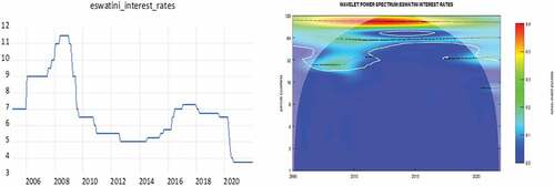
In this section, we present the WPS analysis on the individual interest rate and inflation series for all SACU countries using the “WaveComp” package in R. The WPS captures the distribution of the energy contained within the time series across a time-frequency space and informs us how much frequency band has contributed to energy of the series at different time periods. Henceforth, the periodicities in the time series and their duration can be easily discerned using the WPS. This information is presented across two-dimensional heat-maps that measure time along the horizontal axis and the corresponding frequency along the vertical axis. Note that the frequency components have been converted into “time cycles” with longer (shorter) time cycles corresponding to lower (higher) frequency components. The different colour contours within the heat maps measure the strength of variability within the series at different scales and the warmer (cooler) colours indicating stronger (weaker) variation. The white contour lines surrounding the colour contours represent the 95% confidence level whilst the faint inverted U-shaped curve denotes the cone of influence and represents regions where the WPS suffers from edge effects and hence caution is taken in interpreting regions just inside the cone of influence.

Figures 1–5 present the time series plots for the nominal interest rates in the SACU countries on the left side and their corresponding WPS plots on the right side. From the onset it is interesting to note that the interest rate series have similar trends in the time domain as well as in the time-frequency domain for all SACU countries with the exception of Botswana are slightly different. For the case of South Africa, Namibia, Lesotho and Eswatini the WPS shows two dominant frequency bands; one with strong variation (red contour) at frequency cycles of between 100–128 months (8.667–10.667 years) and another with weaker variation (green contour) at cycles of between 32–64 months (2.667–5.3333 years). Notably, some lower frequency components of 32–64 months (2.667–5.333 years) and intermediate frequency cycle of 64–100 months (5.333–8.667 years) are lost between 2012–2016 and yet both of the “lost cycles” are regained after 2016. On the other hand, the WPS for Botswana shows two dominant bands existing between 2005–2012; one with strong variation (red contour) at frequency cycles of between 100–128 months (8.333–10.667 years) and another frequency band with weaker variation (green contour) at cycles of between 32–64 months (2.667–5.333 years). After 2012 the 32–64 frequency band is lost and only the lower-frequency component of 100–128 months remains but with weak variability (green contour).

Figure 1. Time series and WPS plot for interest rates in South Africa.

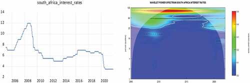
Figure 2. Time series and WPS plot for interest rates in Botswana.

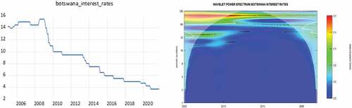
Figure 3. Time series and WPS plot for interest rates in Lesotho.

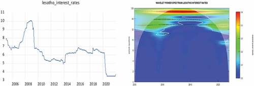
Figure 4. Time series and WPS plot for interest rates in Namibia.

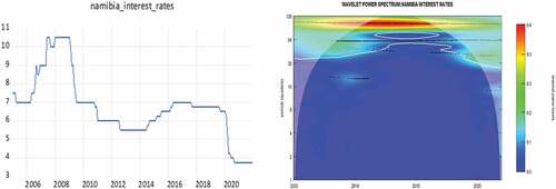
Figure 5. Time series and WPS plot for interest rates in Eswatini.

Notes: From Figures 1 to 5 the time series is shown on the left and the WPS on the right. From the WPS the white contour line represents the significance level. The strength of variation within the series ranges from blue colour (weak correlation) to red colour (strong correlation).

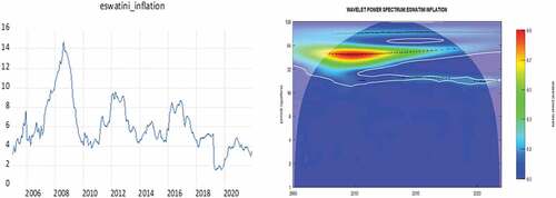
Figures 6–10 present the time series plots for inflation rates in the SACU countries on the left side and their corresponding WPS plots on the right side. Similar to the case for interest rates, we find that the size, strength and duration of the periodicities detected within the inflation time series, as measured by the WPS, are similar for all SACU nations except Botswana. For inflation in South Africa, Namibia, Lesotho and Eswatini, the WPS shows three frequency bands in the data, one with strong variation (red contour) at 40–64 months (3.333–5.333 years), another with weaker variation (green contour) at lower frequencies of 64–100 months (5.333–8.333 years) and a last also with weaker variation (green contour) at higher frequencies of 32–40 months (2.667–3.333 years). However, after 2012 the later two frequency bands at 32–40 months and 64–100 months are lost, the strength of variation in the frequency band at 40–64 months is weakened, and a new frequency band is gained at 20–32 month (1.667–2.667 years) cycles. For the case of Botswana, the WPS shows three dominant frequency bands, one with strong variation (red contour) at 28–36 months (2.333–3 years), another with weaker variation (green contour) at lower frequencies of 36–40 months (3–3.333 years) and a last with weaker variation (green contour) at higher frequencies of 20–28 months (1.667–2.333 years). Notably, all three frequency bands quickly lose their relevance after 2012 and some weak high frequency variation at 20–28 months arise after 2019.

Figure 6. Time series and WPS plot for inflation in South Africa.

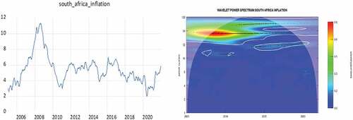
Figure 7. Time series and WPS plot for inflation in Botswana.

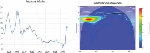
Figure 8. Time series and WPS plot for inflation in Lesotho.

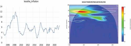
Figure 9. Time series and WPS plot for inflation in Namibia.

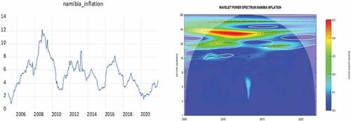
Figure 10. Time series and WPS plot for inflation in Eswatini.

Notes: From Figures 6 to 10 the time series is shown on the left and the WPS on the right. From the WPS the white contour line represents the significance level. The strength of variation within the series ranges from blue colour (weak correlation) to red colour (strong correlation).

4.3. Wavelet coherence analysis

In this section, we present the findings from our wavelet coherence analysis which analyses the co-movement between nominal interest rates and inflation (expectations) for SACU countries across a time-frequency domain. All computations have been conducted using the “WaveComp” package in R. For comparative sake, we present the individual cross-sectional time series plots of nominal interest rates and inflation for the 5 SACU countries in Figure 13. The main wavelet coherence plots are reported in Figures 11-16 describe the co-movement between interest rates and inflation in time-frequency domain. The intensity of synchronization between the series is measured by the colour contours in the heatmaps, with the red contours implying a “one-for-one” co-movement between the series (full fisher effect) at certain periodicities across different time periods whilst less warm colour contours indicate a partial Fisher effect. The faint white lines surrounding the colour contours indicate the 5% significance level whereas the inverted U-shaped curve is the cone of influence which represent the edge effects.

Figure 11. Time series and wavelet coherence plot for inflation and interest rates in South Africa.

Figure 12. Time series and wavelet coherence plot for inflation and interest rates in Botswana.

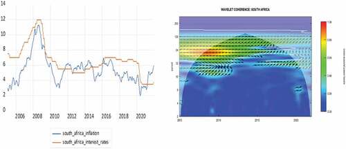
Figure 13. Time series and wavelet coherence plot for inflation and interest rates in Lesotho.

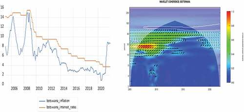
Figure 14. Time series and wavelet coherence plot for inflation and interest rates in Namibia.

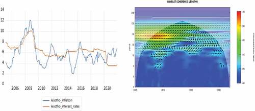
Figure 15. Time series and wavelet coherence plot for inflation and interest rates in Eswatini.

Notes: From Figures 12-16 the time series co-movement is shown on the left and the wavelet coherence plots on the right. From the wavelet plots the white contour line represents the significance level. The power of correlation ranges from blue colour (weak correlation) to red colour (strong correlation). The arrow notations, $\uparrow$, $\nearrow$, $\to$, $\searrow$, ($\downarrow$, $\swarrow$, $\leftarrow$, $\nwarrow$) indicate that a positive (negative) relationship between the series. The arrow notations,$\uparrow$, $\nearrow$, $\to$, $\swarrow$,$\leftarrow$, ($\searrow$,$\downarrow$,$\nwarrow$) indicate that nominal interest rates are leading (lagging) inflation rates

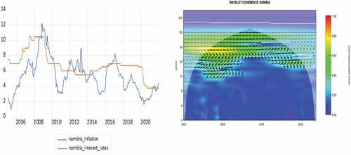
Figure 16. Diagram of phase dynamics.

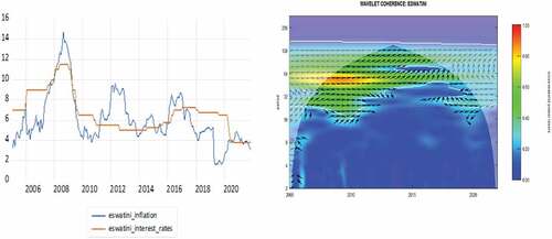
The phase difference dynamics within the wavelet coherence plots are indicated by arrow orientation and provide information on whether the series is in-phase (positively related) or anti-phase (negatively correlated) as well as on the lead-lag synchronization between the series (See, Figure 16 below).

The arrow notations, $\uparrow$, $\nearrow$, $\to$, $\searrow$,indicate that an in-phase (positive) relationship between the series which is consistent with the traditional Fisher effect, whilst the arrow notations, $\downarrow$, $\swarrow$, $\leftarrow$, $\nwarrow$ indicate that an anti-phase (negative) relationship between the series which is consistent with the Mundell-Fisher effect. Moreover, the arrow notations, $\uparrow$, $\nearrow$, $\to$, $\swarrow$,$\leftarrow$, indicate that nominal interest rates are leading inflation rates, which is in line with traditional theory. On the other hand, the arrow notations, $\searrow$,$\downarrow$,$\nwarrow$, indicate that inflation expectations are leading nominal interest rates which is consistent with causal dynamics underlying the Neo-Fisherian effect (Amano et al., 2016; Cochrane, 2016; Uribe, 2018; Williamson, 2018).

It is interesting to note that the synchronization between nominal interest rates and inflation across a time-frequency plane exhibit similar dynamic for all SACU countries. Firstly, we observe “one-for-one” synchronizations (red contours) in all SACU countries around the period of 2005–2012 at lower cyclical frequencies of 40–64 months (3.333–5.333 years) cycles for South, Africa, Lesotho, Namibia and Eswatini and higher cyclical frequencies of 28–32 months (2.333–2.667 years) for Botswana. Secondly, between 2012–2016 the higher frequency components begin to be eliminated and only weaker (green contour) lower-frequency components of 64–128 months (5.333 years–10.667 years) for cycles for South, Africa, Lesotho, Namibia and Eswatini and lower cyclical frequencies of 28–32 months (2.333–2.667 years) for Botswana. Thirdly, from 2016 onwards, the “lost” higher frequencies components are regained albeit the observed synchronization turn extremely weak (light blue contours). Lastly, judging by the arrow orientation, we conclude that synchronization between the series is generally in-phase with nominal interest rates leading inflation expectations as insinuated by the traditional Fisher effect. However, some exception is warranted for the 2007–2012 period in South Africa, Lesotho, Namibia and Eswatini at higher frequency oscillations of 20–32 month (1.667–2.667 year) cycles where inflation rates lead nominal interest rates (see arrows $\searrow$).

4.4. Further discussion of findings

In this section of the paper, we present further discussions based on the findings obtained from the WPS for interest rates and inflation as well as from the wavelet coherence analysis between the series. We further contextualize our findings in context of those obtained in previous SACU-related literature and highlight the new insights provided by our study.

Firstly, the findings from the WPS of the interest rates and inflation series highlight some stylized facts on policy co-ordination and inflation variability along a time-frequency plane. For instance, we observe similar interest rate movement amongst all SACU countries except Botswana which is not surprising considering that Botswana is not part of the CMA and hence policymakers in Botswana do not prioritize mimicking interest rates movements of the SARB. The WPS shows that despite similar sharp cyclical variability being found in interest rates around the global financial crisis in all SACU countries, only Botswana shows low-frequency variation in periods subsequent to the crisis, whereas in the remaining countries (i.e. South Africa, Lesotho, Namibia, Eswatini) interest rates experience additional sharp cyclical variation during the coronavirus pandemic. On the other hand, the WPS of the inflation rates in all SACU countries show similar strong cyclical viability around the global financial crisis and subsequent to the crisis, cyclical variation disappears in the Botswana series whereas for the remaining SACU countries high-frequency oscillations become dominant during the 2014–2016 oil gut period and the more recent COVID-19 pandemic.

Secondly, the findings from the wavelet coherence analysis provides a more comprehensive narrative on the co-movement between the nominal interest rates and inflation expectations in SACU countries between 2005 and 2021. For starters, we find that the traditional Fisher effect is time-varying, with a full Fisher effect being established during periods covering the global financial crisis of 2007–2008 and the global recession of 2009–2010 at frequency oscillations of approximately 64 months (5.333 years) for CMA members and at higher frequency oscillations of 32 months (2.667 years) for Botswana. However, subsequent to these crises periods we observe a partial Fisher effect which are at first dominated by low frequency bands and yet towards the oil gut period of 2016–2019 as well as the more recent COVID-19 pandemic higher frequency components become more dominant. It is also interesting to note that during periods which contain higher frequency oscillations coincide with periods in which the policy rate is higher than the inflation rate i.e. positive real interest rate. For instance, during the global financial crisis of 2007–2009 as well as during the oil gut period of 2016–2019, most SACU countries recorded positive interest rates. Moreover, it is important to point that with the exception of Botswana, the remaining SACU countries recorded the most inconsistent positive real interest rates during 2012–2016 period which is characterized by low-frequency synchronizations amongst the series. For the case of Botswana, interest rates have been positive throughout our sample period until the COVID-19 era when they only more recently turned negative.

Thirdly, from an empirical perspective, our findings bind together “bits and pieces” of empirical evidences from previous studies and also separate the “wheat from the chaff”. For South Africa, our findings simultaneously concur with those of Wesso (2000), Mitchell-Innes et al. (2007), Nemushungwa (2016) who find partial Fisher effects as well as those of Phiri and Lusanga (2011) and Phiri and Mbekeni (2021) who find that the Fisher effect is stronger during periods of rising inflation which occurred in the pre-crisis period. Moreover, our findings are consistent with those presently recently by Phiri (2021) which find reverse causality (i.e. NeoFisherian dynamics) for the South African economy. However, our findings are not in line with those of Yaya (20,150 and Bahmani-Oskooee et al. (2016) who fail to find evidence of Fisher effect for South Africa. Similarly, for Botswana, Lesotho and Eswatini, our findings align with those of Bosupeng (2015) and Khumalo et al. (2017) who finds evidence of Fisher effect in the mentioned countries, respectively. However, our findings are at odds with those of Peyavali and Sheefeni (2013) who fail to find any significant Fisher effects for Namibia whilst our study manages to verify these effects.

5. Conclusion

This study examines the Fisher effect for SACU countries using a set of continuous wavelet tools which allow us to investigate the co-movement between nominal interest rates and inflation expectations over a time-frequency domain. This differs from conventional methods used in the current literature which depend on time-domain estimation techniques which ignore important frequency oscillations in the data. The wavelet tools, such as WPS, CWPS and phase dynamics, present a formidable unified analytical framework which simultaneously addresses empirical inconsistencies and puzzles existing in the Fisher relationship.

The wavelet tools allow us to examine the co-movement between nominal interest rates and inflation expectations in SACU countries from 5 dimensions. Firstly, from a time perspective, we find that there has been continuous co-movement between the series in the post-2000 period for all countries. Secondly, from a frequency perspective, we find that higher frequency co-movements are dominant during the global financial crisis of 2009, global recession period of 2009–2010, oil gut period of 2014–2017 and the more recent COVID-19 pandemic whilst lower frequency synchronizations are dominant during lower inflation periods of 2012–2015. Thirdly, from a magnitude perspective, we find that the Fisher effect is most dominant during the global financial crisis whilst weakening in the post-crisis period. Fourthly, from a phase perspective, we find that the series are in-phase (positively co-related). Lastly, from a lead-lag perspective, we find that whilst nominal interest rates lead inflation expectations at low frequencies, as is consistent with traditional theory, at higher frequency components around the global financial crisis, we find evidence of reverse lead-lad dynamics which is conformity to NeoFisherian dynamics.

Overall, our study has important academic contributions and policy implications. From an empirical perspective, our study is the first to apply CWTs in investigating the Fisher effect within a bi-variate framework. Our study shows that these methods are particularly useful in binding together seemingly contradictory theoretical and empirical evidence presented in previous studies which rely on time-domain econometric techniques and encourage future studies. From a policy perspective, our finding show that the Fisher effect seems to hold the most during periods of crisis when policymakers are behaving most aggressive to unprecedent burst of inflation and we find that high frequency synchronization allows Central Banks to keep their policy rates above inflation and maintain a positive interest rate. Moreover, during periods of low-inflation such as between 2012–2016, the Fisher effect weakens, higher frequency synchronizations lost their relevance in favour of lower frequency oscillations when policymakers behaved very conservative and even allowed real interest rates to turn negative. Notably, during the ongoing COVID-19 crisis period, we observe some higher frequency oscillations indicating a partial Fisher effects during this crisis period. However, based on our findings, policymakers in SACU countries need to ensure a Full Fisher effect during the recent periods of increasing inflation during times of pandemic crisis and policymakers need to be more aggressive in their approach to policy conduct in order to combat rising inflation whilst keeping real interest rates positive, thus protecting the finances of savers and investors in financial institutions. This policy advice is more relevant for Botswana policymakers who have been very conservative with their interest rates and have not increased them over the last 10 years despite experiencing significant increases in recent inflation rates. The remaining SACU countries are dependent on decisions taken by the SARB and therefore the recent increases in interest rates announced by the SARB in early 2022 are a step in the direction and will have spillover effects into policy decisions taken by the other members of the CMA.

Disclosure statement

No potential conflict of interest was reported by the author(s).

Additional information

Funding

The authors received no direct funding for this research.

References

- Adil, M., Danish, S., Bhat, S., & Kamaiah, B. (2020). Fisher effect: An empirical re-examination in case of India. Economics Bulletin, 40(1), 262–19. http://www.accessecon.com/Pubs/EB/2020/Volume40/EB-20-V40-I1-P24.pdf
- Aguiar-Conraria, L., Martins, M., & Soares, M. (2014). The continuous wavelet transform: Moving beyond uni- and bivariate analysis. Journal of Economic Dynamics & Control, 28(2), 344–375. https://doi.org/10.1111/joes.12012
- Aguiar-Conraria, L., Martins, M., & Soares, M. (2020). Okun’s law across time and frequencies. Journal of Economic Dynamics & Control, 116, e103897. https://doi.org/10.1016/j.jedc.2020.103897
- Amano, R., Carter, T., & Mendes, R. (2016). A primer on Neo-Fisherian economics. Bank of Canada Staff Analytical Notes, 16–14. https://www.bankofcanada.ca/wp-content/uploads/2016/09/san2016-14.pdf
- Amsler, C. (1986). The Fisher effect: Sometimes inverted, sometimes not? Southern Economic Journal, 52(3), 832–835. https://doi.org/10.2307/1059278
- Atkins, F. (1989). Co-integration, error correction and the Fisher effect. Applied Economics, 21(12), 1611–1620. https://doi.org/10.1080/758531695
- Aziakpono, M. (2008). Financial and monetary autonomy and interdependence between South Africa and the other SACU countries. South African Journal of Economics, 76(2), 189–211. https://doi.org/10.1111/j.1813-6982.2008.00173.x
- Bahmani-Oskooee, M., Li, J., & Chang, T. (2016). Revisiting Fisher equation in BRICS countries. Journal of Global Economics, 4(3), 1–3. https://doi.org/10.4172/2375-4389.1000210
- Barksy, R., & de Long, J. (1991). Forecasting pre-World War 1 inflation: The Fisher effect and the gold standard. The Quarterly Journal of Economics, 106(3), 815–836. https://doi.org/10.2307/2937928
- Barsky, R. (1987). The Fisher hypothesis and the forecastability and persistence of inflation. Journal of Monetary Economics, 19(1), 3–24. https://doi.org/10.1016/0304-3932(87)90026-2
- Bayat, T., Kayhan, S., & Tasar, I. (2018). Re-visiting fisher effect for fragile five economies. Journal of Central Banking Theory and Practice, 7(1), 203–218. https://doi.org/10.2478/jcbtp-2018-0019
- Berument, H., & Froyen, R. (2021). The Fisher effect on long-term U.K. interest rates in alternative monetary regimes: 1844-2018. Applied Economics, 53(33), 3795–3809. https://doi.org/10.1080/00036846.2021.1886239
- Berument, H., & Jelassi, M. (2002). The Fisher hypothesis: A multi-country analysis. Applied Economics, 34(13), 1645–1655. https://doi.org/10.1080/00036840110115118
- Bosupeng, M. (2015). The fisher effect using differences in the deterministic term. International Journal of Latest Trends in Finance and Economic Sciences, 4(5), 1031–1040.
- Cai, Y. (2018). Testing the Fisher Effect in the US. Economics Bulletin, 38(2), 1014–1027. http://www.accessecon.com/Pubs/EB/2018/Volume38/EB-18-V38-I2-P97.pdf
- Carmicheal, J., & Stebbing, P. (1983). Fisher’s paradox and the theory of interest. American Economics Review, 73(4), 619–630. https://www.jstor.org/stable/1816562
- Choudhry, T., Placone, D., & Wallace, M. (1991). Changes in the Fisher effect in the 1980ʹs: Evidence from various models. Journal of Economics and Business, 43(1), 59–68. https://doi.org/10.1016/0148-6195(91)90006-I
- Choudhury, T. (1997). Cointegration analysis of the inverted Fisher effect: Evidence from Belgium, France and Germany. Applied Economics Letters, 4(4), 257–260. https://doi.org/10.1080/758518506
- Christopoulos, D., & Leon-Ledesma, M. (2007). A long-run non-linear approach to the Fisher effect. Journal of Money, Credit, and Banking, 39(2/3), 543–559. https://doi.org/10.1111/j.0022-2879.2007.00035.x
- Cochrane, J. (2016), “Do higher interest rates raise or lower inflation?”, Hoover Institute Working Paper, February.
- Crowder, W., & Hoffman, D. (1996). The long-run relation between nominal interest rates and inflation: The Fisher equation revisited. Journal of Money, Credit, and Banking, 28(1), 102–118. https://doi.org/10.2307/2077969
- Crowley, P., & Hudgins, D. (2021). Is the Taylor rule optimal? Evaluation using wavelet-based control model. Applied Economic Letters, 28(1), 54–60. https://doi.org/10.1080/13504851.2020.1730752
- Darby, M. (1975). The financial and tax effects of monetary policy on interest rates. Economic Inquiry, 13(2), 266–276. https://doi.org/10.1111/j.1465-7295.1975.tb00993.x
- Evans, M., & Lewis, K. (1995). Do expected shifts in inflation affect estimates of the long-run fisher relation? Journal of Finance, 50(1), 225–253. https://doi.org/10.1111/j.1540-6261.1995.tb05172.x
- Fahmy, Y., & Kandil, M. (2003). The Fisher effect: New evidence and implications. International Review of Economics and Finance, 12(4), 451–465. https://doi.org/10.1016/S1059-0560(02)00146-6
- Fama, E. (1975). Short-term interest rates as predicators of inflation. The American Economics Review, 65(3), 269–282. https://www.jstor.org/stable/1804833
- Feldstein, M. (1976). Inflation, income taxes, and the rate of interest: Theoretical analysis. American Economic Review, 66(5), 809–820. https://www.jstor.org/stable/1827493
- Fisher, I. (1930). “The Theory of Interest”. MacMillan.
- Gallagher, M. (1986). The inverted Fisher hypothesis: Additional evidence. American Economic Review, 76(1), 247–249. https://www.jstor.org/stable/1804143
- Garcia, P., & Zapata, H. (1991). Co-integration, error correction and the Fisher effect: A clarification. Applied Economics, 23(8), 1367–1368. https://doi.org/10.1080/00036849100000058
- Goupillaud, P., Grossmann, A., & Morlet, J. (1984). Cycle-octave and related transforms in seismic signal analysis. Geoexploration, 23(1), 85–105. https://doi.org/10.1016/0016-7142(84)90025-5
- Granville, B., & Mallick, S. (2004). Fisher hypothesis: UK evidence over a century. Applied Economic Letters, 11(2), 87–90. https://doi.org/10.1080/1350485042000200169
- Grossmann, A., & Morlet, J. (1984). Decomposition of Hardy functions into square integrable wavelets of constant shape. SIAM Journal of Mathematical Analysis, 15(4), 723–736. https://doi.org/10.1137/0515056
- Gylfason, T., Tómasson, H., & Zoega, G. (2016). Around the world with Irving Fisher. North American Journal of Economics and Finance, 36, 232–243. https://doi.org/10.1016/j.najef.2016.01.004
- Hasan, H. (1999). Fisher Effect in Pakistan. The Pakistan Development Review, 38(2), 153–166. https://doi.org/10.30541/v38i2pp.153-166
- Haug, A. (2014). On real interest rate persistence: The role of breaks. Applied Economics, 46(10), 1058–1066. https://doi.org/10.1080/00036846.2013.864043
- Jochmann, M., & Koop, G. (2014). Regime-switching cointegration. Studies in Nonlinear Dynamics and Econometrics, 19(1), 35–48. https://doi.org/10.1515/snde-2012-0064
- Khumalo, C., Mutambara, E., & Akwesi Assensoh- Kodua, A. (2017). Relationship between inflation and interest rates in Swaziland revisited. Banks and Bank Systems, 12(4), 218–226. https://doi.org/10.21511/bbs.12(4-1).2017.10
- Kim, D., Lin, S., Hsieh, J., & Suen, Y. (2018). The Fisher equation: A nonlinear panel data approach. Emerging Markets and Finance, 54(1), 162–180. https://doi.org/10.1080/1540496X.2016.1245138
- King, R., Plosser, C., Stock, J., & Watson, M. (1991). Stochastic trend and economic fluctuations. American Economic Review, 81(4), 819–840. https://www.jstor.org/stable/2006644
- Koustas, Z., & Lamarche, J. (2007). Evidence of nonlinear mean reversion in real interest rate. Applied Economics, 42(2), 237–248. https://doi.org/10.1080/00036840701579242
- Koustas, Z., & Serletis, A. (1999). On the Fisher effect. Journal of Monetary Economics, 44(1), 105–130. https://doi.org/10.1016/S0304-3932(99)00017-3
- Krüger, J., & Neugart, M. (2020). Dissecting Okun’s law beyond time and frequency. Applied Economics Letters, 28(20), 1744–1749. https://doi.org/10.1080/13504851.2020.1853664
- Maozzami, B. (1990). Interest rates and inflationary expectations: Long-run equilibrium and short-run adjustment. Journal of Banking and Finance, 14(6), 1163–1170. https://doi.org/10.1016/0378-4266(90)90007-O
- Million, N. (2004). Central bank’s interventions and the Fisher Hypothesis: A threshold cointegration investigation. Economic Modelling, 21(6), 1051–1064. https://doi.org/10.1016/j.econmod.2004.03.002
- Mishkin, F. (1992). Is the Fisher effect for real? A re-examination of the relationship between inflation and interest rates. Journal of Monetary Economics, 30(2), 195–215. https://doi.org/10.1016/0304-3932(92)90060-F
- Mishkin, F. (1995). Symposium on monetary transmission mechanism. Journal of Economic Perspectives, 9(4), 2483–2492. https://doi.org/10.1257/jep.9.4.3
- Mishkin, F., & Simon, J. (1995). An empirical examination of the Fisher effect in Australia. Economic Record, 71(3), 217–229. https://doi.org/10.1111/j.1475-4932.1995.tb01889.x
- Mitchell-Innes, H., Aziakpono, M., & Faure, A. (2007). Inflation targeting and the Fisher effect in South Africa: An empirical investigation. South African Journal of Economics, 75(4), 693–707. https://doi.org/10.1111/j.1813-6982.2007.00143.x
- Nchake, M., Edwards, L., & Rankin, N. (2018). Closer monetary union and product market integration in emerging economies: Evidence from the common Monetary Area in Southern Africa. International Review of Economics and Finance, 54, 154–164. https://doi.org/10.1016/j.iref.2017.08.004
- Nemushungwa, A. (2016), ‘An empirical study of Fisher effects and the dynamic relation between nominal interest rates and inflation in South Africa”, AP16 Mauritius Conference. Ebene-Mauritius: Global Bizresearch.
- Nusair, S. (2008). Testing for the Fisher hypothesis under regime shifts: An application to Asian countries. International Economic Journal, 22(2), 273–284. https://doi.org/10.1080/10168730802095660
- Ongan, I., & Gocer, S. (2018). Interest rates, inflation and partial Fisher effects under nonlinearity: Evidence from Canada. Economics Bulletin, 38(4), 1957–1969. http://www.accessecon.com/Pubs/EB/2018/Volume38/EB-18-V38-I4-P179.pdf
- Ongan, I., & Gocer, S. (2020). Testing fisher effect for the USA: Application of nonlinear ARDL model. Journal of Financial Economic Policy, 12(2), 293–304. https://doi.org/10.1108/JFEP-09-2018-0127
- Ozcan, B., & Ari, A. (2017). Does the Fisher hypothesis hold for the G7? Evidence from the panel cointegration test. Economic Research – Ekonomska Istrazivanja, 28(1), 271–283. https://doi.org/10.1080/1331677X.2015.1041777
- Paleologos, J., & Georgantelis, S. (1999). Does the Fisher effect apply in Greece? A cointegration analysis. Economia Internazionale/International Economics, 52(2), 229–243. https://www.researchgate.net/publication/46558180_Does_the_Fisher_Effect_Apply_in_Greece_A_Cointegration_Analysis
- Paul, T. (1984). Interest rates and the Fisher effect in India. Economics Letters, 14(1), 17–22. https://doi.org/10.1016/0165-1765(84)90022-3
- Payne, J., & Ewing, B. (1997). Evidence from lesser developed countries on the fisher hypothesis: A cointegration analysis. Applied Economics Letters, 4(11), 683–687. https://doi.org/10.1080/758530649
- Pelaez, R. (1995). The fisher effect: Reprise. Journal of Macroeconomics, 17(2), 333–346. https://doi.org/10.1016/0164-0704(95)80105-7
- Peyavali, J., & Sheefeni, S. (2013). Testing for the Fisher Hypothesis in Namibia. Journal of Emerging Issues in Economics, Finance and Banking, 2(1), 571–582. https://www.researchgate.net/publication/308202541_Testing_for_the_Fisher_Hypothesis_in_Namibia
- Phiri, A. (2021). Is NeoFisherism ‘alive’ in South Africa? A frequency domain causality approach. Macroeconomics and Finance in Emerging Market Economies, 14(2), 142–156. https://doi.org/10.1080/17520843.2020.1796732
- Phiri, A., & Lusanga, P. (2011). Can asymmetries account for the empirical failure of the Fisher effect in South Africa? Economics Bulletin, 31(3), 1968–1979. http://www.accessecon.com/Pubs/EB/2011/Volume31/EB-11-V31-I3-P178.pdf
- Phiri, A., & Mbekeni, L. (2021). Fisher hypothesis, survey-base expectations, and asymmetric adjustments: Empirical evidence from South Africa. International Economics and Economic Policy, 18(4), 825–846. https://doi.org/10.1007/s10368-021-00498-2
- Rose, A. (1988). Is the real interest rate stable? Journal of Finance, 43(5), 1095–1112. https://doi.org/10.1111/j.1540-6261.1988.tb03958.x
- Rua, A. (2012, September). Wavelet in Economics. Banco de Portugal Economic Bulletin, 71–79. https://www.bportugal.pt/sites/default/files/anexos/papers/ab201208_e.pdf
- Rua, A., & Nunes, L. (2009). International co-movement of stock market returns: A wavelet analysis. Journal of Empirical Finance, 16(4), 632–639. https://doi.org/10.1016/j.jempfin.2009.02.002
- Sánchez-Fung, J. (2019). Interest rates, inflation, and the Fisher effect in China. Macroeconomics and Finance in Emerging Market Economies, 12(2), 124–133. https://doi.org/10.1080/17520843.2019.1592206
- Sugita, K. (2017). Non-linear analysis of the Fisher effect: In the case of Japan. International Journal of Economics and Finance, 9(11), 1–9. https://doi.org/10.5539/ijef.v9n11p1
- Tiwari, A., Cunado, J., Gupta, R., & Wohar, M. (2019). Are stock returns an inflation hedge for the UK? Evidence from a wavelet analysis using over three centuries of data. Studies in Nonlinear Dynamics and Econometrics, 23(3), 20170049. https://doi.org/10.1515/snde-2017-0049
- Torrence, C., & Compo, G. (1998). A practical guide to wavelet analysis. Bulletin of American Meteorological Society, 79(1), 61–78. https://doi.org/10.1175/1520-0477(1998)079<0061:APGTWA>2.0.CO;2
- Toyoshima, Y., & Hamori, S. (2011). Panel cointegration of the Fisher effect: Evidence from the US, the UK and Japan. Economics Bulletin, 31(3), 2674–2682. http://www.accessecon.com/Pubs/EB/2011/Volume31/EB-11-V31-I3-P240.pdf
- Uribe, M. (2018), “The Neo-Fisher effect: Econometric evidence from empirical and optimizing models”, NBER Working Paper No. 25089, September.
- Wallace, M., & Warner, J. (1993). The Fisher effect and the term structure of interest rates: Test of cointegration. The Review of Economics and Statistics, 75(2), 320–324. https://doi.org/10.2307/2109438
- Weidmann, J. (1997 January). New hope for the Fisher effect? A re-examination using threshold co-integration. University of Bonn Discussion, Paper B-385.
- Wesso, G. (2000, June). Long-term yield bonds and future inflation in South Africa: A vector error-correction analysis. Quarterly Bulletin. Pretoria: South African Reserve Bank. https://www.resbank.co.za/content/dam/sarb/publications/quarterly-bulletins/articles-and-notes/2000/4790/Article---Long-term-bond-yields-and-future-inflation-in-SA.pdf
- Williamson, S. (2018). Inflation control: Do Central Banks have it right? Federal Reserve Bank of St. Louis, 100(2), 127–150. http://dx.doi.org/10.20955/r.2018.127-50
- Wong, K., & Wu, H. (2003). Testing Fisher hypothesis in long horizons for G7 and eight Asian countries. Applied Economic Letters, 10(14), 917–923. https://doi.org/10.1080/1350485032000158645
- Yaya, K. (2015). Testing the long-run Fisher effect in selected African countries: Evidence from ARDL bounds test. International Journal of Economics and Finance, 7(12), 168. https://doi.org/10.5539/ijef.v7n12p168