Predictive directional measurement volatility spillovers between the US and selected Asian Pacific countries

Abstract

Since portfolio management relies on the association of portfolio diversification, analyzing the spillover between the United States (US) and Asian-Pacific financial markets has become more critical. If Asian stock markets have low or negative correlations with each other and/or the US market, global investors may benefit from diversification. This study examines the return and volatility spillover between the S&P 500 and 12 Asian stock markets using weekly data from January 2000 to February 2020. DECO-GARCH models are employed to measure volatility transmission between markets. A generalized VAR, variance decomposition, and spillover index is employed to investigate the directional spillover across the sample, allowing for a focus on the interdependence of the conditional returns, conditional volatility, and conditional correlations between the stock markets. Hedge ratios and portfolio weights use to examine the results’ implications for international portfolio diversification and risk management. The study calculates the effectiveness of hedging equities portfolios between markets, using the beta hedge approach to minimize the risk of this stock market index returns portfolio. The results demonstrate that Hong Kong and Singapore have a clear direction of a return to other stock markets, whereas China has a clear net recipient. The US market does not provide a superior hedging ratio for Asia-Pacific nations. For other stock markets, India, Hong Kong, and New Zealand have the best hedge ratios, portfolio weights, and hedging efficacy. Finally, this research raised the information linked between the stocks market index and can also apply to improve international portfolio by re-considering the cheapest hedging markets and improving the trading strategies in international markets.

Keywords:

• Asia Pacific stock markets
• financial market contagion
• directional spillover index
• hedging equity portfolios
• DECO-GARCH model

Jel classifications:

• C58
• F36
• G1
• G11
• G17

1. Introduction

How the stock market responds to information transmission across financial marketplaces determines how investors might recover their investment plans to maximize profits. For example, investors may reduce risk and build portfolios by including the lowest number of linked shares across markets. Since the 1990s, global financial instability has compelled investors and portfolio managers to reduce risk by diversifying portfolios. That has increased the importance of estimating the depth and length of volatility spillovers destabilizing other markets. Spillover analysis identifies shock sources and shock takers. The leading financial markets found that it influences other financial markets; for example, it is more probable that the United States stock markets would be spillover sources on different financial markets (Cheung et al., 2007; Granger, 1986; Hamao et al., 1990; King & Wadhwani, 1990; Yilmaz, 2010). Lately, Lien et al. (2018) observed that volatility spillovers from the US markets to foreign markets are unidirectional only during financial crises. Instead, research shows that stock market shocks originate in the US and extend to other financial markets.

Previous studies have revealed that the US stock markets have detrimental effects on other financial markets. While many economic indices have improved since the financial crisis in 2007, stock markets have been among the first to benefit, as risk aversion and interest rates have reduced, and investors seek higher returns and reinvest their capital in the stock market. Furthermore, evaluating the spillover between the US and Asian-Pacific financial markets for portfolio diversification is becoming more vital since portfolio output depends on the association between portfolio resources. Indeed, if Asian-Pacific stock markets have negative or low correlations between each other and/or with the US market, it provides diversification investment opportunities for international investors.

The Asian Financial Crisis of 1997–98 and the Great Recession sparked a regional and country-level financial industry reform agenda. As a result, a rapid shift in its financial markets’ institutional structure has occurred. Since the beginning of this century, these markets have grown significantly, with several regional markets showing extraordinary depth and resistance to external shocks. There has also been an increase in equity markets and a more comprehensive range of investors. The latest Bank for International Settlements (BIS) report also shows that Hong Kong, Singapore, Sydney, and Tokyo’s foreign currency and derivative markets are expanding.

Nowadays, Asia-Pacific nations constitute the world’s largest trading union by value, ranking first in exports and second in imports with 5.3 trillion US dollars (2019), 30 percent of the world’s GDP, which is greater than the sum of the US and EU trade, or 4.3 trillion US dollars. The Regional Comprehensive Economic Partnership (RCEP) countries along the endorsement process in the next 10 to 20 years will also become the world’s largest market with a population of 2.3 billion people, of which 69 percent will come from the world’s three leading economies: China, Japan, and South Korea which will be associate for the first time in a Free Trade Agreement (FTA), comprising 1.6 billion people and accounting for 80 percent of their total GDP.

The Asia-Pacific market presents a bright outlook for the next decade, with a consistent increase in economic development that is 2 to 3 times the EU or US growth rate, with a predicted average growth of 0.2 percent per partner nation every year by 2031. Due to the significance of intraregional trade flows and investments, the simplification of procedures and laws, rules, and regulations. Through economic or technical exchanges, interregional investments are promoted in activities with reciprocal advantages to strengthen regional or global linkages. For instance, Japan’s investments with China have reached 38.6 percent of its total investments, 397.07 billion, according to estimates from the World Bank from January to April 2021.

The critical contribution of this study is to examine whether or not leading stock markets, such as the US market, impact the performance of other markets across more extended periods and larger sample sets. Since portfolio production relies on the association of portfolio resources, analyzing the spillover between the US and Asia-Pacific financial markets has become more critical. If Asian stock markets have low or negative correlations with each other and/or with the US market, foreign investors may benefit from diversification. More precisely, this study examines dynamic spillovers between the US market and selected 12 Asian-Pacific countries from 2000 to 2020, including Australia (AUS), China (CHN), Hong Kong (HKG), India (IND), Japan (JPN), Malaysia (MYS), New Zealand (NZL), the Philippines (PHL), Singapore (SGP), South Korea (KOR), Taiwan (TWN), and Thailand (THA). Engle and Kelly (2012) dynamic equicorrelation (DECO) specification and generalized autoregressive conditional heteroscedasticity (GARCH) model, Diebold and Yilmaz (2012), are used to examine the path and magnitude of spillovers.

Second, we introduced a DECO-specific GARCH model. However, this causality varies continually, streamlining the log probability of high-dimensional return estimation. DECO is not replacing Engle’s (2002) traditional dynamic conditional correlation (DCC) model. Compared to the DCC model, DECO utilizes additional data to analyze the changing correlations across returns, decreasing the correlation measurement disturbance. Thus, GARCH models are essential to comprehending the relationship between co-volatilities.

Diebold and Yilmaz’s (2012) spillover index focuses on the prediction-error variance decomposition technique from a particular vector autoregressive (VAR) specification that invariants prediction-error variance decompositions to changing directions. Therefore, one way to measure the impact of directional spillovers is to calculate their net exposure to the information exchange mechanism of other markets. For example, spillovers between stock markets in Asia and other regions of the world, as well as within Asia, can be detected by measuring directional returns and volatility.

The final contribution examines the net spillovers experienced by each market to evaluate whether or not it has been net beneficiaries or transmitted spillovers over the sample period. Let us look at it from the perspective of actual economic dependency. The discoveries of net return and volatility spillovers enable us to comprehend the direction of data and information transfer and identify the net transformer and net receiver of financial data across the entire Asian-Pacific equity markets. It is advantageous for fund managers to recognize net receivers and transformers to reduce the risk of connectedness in their portfolio diversification, modify their investment strategies within a reasonable timeframe, and improve their investment and hedging financial choices to maximize their returns.

This paper is structured as follows. Section 2 discusses previous research findings, and Section 3 explains the evidence and methodological problems. Section 4 discusses this study’s data, and the analysis presents analytical evidence that assesses our tests’ robustness. Finally, Section 5 gave the conclusion of this research.

2. Literature review

Asset pricing and statistical integration models have been used in previous research to examine the consequences of market integration and diversification. The asset pricing viewpoint defines market integration as consistent pricing across markets for assets with similar risk profiles. If the mean-variance concept holds, securities traded on many integrated markets should cluster together on the same security market line. However, according to the statistical integration model, markets are integrated if securities prices across markets tend to move together over time. The level of foreign market integration has significant ramifications for investors’ investment strategy and capital market efficiency, making this study area increasingly popular in recent years. As market integration increases, the benefits of diversity may diminish. Furthermore, the weak-form market efficiency may be compromised when price series are cointegrated since it implies an error-correcting representation of the security prices (Granger, 1986).

Financial market integration creates a world where returns and volatility are intrinsically linked. Financial markets worldwide, no matter whether they are far from each other, have become increasingly integrated because of the proliferation of digital communications and the liberalization of international trade. The term “spillover” describes the effect of increased connectivity between global financial markets on the spread of newly-emerging information from one country to another. Because of its importance in asset pricing, cost of capital estimation, risk evaluation, and the evaluation of foreign portfolio diversification, this interdependence has garnered the attention of academics.

There are two components to the spillover effect: the return spillover and the volatility spillover. First, information on stock returns and volatilities spreads abroad, illustrating the interconnected nature of financial markets worldwide. Traditionally, stock returns are considered a proxy for the market level. Second, stock volatilities are considered a proxy for market risk. As a result, the mean and variance of asset returns are often used in most portfolio theories to assess the return-to-risk trade-off (Markowitz, 1952).

Five approaches for investigating the spillover effect have been proposed in the empirical literature, assuming statistical integration models. The first approach takes into account the spillover effect by using correlation coefficients, either conditional or unconditional (Reinhart & Calvo, 1996 Forbes & Rigobon, 2002; Hwang, 2014; King & Wadhwani, 1990; Lee & Kim, 1993; Z. Liu et al., 2020; Panda & Nanda, 2018; Zhong & Liu, 2021). The second approach cointegration framework used to measure the spillover impact (Abdulrazzaq et al., 2019; Athari et al., 2021; Cashin et al., 1995; Chou et al., 1994; Gulzar et al., 2019; Hung & Vo, 2021; Kannadas & Viswanathan, 2022; Longin & Solnik, 1995).

The third approach looks at the highest prices in different markets. Using multivariate extreme value theory to measure how excessive stock returns all act together (Athari & Hung, 2022; Baele et al., 2004; Chan et al., 2004; Christensen & Nielsen, 2007; Harrison & Moore, 2009; H. Hong et al., 2002; Hussain et al., 2022; K. Liu et al., 2019; Melvin, 2003; Milunovich & Thorp, 2006; Xiao, 2020). The fourth and perhaps most broadly utilized approach is the VAR plus GARCH model, which can be employed to investigate returns as well as volatility spillovers synchronously (Ahmed et al., 2022; Bekaert & Harvey, 1995; Bekaert & Hodrick, 1992; Campbell & Hamao, 1992; Engle et al., 1990; Eun & Shim, 1989; Hamao et al., 1990; Kondoz et al., 2019; Mathur & Subrahmanyam, 1990; Wang & Liu, 2016). The fifth approach makes use of the spillover index. With its foundation in variance decomposition, this index accurately evaluates the extent to which one market affects another (Bonilla & Sepúlveda, 2011; Diebold & Yilmaz, 2012; Fujiwara & Takahashi, 2012; Gębka, 2012; Kang et al., 2019; Panda et al., 2021).

It is conceivable that location will play a role among the elements that create spillover effects. Recent years have seen a greater focus on developing economies than in the past. Over the last few decades, governments around the globe, but especially in Asia’s financial markets, have altered their practices to make international investment easier. While considering the effects of global and regional shocks, Thomas et al. (2017) examine the developed, developing, and frontier markets in the Asia-Pacific region over the long term. The analysis uses indices of stocks’ weekly closing prices from January 2000 to June 2016. The findings of the Zivot and Andrews unit root test and the Gregory and Hansen cointegration test, China and Thailand, Sri Lanka, and Pakistan markets are reasonably different from the other stock markets in the Asia-Pacific area. Therefore, international investors can benefit from the diversification potential these markets provide. Furthermore, the bidirectional cointegration test results indicate that developing and frontier markets impact developed markets. So, it is safe to assume that the adage “bigger is better” no longer applies in the modern economy.

Over the last several years, ties between China and the Association of Southeast Asian Nations (ASEAN) have grown more robust because of initiatives such as the Belt and Road Initiatives and the creation of the China-ASEAN Free Trade Area. In addition, Chinese and ASEAN stock market contacts have grown due to China’s partial openness of its financial markets to global investors. Uludag and Khurshid (2019) analyze the impact of Chinese stock market volatility on stock markets in the E7 and G7 countries from 1995 to 2015. Based on the generalized VAR-GARCH method applied to daily closing prices. The results show that the volatility of the Chinese stock market considerably affects stock markets in the E7 and G7. Specifically, the stock markets of nations in the same area as China tend to move in tandem. For the E7, the most significant volatility spillover occurs between China and India, whereas for the G7, it occurs between China and Japan. In addition, the optimal weights and hedging ratios analysis indicates that investors should have a greater allocation of equities from G7 nations than E7 countries. As a result, liberalization measures frequently resulted in a higher similarity between regional and global market returns. Therefore, more significant cross-national spillover effects are to be anticipated.

Additionally, using daily data, Zhong and Liu (2021) used multivariate GARCH models to highlight dynamic conditional relationships and the volatility spillovers between the Chinese and five Southeast Asian stock markets from 1994 to 2019. The results show a positive dynamic conditional correlation between China and five Southeast Asian stock markets, which reached its highest point in 2015, just around the time of the Asian financial crisis, the US subprime mortgage crisis, and the stock market decline. While other researches have drawn different results, Chen and Wang (2021) use the Copula-TV-GARCH-CoVaR model and the MES model to examine the interdependence and risk spillover effects between the Chinese and ASEAN-6 stock markets from 2010 to 2021. Except for Vietnam, these stock markets appear to have a dependence pattern. The level of dependency was highest for the pair China and Singapore and lowest for Vietnam and the Chinese stock market.

Moreover, it has demonstrated that the correlation between markets is more significant in times of high volatility than in times of low volatility. As a result, spillover effects might change over time and across different contexts. The financial contagion effect characterizes an increase in the strength of links across markets during a crisis. However, such research has focused on the time-varying nature of market integration by high and low volatility periods (Dungey et al., 2010; Favero & Giavazzi, 2002; Forbes & Rigobon, 2002; M. H. Pesaran & Pick, 2007; Kirikkaleli & Athari, 2020; Kondoz et al., 2021). Xiao (2020) studies the effects of Chinese stock market volatility on major East Asian markets in calm and tumultuous years (2014–2018). He uses the Markov regime-switching model, extreme value theory (EVT), and the Covariance matrix of risk (CoVaR). Using direct CoVaR, he revealed several fascinating findings, including that negative and positive spillovers vary during turbulent and calm times (except for the China-Japan and China-South Korea pairs during the tumultuous period). In addition, indirect data suggest distinct changes between turbulent and calm periods.

While financial crises on a global or regional scale are known to cause spillover effects, there is some evidence that these impacts amplify over specific periods (Baig & Goldfajn, 1999; Caporale et al., 2006; Gulzar et al., 2019; D. Hong et al., 2003; Saleem & Vaihekoski, 2008). Gulzar et al. (2019) investigate the financial cointegration and the spillover effect of the global financial crisis on developing Asian financial markets. They used daily stock returns from 2005–2015, and those returns divide into pre-crisis, crisis, and post-crisis periods. They used the Johansen and Juselius cointegration test, the vector error correction model (VECM), and the GARCH-BEKK model to analyze integration and conditional volatility. They found that the US and emerging stock markets cointegrated over the long run, and cointegration rose following the crisis period. When a shock occurs in the US financial market, it temporarily affects the returns of developing financial markets, as seen by the VECM and the impulse response function. Past shocks and volatility affect selected stock markets more than any other historical period. The only stock markets that experienced cross-market news and volatility spillover effects during the crisis era are the South Korean Stock Price Index and the Indian stock exchange. After the crisis, the information favored the India and Russian stock markets but negatively affected Malaysia and China. Samitas et al. (2022) examine the impact of the recent COVID-19 pandemic on 51 developing and developed stock markets. They find the volatility and the contagion risk in the stock markets during the COVID-19 pandemic by employing dependency dynamics and network analysis on a bivariate basis. Evidence suggests that the shutdown and subsequent transmission of the new coronavirus caused immediate financial contagion.

There is an investigation into the possibility of extreme risk spreading across developed and developing stock markets. Su (2020) investigated significant risk spillover among developed and emerging stock markets employing weekly data from 1998 to February 2017 of the G7 and BRICS stock markets. While specific G7 stock markets did emerge as net transmitters of high-risk spillovers, others did not, and neither did all BRICS stock markets appear as net receivers. The developed stock markets (the UK, Japan, and Italy) are net recipients of average significant risk spillovers. In contrast, Brazil is a giant net transmitter in the emerging market category. While high-risk spillovers between the G7 developed and the BRICS developing stock markets, this was only the case for the pairwise direction spillover.

Moreover, the result revealed that the severe risk spillovers showed substantial evidence of time-variability. In particular, the United States, Germany, France, and Canada were net transmitters of severe risk spillovers. In contrast, the stock markets in the United Kingdom, Italy, and the BRICS countries are net receivers.

The results of other publications, however, differ. Evidence of the “Wall Street Virus,” as Chan et al. (2004) dubbed the spread of instability from the US to Asian markets, was provided. In 2007, Bayoumi and Swiston identified the worldwide financial situation as the primary source of spillovers. The spillovers from the United States to Asian economies have grown in recent decades, according to an IMF (2008) assessment. While China’s financial influence in Asia has grown, Fujiwara and Takahashi (2012) found that the United States was the primary cause of the shifts they saw. Trung (2019) uses a VAR (GVAR) framework to analyze the effects of a US policy uncertainty shock on the rest of the world, with data from 32 countries accounting for even more than 90% of global GDP. We find that shocks to US policy uncertainty have a significant role in causing international business cycle variations. However, the effects of US policy uncertainty (such as monetary policy uncertainty vs. fiscal policy uncertainty) on other nations vary widely depending on the characteristics of the country in question (e.g., level of development, trade and financial openness, and quality of institutions).

While in the Asian region, Kang et al. (2019) analyzed data from 2003–2019, using the dynamic equicorrelation (DECO) model and the spillover index of Diebold and Yilmaz (2012), the results show directional spillovers from world stock markets to ASEAN-5 stock markets are more substantial than in a reverse way. Also, over time, the degree of spillover to global markets varies between the ASEAN-5 stock markets. They corroborate the strength of information transmission during turbulence by verifying an increase in both return and volatility spillovers during financial crises. Jebran et al. (2017) examine the volatility spillover impact among developing Asian markets from January 2001 to December 2013 (using daily data). The EGARCH model results found evidence of volatility spillover between the India and Sri Lankan stock markets in both periods and both directions. They detect bidirectional volatility spillover between the Indian and Sri Lanka stock markets in both sub-periods. Nevertheless, volatility spillover is bidirectional between Hong Kong and India stock markets, Pakistan and India in the pre-crisis era, and Sri Lanka and Pakistan in the post-crisis period. The findings show that volatility spillover changes from normal to tumultuous times.

Researchers focused on the five major developed markets: the United States, the United Kingdom, Canada, Germany, and Japan. An ongoing hot topic in finance is integrating US and international stock markets. Zhang et al. (2020) examine the geographical connectivity aspects of the volatility spillover network across the G20 stock markets from 2006–2018. They used the GARCH-BEKK model, estimated volatility connections, and built dynamic volatility networks by splitting the entire sample into five subsamples. The findings prove widespread volatility contagion among stock markets in the G20. In particular, volatility spillovers exhibit numerous evident superposition phenomena, further strengthening the network’s stability. Unstable markets also increase the strength of spillover relationships and the volatility rate.

Mensi et al. (2021) increased the sample size by collecting data from 16 stock markets at 5-minute intervals and spanning the period from January 2014 to December 2019. The most significant aspect is that the stock markets of Japan, New Zealand, Brazil, and Russia are net receivers. In contrast, the United States, Canada, France, Indonesia, Korea, India, and Taiwan stock markets are net transmitters. Additionally, India, the United States of America, Korea, and Indonesia are all powerful transmitters. It is also noteworthy that most nations in the Asia-Pacific region were responsible for transmitting adverse shocks to other markets in 2016. In addition, there is a robust connection between the United States of America and Canada, France and Germany, and Hong Kong and South Korea. They also discovered that adverse shocks are more prevalent than positive volatility. On the other hand, emerging economies such as India, Thailand, China, Taiwan, Brazil, and Russia have been hit hard by asymmetric spillover and have suffered increased negative volatility.

Studied the correlation between developed and developing stock markets for signs of volatility, Bala and Takimoto (2017) contributed to this work. It uses weekly stock market data beginning in January 1994 and ending in January 2016, together with multivariate-GARCH (MGARCH) models and their modifications, to examine the effects of volatility spillovers on stock returns in developing and developed markets. In addition, they alter the BEKK-MGARCH-type models by integrating financial crisis dummies to evaluate the impact of the crisis on volatilities and spillovers and analyze the global financial crisis (2007–2009) on volatility interactions in the stock market. The most important findings show that during times of financial crisis, correlations among developing markets grow despite generally being smaller than those between developed markets. Furthermore, they find evidence of volatility spillovers and that own-volatility spillover are stronger than cross-volatility spillovers for developing markets, indicating that shocks have not been transmitted extensively among developing markets compared to developed ones. In addition, they discover substantial asymmetric behavior in developed markets while only detecting faint evidence for developing markets.

Trihadmini and Falianty (2020) used the DCC-GARCH model to analyze the spread of volatility from four developed stock markets to those of five ASEAN nations during the crisis period between 2005 and 2009. The results indicated that the DCC coefficient significantly increased during the crisis, demonstrating the contagion impact from developed-country markets to the five ASEAN stock markets, excluding the Dow Jones Index to the Philippines, Malaysia, and Hong Kong. Moreover, except for Malaysia, the crisis-era saw a more significant spillover effect than the pre-crisis period. Still, volatility’s impact on the stock return movement in the five ASEAN countries declined.

Finally, The spillover phenomenon explains in several ways. The first is that market imperfections might make specific markets respond more slowly than others to identical information. The slow spread of foreign knowledge traces internal spillovers within a timeframe (Kyle, 1985; Strohsal & Weber, 2015). Second, it is slow to react to new information since local investors do not have access to news of overseas market moves until after the trade has already taken place (Gong et al., 2021; Strohsal & Weber, 2015; Yarovaya et al., 2017). Financial volatility spillover is the focus of Strohsal and Weber’s (2015) investigation of the relationship between international stock market interaction and financial volatility. They demonstrate that volatility-dependent cross-market spillovers can be viewed in two distinct ways: as an indication of information flow or uncertainty. If greater (lesser) volatility in one market causes greater (lesser) reactivity in another market, volatility represents the information (uncertainty). In addition, the herding behavior hypothesis has emerged as a prominent alternative explanation within behavioral finance theory (Liu & Gong, 2020; Yasir & Önder, 2022; Zhang & Giouvris, 2022). Leung et al. (2017) examined volatility spillover between the equity markets of DJI, FTSE 100, and N225 from 2001 through 2013. They found evidence of contagion between markets attributable to irrational investors’ behavior.

3. Methodology

Many econometric methodologies use to analyze the spillover effects between marketplaces. The initial method focuses on examining the relationship between financial market risks and volatility, and it uses to quantify risk and emphasize volatility spillover. Using the GARCH generalized VAR-GARCH technique, for instance, Arouri et al. (2011) evaluated the degree of volatility spillovers across oil and commodities markets in Europe and the United States. Srivastava et al. (2016) applied the same model to examine the risk-return characteristics of the BRICS capital markets and the potential time-varying correlation with the US stock market and volatility spillover. They discovered considerable mean and risk spillover between the S&P option and sovereign CDS markets. So global shocks affect the S&P options market, then spread to the sovereign CDS market. Whereas Su (2020) used a quantile variance decomposition model to evaluate the spillover effects on global equities markets, the findings reveal considerable risk spillover effects across all G7 and BRICS financial markets and how strong risk spillover is between developed and developing financial markets. Finally, Kang et al. (2019) examine five Asian nations and the US stock market using dynamic spillovers. They found that Global stock market spillovers to ASEAN-5 market spillovers are more significant than other global stock markets.

Another technique depends on the Granger causality methodology proposed by Y. Hong et al. (2009); for example, Wang et al. (2016) examined up-normal risk spillover effects between the UK, USA, Japan, and China gold markets before and during the current global financial crisis. They discovered that most severe risk spillovers to Tokyo and Shanghai originate in New York rather than London, although London outperforms New York in terms of risk spillovers. Liu (2014) examines the significant volatility risk spillover from the United States and Japan to Asia/Pacific financial markets, focusing on the probability causality of Granger adoption. He revealed that China is the least sensitive to extreme downside risk in the United States and Japan, Australia is the most exposed to the United States, and Singapore is the most susceptible to Japan. In addition, he discovered that most Asia/Pacific markets have become more sensitive to extreme downside risk in the United States and Japan.

This research examines the direction and magnitude of spillovers from the United States to the Asia-Pacific stock markets and between Asia-Pacific countries. The generalized autoregressive conditional heteroscedasticity (GARCH) model (Engle & Kelly, 2012) applies. Besides the spillover index and dynamic equicorrelation (DECO) specification model (Aielli, 2013; Diebold & Yilmaz, 2012). This section is listed the empirical techniques that apply in the literature. To calculate the transmission of uncertainty over 13 capital market indices, the DECO-GARCH Model is used. Furthermore, the Diebold and Yilmaz (2012) spillover model is applied; it enables the prediction of complicated behavioral impacts across capital markets to a certain extent.

3.1. The DECO-GARCH model

The DECO-GARCH Model calculates the spillover of uncertainty across 13 capital market indexes. Furthermore, we use the Diebold and Yilmaz (2012) spillover index to a certain degree, which allows complex behavioral influences across capital markets to be predictable. Engle (2002) builds the DCC-GARCH method that mostly gives confidence to model conditional volatility with correlations simultaneously. However, given its adaptability, the DCC estimate involves computing many more combinations sampled n(n − 1)/2 periods, making it difficult to interpret (Aboura & Chevallier, 2014). To address these constraints, Engle and Kelly (2012) introduced the dynamic equicorrelation framework GARCH (DECO-GARCH), that maximum conditional associations place at the sum across both dual correlations.

Consequently, and over the study span, this research will calculate timeframe fluctuations in the connectivity among all markets within deliberation. Unlike the DCC framework, the DECO structure designs to handle large-scale cross-correlation. Engle and Kelly (2012) used the same covariance matrix framework in the DCC-GARCH framework.

Define n vector return sequence $r_t={\left[r_{1,t},\dots ,r_{n,t}\right]}^{\prime }$. Therefore, ARMA(1,1) estimating process as follow:

(1) $r_t=\mu +\varphi r_{t-1}+{\epsilon }_t+{\epsilon }_{t-1}\mathrm{w}\mathrm{i}\mathrm{t}\mathrm{h}{\epsilon }_t=u_t{h}_t$(1)

Where $\mu$ is a fixed variable, and ${\epsilon }_t={\left[{\epsilon }_{1,t},\dots ,{\epsilon }_{n,t}\right]}^{\prime }$ is the residual function. $u_t$ It is an internally distributed (i.i.d) mechanism as follows:

Subsequent, the conditional volatilities $h_{i,t}$ Appraised from the GARCH(1,1) method as stated in Eq. (2)(2) $h_{i,t}={\omega }_i+{\alpha }_i{\epsilon }_{i,t-1}^2+{\beta }_i{h}_{i,t-1}$(2) .

(2) $h_{i,t}={\omega }_i+{\alpha }_i{\epsilon }_{i,t-1}^2+{\beta }_i{h}_{i,t-1}$(2)

Where ${\omega }_i>0,{\alpha }_i\ge 0,{\beta }_i\ge 0and{\alpha }_i+{\beta }_i<1.$ So as to get the dynamic associations among the investigated component, therefore, the Engle (2002) DCCs’ is applied. Suppose that $E_t=0and{E}_{t-1}\left[{\epsilon }_t{\epsilon }_t^{\prime }\right]=H_{t}where{E}_t\left[\cdot \right]$ It is the conditional implication that uses t-time information. The conditional variance framework, $H_t$, so it’s formulated as:

(3) $H_t=D_t^{1/2}{R}_t{D}_t^{1/2}$(3)

Where $R_t=\left[{\rho }_{ij,t}\right]$ is the conditional structure, whereas $D\mathrm{\_}t=diag\left(h_{1,t},\dots ,h_{n,t}\right)$ is just the conditional structure. Engle (2002) Eq’s right-hand model. (3) Instead of $H_t$, suggesting the following complex association structure:

(4) $R_t={\left\{Q_t^{\ast }\right\}}^{-1/2}{Q}_t{\left\{Q_t^{\ast }\right\}}^{-1/2}$(4)

(5) $Q_t^{\ast }=diag\left[Q_t\right]$(5)

(6) $Q_t=\left[q_{ij,t}\right]=\left(1-a-b\right)S+a\left(u_{t-1}{u}_{t-1}^{\prime }\right)+b{Q}_{t-1}$(6)

Where $u_t={\left[u_{1,t},\dots ,u_{n,t}\right]}^{\prime }$ it is the standardized residuals. $S\equiv \left[S_{ij}\right]=E\left[u_t{u}_t^{\prime }\right]$ is the (n × n) unconditional covariance matrix of $u_t;aandb$ are not negative scalars satisfying (a + b) < 1. The corresponding configuration is DCC-GARCH models.

Aielli (2013) shows in this sense that the $Q_t$ Matrix is inconsistent because $E\left[R_t\right]$ Alone $E\left[Q_t\right]$ and proposes a precise model of the correlation-driving mechanism (cDCC):

(7) $Q_t=\left(1-a-b\right)S^{\ast }+a\left(Q_{t-1}^{\ast 1/2}{u}_{t-1}{u}_{t-1}^{\prime }{Q}_{t-1}^{\ast 1/2}\right)+b{Q}_{t-1}$(7)

Where $S^{\ast }$ is the unrestricted matrix of covariance of $Q_{t-1}^{\ast 1/2}{u}_t$.

To achieve the conditional matric correlation $Q_t$ And then, taking the mean of its off-diagonal elements, Engle and Kelly (2012) suggest the modeling of ${\rho }_t$ Using cDCC. This method from the DECO reduces the estimated time. The equicorrelation of the scalar is:

(8) ${\rho }_t^{DECO}=\frac{1}{n\left(n-1\right)}\left(J_n^{\prime }{R}_t^{cDCC}{J}_n-n\right)=\frac{2}{n\left(n-1\right)}{\sum }_{i=1}^{n-1}{\sum }_{j=i+1}^n\frac{q_{ij,t}}{\sqrt{q_{ii,t}{q}_{jj,t}}}$(8)

Where $q_{ij,t}={\rho }_t^{DECO}+a_{DE}\left(u_{i,t}{u}_{j,t-1}-{\rho }_t^{DECO}\right)+b_{DECO}\left(q_{ij,t}-{\rho }_t^{DECO}\right)$, since that is the $Q_t$ Matrix of the models of cDCC., To evaluate the conditional correlation matrix, in this case, equicorrelation is applying:

(9) $R_t^{DECO}=\left(1-{\rho }_t\right)I_n+{\rho }_t{J}_n$(9)

The n-dimetric identity matrix is the $J_n$ matrix of one and $I_n$. This claim of equicorrelation leads to an even easier probability equation when ${\rho }_t$ is given by Eq (10(10) $L=\frac{1}{T}{\sum }_{t=1}^T{\left(In(1-{\rho }_t\right)}^{n-1}\left(n-1\right){\rho }_t))+\frac{1}{1-{\rho }_t}\left({\sum }_{i=1}^n{\epsilon }_{i,t}^2-\frac{{\rho }_t}{1+\left(n-1\right){\rho }_t}\left({\sum }_{i=1}^n{\epsilon }_{i,t}^2\right)\right)$(10) )

(10) $L=\frac{1}{T}{\sum }_{t=1}^T{\left(In(1-{\rho }_t\right)}^{n-1}\left(n-1\right){\rho }_t))+\frac{1}{1-{\rho }_t}\left({\sum }_{i=1}^n{\epsilon }_{i,t}^2-\frac{{\rho }_t}{1+\left(n-1\right){\rho }_t}\left({\sum }_{i=1}^n{\epsilon }_{i,t}^2\right)\right)$(10)

DECO models in the new framework have become less complicated and easier to measure. Also, it avoids the reversal, including its $R_t$ Matrix. It is also the rotation of a group with a single coefficient of dynamic correlation.

3.2. Structure of spillover indicator

According to the empirical literature, the information flow across markets through returns (correlation in the first moment) may not be significant and visible; however, it may have a high volatility effect (correlation in the second moment). Volatility has been considered a better proxy of information by Clark (1973), Tauchen and Pitts (1983), and Ross (1989). The ARCH model, developed by Engle (1982) and later generalized by Bollerslev (1986), is one of the most popular methods for modeling high-frequency financial time series data volatility. Multivariate GARCH models with dynamic covariances and conditional correlation, such as the BEKK parameterization (Baba, Engle, Kraft, and Kroner), CCC (constant conditional correlation), or DCC (dynamic conditional correlation) models, are more helpful in studying volatility spillover mechanisms than univariate models. The estimation procedure in univariate models becomes extremely difficult, especially in cases with a large number of variables, due to the rapid proliferation of parameters to be estimated (McAleer, 2005). Furthermore, these models do not allow for a cross-market volatility spillover effect, which is likely to occur with increasing market integration (Mensi et al., 2013).

It appears that market returns and volatility between countries are most likely to respond to each other instantaneously or with some time lags. This possibility calls for VAR modeling to let the data speak for itself to understand the relationship between the countries better. Therefore, A generalized VAR, variance decomposition, and Diebold and Yilmaz (2012) general spillover index is employed to investigate the directional spillover across the sample, allowing for a focus on the interdependence of the conditional returns, conditional volatility, and conditional correlations between the stock markets. After Diebold and Yilmaz (2012), a stationary N-variable covariance VAR(p) is presumed:

(11) $y_t={\sum }_{k=1}^p{\varphi }_K{y}_{t-k}+{\epsilon }_t$(11)

When $y_t$ is the vector N to 1, ${\varphi }_K$ is a coefficient that is supposed to be serially unconnected to N × N and ${\epsilon }_t$ is a vector of errors. If there is a standard covariance of the above VAR process, then a moving average of as $y_t$ = ${\sum }_{I=1}^{\mathrm{\infty }}{A}_I{\epsilon }_{t-1}$—1 is written in N × N matrix coefficient at obedience of the form $A_I={\mathrm{\varnothing }}_1{A}_{I-1}+{\mathrm{\varnothing }}_2{A}_{I-2}+\dots +{\mathrm{\varnothing }}_p{A}_{I-p}$ with the form N × N matrix and the form $A_I=0forJ<0.$

Then standard forecast-error variance decompositions throughout the rolling average description of the VAR model produce the overall spillovers. In the context of generalized variance decompositions, any conceivable dependency on the grouping of factors can be removed.

And then, the generalized H-step-ahead decomposition of the prediction-error variance is often proposed as: after Koop et al. (1996) and H. H. Pesaran and Shin (1998):

(12) ${\theta }_{ij}\left(H\right)=\frac{{\sigma }_{jj}^{-1}{\sum }_{h=0}^H{\left(e_i^{\prime }{A}_h\sum e_j\right)}^2}{{\sum }_{h=0}^{H-1}\left(e_i^{\prime }{A}_h\sum A_h^{\prime }{e}_i\right)}$(12)

Whereas ∑ is now the vector variance matrix of $\epsilon$ errors, then ${\sigma }_{jj}$ is the standard deviation of the jth function standard error. Lastly, $e_i$ is a classification vector which will take a value of one for those on the ith components and zero value for anything else. The spillover index yields a N × N matrix $\theta \left(H\right)=\left[{\theta }_{ij}\left(H\right)\right]$, each part gives the participation of factor j to factors I’s forecast error variance. The Particular variable and cross-variable inputs are found in the $\theta \left(H\right)$ in the significant directional or off-directional components, accordingly. As the contribution to a directional or off-directional components variance is not a total of one, that is, ${\sum }_{j=1}^N{\theta }_{ij}$ For the variance decomposition matrix (H) ≠ 1, each entry is normalized with its row sum as follows:

(13) ${\hat{\theta }}_{ij}\left(H\right)=\frac{{\theta }_{ij}\left(H\right)}{{\sum }_{j=1}^N{\theta }_{ij}\left(H\right)}$(13)

With ${\sum }_{j=1}^N{\hat{\theta }}_{ij}\left(H\right)=1and{\sum }_{j=1}^N{\hat{\theta }}_{ij}\left(H\right)=N$ by structure.

Therefore, the definition of a total spillover is as follows:

(14) $TS\left(H\right)=\frac{{\sum }_{\begin{array}{c}i,j=1\\ J\ne 1\end{array}}^N{\hat{\theta }}_{ij}\left(H\right)}{{\sum }_{,j=1}^N{\hat{\theta }}_{ij}\left(H\right)}x100=\frac{1}{2}{\sum }_{\begin{array}{c}i,j=1\\ J\ne 1\end{array}}^N{\hat{\theta }}_{ij}\left(H\right)x100$(14)

The whole index calculates the average contribution of shocks to the overall predictive-error variance from shocks across all (other) stock markets. This versatile index enables all stock markets to receive directional spillovers. In particular, directional spillovers from all other stock market j obtained from stock market i are described as:

(15) $D{S}_{i\leftarrow j}\left(H\right)=\frac{1}{N}{\sum }_{j=1,j\ne 1}^N{\hat{\theta }}_{ij}x100$(15)

The directional of spillover-volatility conveyed by stock market i to all other stock market j is described as:

(16) $D{S}_{i\to j}\left(H\right)=\frac{1}{N}{\sum }_{j=1,j\ne 1}^N{\hat{\theta }}_{ij}\left(H\right)x100$(16)

That collection of directional spillovers decomposes the entire spillovers into the ones that come from (or to) a particular stock market. In the current suggestion, for example, this indicates that the fundamental diagonal components represent one’s spillovers, and the off-diagonal elements represent cross spillovers and own a spillovers matrix $\theta \left(H\right)$.

Lastly, Deduct Eq.(16)(16) $D{S}_{i\to j}\left(H\right)=\frac{1}{N}{\sum }_{j=1,j\ne 1}^N{\hat{\theta }}_{ij}\left(H\right)x100$(16) from Eq.(15)(15) $D{S}_{i\leftarrow j}\left(H\right)=\frac{1}{N}{\sum }_{j=1,j\ne 1}^N{\hat{\theta }}_{ij}x100$(15) from each stock market; therefore, this research quantifies the net volatility spillovers to every other stock market as:

(17) $N{S}_i\left(H\right)=D{S}_{i\to j}\left(H\right)-D{S}_{i\leftarrow j}\left(H\right)$(17)

4. Data and analysis

This research includes the US and 12 Asia/Pacific stock markets; Australia, China, Hong Kong, India, Japan, Malaysia, New Zealand, the Philippines, Singapore, South-Korea, Taiwan, and Thailand. It covers data from 18 February 2000 to 14 February 2020 to examine the association between the US and 12 Asia/Pacific stock markets. It uses weekly index returns and volatility. Weekly data are used, as part of the literature, to prevent the day-of-the-weeks effects. Although, as the ADF tests show, all 13 series of asset returns are I(0).

Figure 1 below illustrates the full sample dynamics using a weekly price index. It demonstrated a sharp decline in price levels from the first quarter of 2007 towards the third quarter of 2008, corresponding to the worldwide financial crisis. As shown in this figure, only at the beginning of 2009 did world market growth stabilize, and there were cautious signs of improvement at the end of 2009. In 2015, except for the Chinese stock market, the Chinese economy suffered from a bubble and crash. Generally, the financial price index of all countries has increased and moved in the same direction since 2010.

Figure 1. Exhibits weekly price index trends for the entire sample.

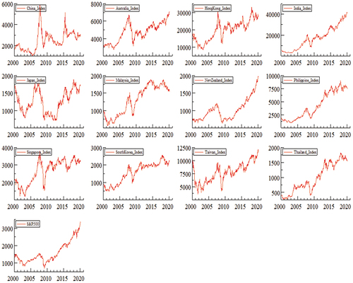
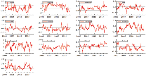
Figure 2 exhibits weekly price movements for the entire sample, weekly index returns are calculated by taking the first difference logarithms of two subsequent index prices as; rt, t = (Pi, t/Pi, t −1) × 100, where ri, t represents constantly magnified proportion rates of return for index i at time t, and Pi, t represents the index price level i at time t.

Figure 2. Exhibits weekly price movements for the entire sample.

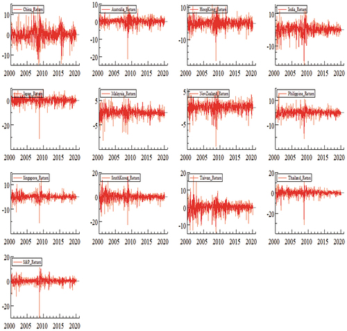
Table 1 presents the descriptive statistics of the weekly return series for all price indexes. India is the highest average (0.196%), followed by the Philippines (0.136%), while the only market with a negative return is Japan. The riskiest markets are China (3,2991%) and South Korea (3,299%), while New Zealand has the minimum risky market of (1,5643%). There is a negative skewness in the return distribution of all countries. Kurtosis results indicate that all stock market returns are leptokurtic, presenting a fat-tailed distribution supported by Jarque—Bera test in rejecting the normality of all stock market returns. Expect Japan, for all stock market returns, the hypothesis of no ARCH impacts and zero serial correlation is rejected. Finally, the return series for all stock markets are founded stationary based KPSS and ADF tests.

Table 1. Descriptive statistics of all stock markets using weekly return data

Variable	China	Australia	Hong Kong	India	Japan	Malaysia	New Zealand	Philippine	Singapore	South Korea	Taiwan	Thailand	US.
#obs	1006	1006	1006	1006	1006	1006	1006	1006	1006	1006	1006	1006	1006
min	−14.89	−21.37	−23.31	−21.87	−31.12	−11.44	−12.08	−21.35	−21.32	−22.92	−14.47	−31.44	−29.93
mean	0.0551	0.0819	0.0510	0.1968	−0.0003	0.0415	0.0979	0.1360	0.0386	0.0926	0.0154	0.1314	0.0915
max	13.94	9.11	11.71	13.17	9.24	6.65	5.34	15.44	15.32	17.03	18.31	10.75	11.35
std.dev	3.29	2.10	3.03	3.07	2.82	1.84	1.56	2.83	2.54	3.29	2.98	2.87	2.49
Skewness	−0.22	−1.40	−0.47	−0.79	−1.55	−0.61	−1.01	−0.36	−0.69	−0.62	−0.39	−1.78	−1.95
Excess Kurtosis	2.41	11.80	4.65	4.89	14.71	3.80	5.51	5.71	8.94	5.97	3.90	16.26	22.42
J-B	252.86	6172.4	947.15	1109.6	9478.1	668.22	1447.2	1393.3	3437.8	1563.6	665.83	11,627	21,730
ARCH-LM(10)	12.78	8.31	10.66	12.85	1.29	6.20	6.14	5.41	17.62	18.90	8.58	3.06	3.86
Q2(20)	393.61	150.70	233.12	255.28	16.87	178.72	122.07	93.68	260.95	452.60	273.15	44.78	69.19
ADF	−16.22	−19.38	−18.02	−17.54	−18.72	−17.35	−17.39	−17.20	−18.38	−18.78	−17.48	−17.33	−19.56
KPSS	0.0692	0.0554	0.0652	0.1068	0.2490	0.1680	0.3439	0.1409	0.0632	0.0625	0.2138	0.0724	0.2997

This research identifies a suitable ARMA-GARCH model based on the lower values of Akaike and Schwarz criteria with a lag selection of p =1, 2 and q = 1, 2 lags and found that the more appropriate one for all combination returns is ARMA (1, 1)-GARCH (1, 1). Specifically, the best-fit model is univariate ARME(1,1)-GARCH(1,1) for Australia, China, Hong Kong, India, Malaysia, New Zealand, and South Korea, whereas the best-fit model for Taiwan is ARMA(1,1)-GARCH(1,2), the best-fit model for Japan and US stock markets is ARMA(1,1)-GARCH(2,1), and lastly, ARMA(1,1)-GARCH(1,1) the best model for Philippines and Singapore.

Multivariate GARCH models that are linear in squares and cross-products of returns are typically used to estimate time-varying correlations. Engle proposes a new category of multivariate models termed dynamic conditional correlation (DCC) models (2002). It combines the adaptability of univariate GARCH models with correlation models that minimize the number of parameters. It is linear, but it can calculate simply using univariate or two-step likelihood-based approaches. Moreover, it demonstrates that it operates well in various settings and produces empirically sound outcomes.

The dynamic equicorrelation model (DECO) introduced by Engle and Kelly (2012) is a particular case of the Constant Conditional Correlation (CCC) and Dynamic Conditional Correlation (DCC) models, which include first controlling for individual volatility and then estimating correlations. A quasi-maximum likelihood estimator (QMLE) demonstrates that when the equicorrelation assumption is violated, DECO may still provide consistent parameter estimates. These models, which parameterize the conditional correlations directly, are naturally calculated in two steps; the first step is to estimate univariate GARCH models and conditional variances for each asset return series. In the second stage, the DECO model is estimated.

Table 2 shows significant terms for ARCH and GARCH, with the sum of the terms ARCH and GARCH close to the point of unity. The variance of all returns demonstrates strong persistence in the univariate GARCH model. The DECO model result is 0.2405, indicating that the dynamic equicorrelation is positive, showing that all stock markets are well integrated. The calculated DCC factors aDECO across all stock markets is 0.0187 positive and significant, which is why market shocks affect equicorrelations. The DCC factors bDECO is simultaneously significant across all markets 0,9808 and nearly is one unit, showing equicorrelationships strongly dependent on previous correlations. The importance of the factors of aDECO and bDECO, taken together, explains the suitability of the DECO-GARCH model.

Table 2. Presents the calculated result of the ARMA (1, 1)-DECO-GARCH (1, 1) model

		China		Australia	Hong Kong	India		Japan	Malaysia	New Zealand	Philippine	Singapore	South Korea	Taiwan	Thailand	US
Cst.(M)		0.0287		0.1525***	0.1557*	0.2429***		0.1394	0.0653	0.1642***	0.1919**	0.1440**	0.1080	0.1176	0.1168	0.2498***
		(0.0994)		(0.0463)	(0.0821)	(0.0864)		(0.1058)	(0.0490)	(0.0459)	(0.0828)	(0.065354)	(0.0706)	(0.0735)	(0.0843)	(0.0357)
AR(1)		0.5515***		0.7549**	−0.9174***	0.1038		−0.1094	−0.1464	0.5624*	−0.7691***	0.0121	−0.7656***	−0.9173***	0.3584	0.8970***
		(0.1859)		(0.2938)	(0.0737)	(0.2394)		(0.3423)	(0.5454)	(0.2903)	(0.0971)	(0.1435)	(0.1017)	(0.0418)	(0.2382)	(0.0498)
MA(1)		−0.4853**		−0.7982***	0.8990***	−0.0279		0.1465	0.2010	−0.5401*	0.7168***	0.0674	0.7235***	0.8845***	−0.3257	−0.9586***
		(0.1881)		(0.2727)	(0.0787)	(0.2402)		(0.3718)	(0.5348)	(0.2979)	(0.1055)	(0.1450)	(0.1113)	(0.0518)	(0.2368)	(0.0263)
Cst. (V)		0.3040		0.0674	0.1743	0.0426		0.5258*	0.0310*	0.0513	0.1385	0.1110	0.1935	0.1336**	0.0400	0.3830**
		(0.1984)		(0.0700)	(0.1118)	(0.0456)		(0.2699)	(0.0169)	(0.0450)	(0.2001)	(0.0962)	(0.1257)	(0.0645)	(0.0453)	(0.1556)
ARCH		0.1263***		0.0856**	0.0786***	0.0589***		0.1360*	0.0839***	0.0665*	0.0838	0.1390*	0.1304**	0.0944***	0.0841*	0.3708**
		(0.0456)		(0.0424)	(0.0255)	(0.0205)		(0.0752)	(0.0210)	(0.0370)	(0.0719)	(0.0733)	(0.0451)	(0.0235)	(0.0479)	(0.1743)
GARCH		0.8490***		0.9029***	0.9027***	0.9367***		0.8138***	0.9091***	0.9125***	0.9017***	0.8524***	0.8549***	0.8916***	0.9192***	0.6404***
		(0.0539)		(0.0504)	(0.0308)	(0.0230)		(0.0432)	(0.0194)	(0.0500)	(0.0873)	(0.0733)	(0.0493)	(0.0236)	(0.0378)	(0.1054)
Calculations of the DECO model
Average	0.2405*** (0.068)
adeco	0.0187*** (0.0054)
bdeco	0.9808*** (0.0058)

Diagnostic tests in Table 3 reveal that the DECO-GARCH model contains no misspecification. The Ljung Box test indicates that most stock markets lack serial correlation (excluding standard residuals of Thailand and the US). Figure 3 demonstrates the dynamic equicorrelation between all the stock markets. Over the sample timeframe, time-specific correlations are detected, which also alter the portfolio composition of the investors. Most significantly, attributable to the 2007–2009 Global Financial Crises (GFC), a significant increase in equicorrelation is identified. That suggests all returns from stock markets are becoming more interconnected increasingly, reinforcing the theory of recoupling (contagion effects). The rising contagion levels allow the instability shock to spread significantly to other stock market prices in specific stock markets. In periods of uncertainty, reducing the value of foreign investment portfolio diversification, this impact can also be seen in particular. Sensoy et al. (2015) have demonstrated that the outlook for metals in precious and consumer products has converged since the mid-2000s.

Figure 3. Dynamic equicorrelation across all stock markets.

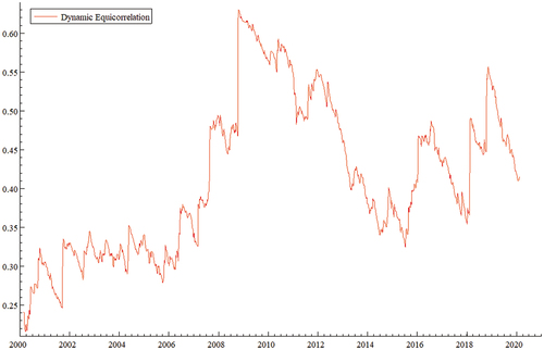
Table 3. Diagnostic tests

Akaike	53.3579
Schwartz	53.7584
Q(20)	21.1049	17.0650	26.0697	13.4878	16.1692	12.5047	20.7691	12.0373	19.8375	25.4339	16.5630	41.9797	66.6845
	(0.3910)	(0.6488)	(0.1635)	(0.8555)	(0.7061)	(0.8976)	(0.4108)	(0.9148)	(0.4681)	(0.1853)	(0.6811)	(0.0029)	(0.0000)
Q(20)	19.2063	12.0692	24.2534	29.0378	7.1895	16.4739	11.6751	17.5749	17.5737	15.2049	12.3350	16.9375	16.4696
	(0.5085)	(0.9137)	(0.2315)	(0.0870)	(0.9960)	(0.6868)	(0.9268)	(0.6154)	(0.6155)	(0.7646)	(0.9041)	(0.6570)	(0.6871)
Hosking^2 (20)	3721.39
	(0.0000)
McLeod-Li^2(20)	3719.8
	(0.0000)

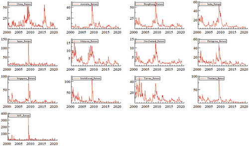
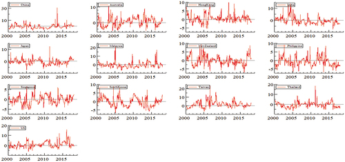
The parameter variances predicted by the DECO-GARCH model for all stock markets display in Figure 4. As in Figure 3, all conditional variances most likely have a similar movement and sequence. In high periods of volatility connected with the GFC’s potential economic development, consumer demand, and output, the conditional variances sequence is more unpredictable. The event may increase the propagation of uncertainty through such markets.

Figure 4. Conditional variances for each stock market using ARMA(1,1)- DECO-GARCH(1,1) model.

4.1. Return and volatility spillover index

Table 4 presents the total return and conditional volatility spillover index, all findings based on order one vector autoregressions and generalized 10-week forecast error variance decompositions. The average complete measure of loss for all capital markets and split it down through forward-looking transmitters (called “to others”) and the recipient (called “from others”) of uncertainty and returns are estimated. The row “Net” shows the total number of net-pair directional spillovers as positive and negative values (net-recipient).

Table 4. Dynamic Connectedness Return spillovers across all sample stock markets

	China	Australia	Hong Kong	India	Japan	Malaysia	New Zealand	Philippine	Singapore	South Korea	Taiwan	Thailand	US	FROM
China	34.78	5.30	8.60	4.35	4.52	5.71	4.03	4.47	5.89	5.92	6.03	4.81	5.53	65.21
Australia	3.72	20.94	7.73	6.07	7.54	4.49	6.75	4.80	8.36	7.85	5.95	5.44	10.27	79.05
Hong Kong	5.07	7.32	18.96	6.76	6.18	6.08	4.16	5.42	10.14	8.86	8.25	5.53	7.22	81.03
India	2.95	7.11	9.11	22.68	6.52	4.62	4.48	6.08	8.56	7.51	7.10	6.08	7.16	77.31
Japan	3.80	8.56	7.34	6.01	23.07	4.40	5.24	4.73	7.93	8.60	6.79	5.28	8.19	76.92
Malaysia	4.08	5.42	8.00	5.32	4.80	26.50	4.34	5.97	8.7	7.01	7.92	6.89	4.99	73.49
New Zealand	4.12	10.09	5.98	5.52	6.51	4.91	26.6	5.42	6.72	5.50	5.95	4.78	7.85	73.4
Philippine	3.91	6.17	7.14	6.50	4.89	6.01	4.83	25.44	8.49	7.14	6.53	7.39	5.51	74.55
Singapore	3.29	8.10	10.08	6.95	6.51	6.17	4.86	5.77	18.41	8.08	7.99	6.07	7.67	81.58
South Korea	4.34	7.83	9.24	5.98	7.20	5.23	4.22	5.17	8.11	19.86	9.8	5.20	7.77	80.13
Taiwan	3.95	6.58	8.99	6.36	5.92	6.05	4.81	5.28	8.68	10.29	20.63	5.17	7.24	79.36
Thailand	4.33	6.20	7.25	6.6	5.68	6.77	3.71	6.88	7.82	6.50	6.55	25.75	5.91	74.24
US	3.93	10.13	7.94	6.35	7.46	4.19	5.03	4.44	7.92	8.51	6.64	5.09	22.31	77.69
Contribution TO others	47.54	88.84	97.47	72.81	73.77	64.69	56.51	64.49	97.36	91.81	85.56	67.76	85.36	994.02
Contribution including own	82.33	109.79	116.43	95.49	96.84	91.19	83.11	89.94	115.78	111.67	106.19	93.51	107.67	76%
Net spillovers	−17.67	9.79	16.43	−4.50	−3.15	−8.80	−16.88	−10.05	15.78	11.67	6.19	−6.48	7.67	76.46

The cumulative returns spillover graph, as seen in Table 4, shows the average returns spillover impact is 76.46%. Hong Kong and Singapore are the major contributors (97,473%, and 97,368%, respectively) to the other stock markets in spatial spillovers distributed “to everyone”. China is nevertheless the lowest (47,546%) delegate. Regarding “other” spatial spillover, Singapore is the highest beneficiary (81.586%) to return spillover to other stock markets. Hong Kong is the most significant net transmitter of return spillovers, led by Singapore (16,434%, and 15,7837%, respectively), and China is the highest net recipient of return spillovers (−17,67%).

Table 5 displays all reference stock markets with spillover matrices with conditional volatility. The gross volatility spillover rate is 79,151 points. Taiwan is the main volatility transmitter in other markets. Taiwan is increasing its extreme positional uncertainty to 101,156%, and, on the other hand, all stock markets are moving only 78,482%. The US stock market’s second biggest total transmitter, with a net effect of 10.45%. While in these markets, the Philippines is the leading net recipient, followed by China (−11,497%, −7,298%, respectively)

Table 5. Dynamic Connectedness conditional variance volatility spillovers across all sample stock markets

	China	Australia	Hong Kong	India	Japan	Malaysia	New Zealand	Philippine	Singapore	South Korea	Taiwan	Thailand	US	FROM
China	28.23	6.71	6.38	5.88	6.01	5.73	6.28	6.47	4.56	4.91	6.56	5.86	6.35	71.76
Australia	6.31	18.16	7.73	6.28	6.38	5.01	6.42	4.64	7.45	6.69	8.56	6.43	9.88	81.83
Hong Kong	5.39	8.19	19.19	5.87	6.57	5.45	5.06	4.66	7.65	7.83	10.36	5.14	8.59	80.81
India	4.84	7.75	8.58	19.7	5.71	7.1	7.84	5.09	7.73	5.33	7.71	5.21	7.34	80.29
Japan	5.15	7.26	6.39	6.41	21.63	5.34	6.72	4.91	6.51	8.22	8.73	4.78	7.87	78.369
Malaysia	5.23	6.29	7.04	7.34	4.57	22.66	6	6.21	7.55	5.88	8.2	6.72	6.26	77.33
New Zealand	5.1	8.62	6.72	6	5.81	5.66	21.22	5.22	6.26	6.09	9.11	6.49	7.64	78.77
Philippine	5.25	5.79	7.43	5.61	5.45	8	6.21	21.13	6.84	7.54	7.64	6.81	6.25	78.86
Singapore	5.6	7.94	8.21	6.96	6.41	6.81	6.66	6.36	15.17	7.05	8.94	6.57	7.26	84.82
South Korea	5.32	7.2	8.04	5.58	8.01	5.37	6.37	5.4	6.75	17	11.35	5.81	7.73	82.99
Taiwan	5.1	7.95	7.52	5.9	5.98	5.01	6.58	5.75	7.26	8.66	21.51	5.05	7.67	78.48
Thailand	5.14	6.1	6.54	6.65	4.65	8.15	7.25	7.58	6.95	5.36	6.54	23.45	5.6	76.55
US	5.98	9.02	7.48	6.57	6.16	5.64	6.39	5.02	6.54	6.15	7.39	5.65	21.95	78.04
Contribution TO others	64.47	88.87	88.11	75.1	71.76	73.3	77.84	67.36	82.11	79.75	101.15	70.57	88.49	1028.96
Contribution including own	92.7	107.03	107.3	94.8	93.39	95.96	99.06	88.5	97.28	96.78	122.67	94.02	110.45	79%
Net spillovers	−7.29	7.03	7.3	−5.19	−6.6	−4.03	−0.93	−11.49	−2.71	−3.21	22.67	−5.97	10.45	79.15

This finding reinforced the general understanding in the global investment management group of the leading position of the countries in Asia and Pacific for investors in the worldwide equity market based on the effects of the return on and uncertainty spillovers in Tables 4 and 5.

4.2. Directional spillover effects

A main drawback of the dynamic spillover index is that there are consistent linkages between stock markets over time, as shown in previous Tables 4 and 5.

The dynamic spillover index could ignore the price and volatility changes usually caused by different crises around the world, such as the crises occurs over our sample period (2000–2020) (including the dot-com bubble in the US (2000–2002), the 2007–2009 Global financial crisis (GFC), the 2010–2012 EU sovereign debt crisis (EDC), and the 2015–2016 Chinese stock market crisis (CSMC))

These financial events happened during the sample period and impacted the direction or magnitude of the dependent on all capital markets. p Cyclical shifts and spillovers that the standard spillover index can not detect in previous Tables 4 and 5 will also be taken into account.

Figure 5 displays period fluctuations and spillovers of variability derived from 104-week; tests from rotating windows (two years) utilizing the Diebold and Yilmaz (2012). Return and volatility indexes have exhibited pretty similar cyclical trends and time-consuming blasts. Such cyclical trends and spillovers are related to many periods of financial crises, such as Dot-com bubbling, GFC, EDC, and CSMC. These three financial crises might strengthen the impact on the Asia Pacific and the US stock market’s returns and volatility spillover.

Figure 5. Dynamic total connectedness return and conditional variance volatility for all stock markets.

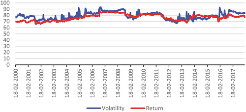
Figure 5 displays; the first phase of the Dot-com bubble started in 2000 and finished by the end of 2002. In July 2005, the aggregate spillover level began to increase once more, and regarding return and volatility spillovers, there was a significant decrease after the GFC eventually hit 76% by July 2009. For both return and volatility spillovers, there were consistently significant spillovers during the 2010–2012 EDC, although the return and volatility spillovers began to decline dramatically after April 2011. Moreover, the spillover index fell to 67% by the end of 2008, whereas the highest level of return was 84%, and volatility achieved 90% in the same year. By July 2013, spillover index returns rose to 79%, and volatility rose to 84%. Last, the lowest point of CSMC return was 69% by December 2015, while the peak level of volatility was approximately 92%. Such results are compatible with the literature’s hypothesis that market contagion is substantially growing, despite a recession shock in one sector (Forbes & Rigobon, 2002).

4.3. Net volatility spillovers

This research explored net volatility spillovers measured at the conditional volatility index, dynamic net returns, and volatility spillovers, based on 104 weeks rolling windows, to investigate further the dynamic behavior of volatility overflows. Dynamic net return and spillover rates have been determined by eliminating directional “to” spillovers from directional spillovers “from” spillovers. A sender (recipient) to (from) other financial markets implies positive (negative) values.

Figure 6a shows net return spillovers throughout the sample period over each stock market. According to the results in Table 4, the return spillover of the Hong Kong and Singapore markets significantly contributed to the other stock markets. The second highest source was Singapore’s net market return contribution of about 121% during that period, which peaked at 277% in October 2001. However, Hong Kong’s average net participation was 126% during that period, with the highest at 489% in February 2006.

Figure 6a. A Net return Spillovers.

Figure 6b indicates that the Taiwan stock market has been the most significant net volatility spillover transmitter with more than a 174%, reaching its highest amount of 2,3492% in August 2006, while its lowest value was also in January 2005 (−665%). On the other hand, in February 2016, the second highest volatility net transmitter, through a mean of 803 %, was in the US at its peak in August 2005 (−626 %).

Figure 6b. Net volatility spillovers.

Conversely, the root or receiver of both the net return and volatility spillovers is hard to identify since there is a negative or positive impact on the net spillovers, and their significance levels may have shifted during the time. In line with the Table 5 findings, Dynamic Connectedness conditional variance volatility spillovers found that the Philippines is the lowest contributor to other markets (including their markets (88.503)). At the same time, it received from the other markets (78.866), resulting in the allocated Philippines as the largest net recipients markets of volatility spillovers (−11.497) among all markets, followed by China net recipients of volatility spillovers (−7.298). On the other hand, Taiwan contributes the highest to other markets, including its market (122.675). In contrast, it received from other markets (78.482). As a result, it reached a net spillover of (22.675) to other markets, followed by the US contributing to other markets, including their market (110.45) and receiving from other markets (78.049), reaching a net spillover of (10.45).

Examine the Dynamic Connectedness Return spillovers across all sample stock markets in Table 4. Hong Kong and Singapore show a clear direction of a return to other stock marks in the sample (transmitter). In contrast, China shows a clear net recipient. However, asymmetric negative (net recipient) and positive (transmitter) values have been identified in every stock market for the volatility spillover throughout the sample period. Moreover, none in the financial markets revealed that their various macroeconomic strategies have regularly influenced volatility spillover (Click & Plummer, 2005; Majid et al., 2008).

4.4. Hedge ratios and portfolio weights

Diversification is a long-term investment strategy that entails investing in various assets to lessen the risk of volatility. Nonetheless, variation in investment portfolio is not entirely dictated by the number of holdings. For example, investors may seek to diversify beyond the primary asset classes of stocks, bonds, and cash equivalents such as certificates of deposit (CDs) and money market funds. However, diversification cannot mitigate the overall economy’s systemic investment risks.

To achieve diversification, investors must do one of the following:

• Asset diversification: a combination of equities, bonds, cash equivalents, and potentially alternative assets.

• Sector diversification entails investments in numerous stock market sectors.

• Geographic diversification: domestic and global investments.

• Time diversity, or temporal diversification, is a combination of assets that provides varied results over an extended time horizon.

However, there is a risk associated with excessive diversity. Over-diversification occurs when investors disperse their capital across so many diverse investments that portfolio returns diminish without sufficient risk reduction. Excessive diversification may make it challenging to track investments and tempt individuals to invest in stocks they do not fully know. Additionally, it can result in more significant fees, specifically if the portfolio is managed by a professional.

Investing in overlapping assets is a typical example of over-diversification. Suppose, for instance, one investor owns an S&P 500 index fund. He wishes to diversify his portfolio beyond the S&P 500, so he invests in a so-called total stock market fund to get exposure to the entire U.S. stock market. However, S&P 500 stocks represent around 80% of the market value of the U.S. stock market, so holding both would not significantly increase diversity.

No magic formula exists for determining the optimal level of variation. Even if investors buy hundreds of stocks, their portfolio is not sufficiently diversified if it focuses on only one or two industries. Benjamin Graham, the founder of value investing and Warren Buffett’s mentor, recommended holding at least 40 stocks. However, current recommendations vary depending on the proportion of particular stocks in a portfolio, as diversification may now be achieved through mutual funds and ETFs. On average, no single investment should comprise more than 5% of a portfolio. Alternatively, it might diversify by holding only three funds: one that invests in the entire U.S. stock market, one that invests in the foreign stock market, and one that invests in the total bond market (Hagstrom, 2013).

Due to its benefits, hedging is a financial technique that investors should comprehend and employ. As an investment, it safeguards an investor’s funds from exposure to a difficult circumstance that could result in a loss of value (Hwang & Satchell, 2010). However, hedging does not guarantee that investments will not decline in value. If this occurs, the losses will be offset by gains from another investment.

Hedging means identifying the risks associated with every investment and protecting from any unfavorable outcome. A derivative or contract whose value is measured by an underlying asset is a typical type of hedging. For example, consider the case of an investor who purchases shares of a company in the hopes that its price will rise. In contrast, the price falls, resulting in a loss for the investment. Such occurrences can be reduced if the investor utilizes an option to ensure that the impact of such an adverse occurrence will be offset. An option is a contract allowing the investor to buy or sell a stock at a predetermined price and time. In this situation, a put option would permit the investor to profit from the stock’s price decrease. This profit would at least partially offset his loss from purchasing the stock. That is regarded as one of the most efficient hedging tactics. (Arif et al., 2022).

Numerous studies have consistently demonstrated that different assets, such as gold, bonds, and currencies, have been successfully deployed as effective hedging assets (Arif et al., 2022; Urquhart & Zhang, 2019). In this section, we analyze whether the S&P 500 and 12 Asian stock markets represent an appropriate hedge, considering the inherent capabilities of geographic diversification.

As a consequence of the results mentioned in the previous part above, for the diversification and risk management of global portfolios, a portfolio of different markets is designed to mitigate risk without reducing anticipated returns. Assuming that an investor holds an index stock market and needs to hedge her position against unfavorable effects with another index market j. In particular, the considering of holdings on differential index markets in portfolio weight is described by Kroner and Ng (1998);

(18) ${\sum }_t^c=\frac{h_t^i-h_t^{i,j}}{h_t^i-2h_t^{i,j}+h_t^j},when{W}_t^c=\left\{\begin{array}{c}0W_t^c<0\\ W_t^{c}0\le W_t^c\le 1\\ 1W_t^C>1\end{array}\right\}$(18)

Here $h_t^i,h_t^{i,j},h_t^j$ are still the conditional variances of its i index returns, its j index return, and the conditional covariance at period t. That stock index’s optimal level is equivalent to $(1-W_t^c)$. Across each stock-index return set, the DECO-GARCH model obtains all data required to determine the value $W_t^c$.

Beta Hedge techniques were employed to reduce the risk of the whole portfolio stock market index, implemented by Krooner and Sultan (1993). How much is a short position (selling) ${\beta }_t^c$ the dollar that needs to be held in the other stock index for the long position (purchasing) of one dollar in one stock market is calculated as:

(19) ${\beta }_t^c=\frac{h_t^{i,j}}{h_t^j}$(19)

Ku et al. (2007) indicated that hedging errors could use to assess the Hedging effectiveness of the developed portfolios as computed below

(20) $HE=1-\frac{Va{r}_{hedged}}{Va{r}_{unhedged}}$(20)

In which the hedge portfolio variance ($Va{r}_{hedged}$) of two different stock market indexes, i and j are the sum of the weighted portfolio returns, the variance in the unhedged portfolio ($Va{r}_{unhedged}$) is that of the stock market index j’s returns.

Table 6 displays the outcomes of hedging effectiveness for the optimal hedge ratio strategy, while the hedging effectiveness of the optimal portfolio weights strategy is present in table 7. The average ideal weight coefficients ($W_t^c$) of each stock price index, and the average ideal hedge ratios (${\beta }_t^c$) and the hedging performance (HE).

Table 6. Performance of optimal portfolios’ hedge ratios

	${\mathit{W}}_t^c$	HE		${\mathit{W}}_t^c$	HE		${\mathit{W}}_t^c$	HE		${\mathit{W}}_t^c$	HE
China/Australia	0.37	0.55	Australia/China	0.63	0.26	Hong Kong/China	0.73	0.16	India/China	0.81	0.18
China/Hong Kong	0.27	0.63	Australia/Hong Kong	0.33	0.35	Hong Kong/Australia	0.67	0.13	India/Australia	0.83	0.09
China/India	0.19	0.76	Australia/India	0.17	0.55	Hong Kong/India	0.25	0.44	India/Hong Kong	0.75	0.15
China/Japan	0.57	0.37	Australia/Japan	0.83	0.05	Hong Kong/Japan	0.91	0.02	India/Japan	0.94	0.03
China/Malaysia	0.34	0.59	Australia/Malaysia	0.45	0.37	Hong Kong/Malaysia	0.56	0.28	India/Malaysia	0.74	0.18
China/New Zealand	0.25	0.69	Australia/New Zealand	0.3	0.42	Hong Kong/New Zealand	0.43	0.35	India/New Zealand	0.63	0.26
China/Philippine	0.29	0.55	Australia/Philippine	0.42	0.35	Hong Kong/Philippine	0.54	0.26	India/Philippine	0.71	0.2
China/Singapore	0.57	0.32	Australia/Singapore	0.83	0.03	Hong Kong/Singapore	0.96	0	India/Singapore	1	0
China/South Korea	0.53	0.39	Australia/South Korea	0.75	0.07	Hong Kong/South Korea	0.9	0.01	India/South Korea	0.93	0.03
China/Taiwan	0.4	0.52	Australia/Taiwan	0.53	0.24	Hong Kong/Taiwan	0.67	0.13	India/Taiwan	0.79	0.15
China/Thailand	0.35	0.57	Australia/Thailand	0.46	0.29	Hong Kong/Thailand	0.59	0.19	India/Thailand	0.79	0.08
China/US.	0.87	0.1	Australia/U.S.	1	0	Hong Kong/U.S.	1	0	India/ US.	1	0
Japan/China	0.43	0.47	Malaysia/China	0.66	0.29	New Zealand/China	0.75	0.19	Philippine/China	0.71	0.21
Japan/Australia	0.17	0.51	Malaysia/Australia	0.55	0.34	New Zealand/Australia	0.7	0.1	Philippine/Australia	0.58	0.32
Japan/Hong Kong	0.09	0.63	Malaysia/Hong Kong	0.44	0.44	New Zealand/Hong Kong	0.57	0.25	Philippine/Hong Kong	0.46	0.42
Japan/India	0.06	0.76	Malaysia/India	0.26	0.58	New Zealand/India	0.37	0.44	Philippine/India	0.29	0.59
Japan/Malaysia	0.25	0.6	Malaysia/Japan	0.75	0.18	New Zealand/Japan	0.86	0	Philippine/Japan	0.78	0.15
Japan/New Zealand	0.14	0.67	Malaysia/New Zealand	0.39	0.51	New Zealand/Malaysia	0.61	0.27	Philippine/Malaysia	0.52	0.36
Japan/Philippine	0.22	0.59	Malaysia/Philippine	0.48	0.35	New Zealand/Philippine	0.59	0.21	Philippine/New Zealand	0.41	0.47
Japan/Singapore	0.5	0.24	Malaysia/Singapore	0.79	0.1	New Zealand/Singapore	0.86	0.01	Philippine/Singapore	0.8	0.1
Japan/South Korea	0.44	0.27	Malaysia/South Korea	0.73	0.16	New Zealand/South Korea	0.82	0.04	Philippine/South Korea	0.75	0.16
Japan/Taiwan	0.27	0.49	Malaysia/Taiwan	0.58	0.32	New Zealand/Taiwan	0.7	0.17	Philippine/Taiwan	0.6	0.29
Japan/Thailand	0.24	0.55	Malaysia/Thailand	0.52	0.33	New Zealand/Thailand	0.62	0.2	Philippine/Thailand	0.54	0.31
Japan/ US.	0.92	0.02	Malaysia/US.	0.94	0.03	New Zealand/US.	0.98	−0.02	Philippine/US.	0.98	0
Singapore/China	0.43	0.48	South Korea/China	0.47	0.46	Taiwan/China	0.6	0.32	Thailand/China	0.65	0.32
Singapore/Australia	0.17	0.55	South Korea/Australia	0.25	0.51	Taiwan/Australia	0.47	0.35	Thailand/Australia	0.54	0.33
Singapore/Hong Kong	0.04	0.66	South Korea/Hong Kong	0.1	0.61	Taiwan/Hong Kong	0.33	0.45	Thailand/Hong Kong	0.41	0.43
Singapore/India	0	0.77	South Korea/India	0.07	0.75	Taiwan/India	0.21	0.65	Thailand/India	0.21	0.57
Singapore/Japan	0.5	0.31	South Korea/Japan	0.56	0.24	Taiwan/Japan	0.73	0.16	Thailand/Japan	0.76	0.16
Singapore/Malaysia	0.21	0.6	South Korea/Malaysia	0.27	0.58	Taiwan/Malaysia	0.42	0.45	Thailand/Malaysia	0.48	0.39
Singapore/New Zealand	0.14	0.71	South Korea/New Zealand	0.18	0.67	Taiwan/New Zealand	0.3	0.55	Thailand/New Zealand	0.38	0.52
Singapore/Philippine	0.2	0.6	South Korea/Philippine	0.25	0.58	Taiwan/Philippine	0.4	0.43	Thailand/Philippine	0.46	0.38
Singapore/South Korea	0.44	0.29	South Korea/Singapore	0.56	0.19	Taiwan/Singapore	0.75	0.1	Thailand/Singapore	0.8	0.09
Singapore/Taiwan	0.25	0.51	South Korea/Taiwan	0.25	0.42	Taiwan/South Korea	0.75	0.07	Thailand/South Korea	0.75	0.13
Singapore/Thailand	0.2	0.55	South Korea/Thailand	0.25	0.51	Taiwan/Thailand	0.43	0.39	Thailand/Taiwan	0.57	0.32
Singapore/US.	0.91	0.04	South Korea/US.	0.92	0.02	Taiwan/US.	0.95	0.02	Thailand/US.	0.96	0.02
US./China	0.13	0.83
US./Australia	0	0.89
US./Hong Kong	0	0.92
US./India	0	0.94
US./Japan	0.08	0.78
US./Malaysia	0.06	0.89
US./New Zealand	0.02	0.93
US./Philippine	0.02	0.89
US./Singapore	0.09	0.76
US./South Korea	0.08	0.79
US./Taiwan	0.05	0.87
US./Thailand	0.04	0.88

*the optimal hedge ratio strategy should not be preferred

Table 7. Performance optimal portfolios’ weights

	${\mathit{\beta }}_t^c$		HE			${\mathit{\beta }}_t^c$		HE		${\mathit{\beta }}_t^c$	HE		${\mathit{\beta }}_t^c$	HE
China/Australia	0.37		0.55	Australia/China		0.63		0.26	Hong Kong/China	0.73	0.16	India/China	0.81	0.18
China/Hong Kong	0.27		0.63	Australia/Hong Kong		0.33		0.35	Hong Kong/Australia	0.67	0.13	India/Australia	0.83	0.09
China/India	0.19		0.76	Australia/India		0.17		0.55	Hong Kong/India	0.25	0.44	India/Hong Kong	0.75	0.15
China/Japan	0.57		0.37	Australia/Japan		0.83		0.05	Hong Kong/Japan	0.91	0.02	India/Japan	0.94	0.03
China/Malaysia	0.34		0.59	Australia/Malaysia		0.45		0.37	Hong Kong/Malaysia	0.56	0.28	India/Malaysia	0.74	0.18
China/New Zealand	0.25		0.69	Australia/New Zealand		0.3		0.42	Hong Kong/New Zealand	0.43	0.35	India/New Zealand	0.63	0.26
China/Philippine	0.29		0.55	Australia/Philippine		0.42		0.35	Hong Kong/Philippine	0.54	0.26	India/Philippine	0.71	0.2
China/Singapore	0.57		0.32	Australia/Singapore		0.83		0.03	Hong Kong/Singapore	0.96	0	India/Singapore	1	0
China/South Korea	0.53		0.39	Australia/South Korea		0.75		0.07	Hong Kong/South Korea	0.9	0.01	India/South Korea	0.93	0.03
China/Taiwan	0.4		0.52	Australia/Taiwan		0.53		0.24	Hong Kong/Taiwan	0.67	0.13	India/Taiwan	0.79	0.15
China/Thailand	0.35		0.57	Australia/Thailand		0.46		0.29	Hong Kong/Thailand	0.59	0.19	India/Thailand	0.79	0.08
China/ US.	0.87		0.1	Australia/U.S.		1		0	Hong Kong/U.S.	1	0	India/ US.	1	0
Japan/China	0.43		0.47	Malaysia/China		0.66		0.29	New Zealand/China	0.75	0.19	Philippine/China	0.71	0.21
Japan/Australia	0.17		0.51	Malaysia/Australia		0.55		0.34	New Zealand/Australia	0.7	0.1	Philippine/Australia	0.58	0.32
	${\mathit{\beta }}_t^c$		HE			${\mathit{\beta }}_t^c$		HE		${\mathit{\beta }}_t^c$	HE		${\mathit{\beta }}_t^c$	HE
Japan/Hong Kong	0.09		0.63	Malaysia/Hong Kong		0.44		0.44	New Zealand/Hong Kong	0.57	0.25	Philippine/Hong Kong	0.46	0.42
Japan/India	0.06		0.76	Malaysia/India		0.26		0.58	New Zealand/India	0.37	0.44	Philippine/India	0.29	0.59
Japan/Malaysia	0.25		0.6	Malaysia/Japan		0.75		0.18	New Zealand/Japan	0.86	0	Philippine/Japan	0.78	0.15
Japan/New Zealand	0.14		0.67	Malaysia/New Zealand		0.39		0.51	New Zealand/Malaysia	0.61	0.27	Philippine/Malaysia	0.52	0.36
Japan/Philippine	0.22		0.59	Malaysia/Philippine		0.48		0.35	New Zealand/Philippine	0.59	0.21	Philippine/New Zealand	0.41	0.47
Japan/Singapore	0.5		0.24	Malaysia/Singapore		0.79		0.1	New Zealand/Singapore	0.86	0.01	Philippine/Singapore	0.8	0.1
Japan/South Korea	0.44		0.27	Malaysia/South Korea		0.73		0.16	New Zealand/South Korea	0.82	0.04	Philippine/South Korea	0.75	0.16
Japan/Taiwan	0.27		0.49	Malaysia/Taiwan		0.58		0.32	New Zealand/Taiwan	0.7	0.17	Philippine/Taiwan	0.6	0.29
Japan/Thailand	0.24		0.55	Malaysia/Thailand		0.52		0.33	New Zealand/Thailand	0.62	0.2	Philippine/Thailand	0.54	0.31
Japan/ US.	0.92		0.02	Malaysia/US.		0.94		0.03	New Zealand/US.	0.98	−0.02	Philippine/US.	0.98	0
	Mean	HE			Mean		HE			Mean	HE		Mean	HE
Singapore/China	0.43	0.48		South Korea/China	0.47		0.46		Taiwan/China	0.6	0.32	Thailand/China	0.65	0.32
Singapore/Australia	0.17	0.55		South Korea/Australia	0.25		0.51		Taiwan/Australia	0.47	0.35	Thailand/Australia	0.54	0.33
Singapore/Hong Kong	0.04	0.66		South Korea/Hong Kong	0.1		0.61		Taiwan/Hong Kong	0.33	0.45	Thailand/Hong Kong	0.41	0.43
Singapore/India	0	0.77		South Korea/India	0.07		0.75		Taiwan/India	0.21	0.65	Thailand/India	0.21	0.57
Singapore/Japan	0.5	0.31		South Korea/Japan	0.56		0.24		Taiwan/Japan	0.73	0.16	Thailand/Japan	0.76	0.16
Singapore/Malaysia	0.21	0.6		South Korea/Malaysia	0.27		0.58		Taiwan/Malaysia	0.42	0.45	Thailand/Malaysia	0.48	0.39
Singapore/New Zealand	0.14	0.71		South Korea/New Zealand	0.18		0.67		Taiwan/New Zealand	0.3	0.55	Thailand/New Zealand	0.38	0.52
Singapore/Philippine	0.2	0.6		South Korea/Philippine	0.25		0.58		Taiwan/Philippine	0.4	0.43	Thailand/Philippine	0.46	0.38
Singapore/South Korea	0.44	0.29		South Korea/Singapore	0.56		0.19		Taiwan/Singapore	0.75	0.1	Thailand/Singapore	0.8	0.09
Singapore/Taiwan	0.25	0.51		South Korea/Taiwan	0.25		0.42		Taiwan/South Korea	0.75	0.07	Thailand/South Korea	0.75	0.13
Singapore/Thailand	0.2	0.55		South Korea/Thailand	0.25		0.51		Taiwan/Thailand	0.43	0.39	Thailand/Taiwan	0.57	0.32
Singapore/US.	0.91	0.04		South Korea/US.	0.92		0.02		Taiwan/US.	0.95	0.02	Thailand/US.	0.96	0.02
	Mean	HE			Mean		HE			Mean	HE		Mean	HE
US./China	0.13	0.83
US./Australia	0	0.89
US./Hong Kong	0	0.92
US./India	0	0.94
US./Japan	0.08	0.78
US./Malaysia	0.06	0.89
US./New Zealand	0.02	0.93
US./Philippine	0.02	0.89
US./Singapore	0.09	0.76
US./South Korea	0.08	0.79
US./Taiwan	0.05	0.87
US./Thailand	0.04	0.88

*The optimal portfolio weights strategy should not be preferred.

Table 6 shows that the hedge ratio of best portfolios results from the 13-stock market index varied from 19 to 57 cents per dollar, which indicates that India (19 cents) is the cheapest $1 hedge ratio between a long and short position for China, whereas Japan (57 cents) is costly. Japan stock index is, therefore, the least effective index to hedge in contrast to China volatility. On the other hand, it is also apparent that the hedging between China and the US is ineffective and must not be chosen.

Additionally, the predicted average hedge-ratio value for; Australia is 17 to 63 cents per dollar, Hong Kong is 25 to 73 cents per dollar, India is 63 to 81 cents per dollar, Japan is 6 to 44 cents per dollar, Malaysia is 26 to 75 cents per dollar, New Zealand is 37 to 75 cents per dollar, the Philippines is 29 to 71 cents per dollar, Singapore is 4 to 50 cents per dollar, South Korea is 10 to 56 cents per dollar, Taiwan is 21 to 73 cents per dollar, Thailand is 21 to 75 cents per dollar, and the US is 2 to 13 cents per dollar.

China, Austria, Hong Kong, Japan, Malaysia, New Zealand, Philippines, Taiwan, and Thailand, the optimum hedge ratio would be beneficial on average if it hedges against India. At the same time, the optimum hedge ratio in Singapore and South Korea, would be beneficial on average if it hedges against Hong Kong. And India and the US, the optimum hedge ratio would be beneficial on average if it hedges against New Zealand.

Turning to the performance optimal portfolios’ weight in Table 7, for China, the maximum hedging effectiveness for volatility attained by hedging with India (76%), the average weight portfolio for China/India is 0.19. Every 19 cents invested in China can be hedging by 81 cent invested in India. Whereas For Australia hedging with India (55%), the average weight portfolio for Australia/India is 0.17. for Hong Kong hedging with India (44%), the average weight portfolio for Hong Kong /India is 0.25. for India hedging with New Zealand (26%), the average weight portfolio for India/New Zealand is 0.63. for Japan hedging with India (76%), the average weight portfolio for Japan /India is 0.06. for Malaysia hedging with India (58%), the average weight portfolio for Malaysia/India is 0.26. for New Zealand hedging with India (44%), the average weight portfolio for New Zealand/India is 0.37. for Philippine hedging with India (59%), the average weight portfolio for Philippine/India is 0.29. for Singapore hedging with Hong Kong (66%), the average weight portfolio for Singapore/Hong Kong is 0.04. for South Korea hedging with India (75%), the average weight portfolio for South Korea/India is 0.07. for Taiwan hedging with India (65%), the average weight portfolio for Taiwan/India is 0.21. for Thailand hedging with India (57%), the average weight portfolio for Thailand/India is 0.21. for the US the hedging with New Zealand (93 %), the average weight portfolio for US/New Zealand is 0.02.

Table 7 provides a significant increase in risk reduction to the non-hedged position, which is attributable to the optimal portfolio weights strategy. The greatest hedge-efficiency can be designed by developing a portfolio with India, particularly for China, Australia, Hong Kong, Japan, Malaysia, New Zealand, Philippines, South Korea, Taiwan, and Thailand. In comparison, India’s volatility will reach the maximum hedging efficiency by creating a portfolio with New Zealand. At the same time, the maximum hedging performance in Singapore volatility can be designed as a portfolio with Hong Kong. Finally, a portfolio in New Zealand can achieve the highest hedging effectiveness for US volatility.

5. Conclusion

This study assesses the impact of return and volatility spillover on the performance of US stock markets (S&P 500) and 12 stock markets in Asia-Pacific countries. Data covers the last two decades (from January 2000 to February 2020). The spillover index and a DECO-GARCH model are applied to weekly data to determine the usefulness of hedging stock portfolios across markets. As a result, when a more extended period and a more extensive sample data set are considered, the highest return spillover to others comes from Hong Kong and Singapore. In contrast, the highest volatility spillover to others comes from Taiwan and Australia.

The main finding of this research is that the leading stock market (S&P 500 market) does not affect the performance of other Asian-Pacific markets. Applying appropriate portfolio hedging ratios implies that international investors interested in the Asian-Pacific financial markets could not construct portfolio diversity by including the US market.

When it comes to international investors engaged in the Asian-Pacific stock markets, the most significant implication of this research is that India offers diversification investment opportunities. For example, suppose investors hedge their investments with India. In that case, the optimal hedge ratio strategy will be favored if they hedge their investments with China, Australia, Hong Kong, Japan, Malaysia, New Zealand, the Philippines, Taiwan, or Thailand. The ideal portfolio weights approach will produce more substantial benefits from risk management than hedged positions. For example, creating a portfolio with India can provide stability for China, Australia, Hong Kong, Japan, Malaysia, New Zealand, the Philippines, South Korea, Taiwan, and Thailand, among other countries. Lastly, the empirical findings demonstrate that the direction of causality in the Asian-Pacific markets differs from one country to another. Thus, this study indicates that global investors and policymakers consider country-level outcomes rather than regional outcomes.

Disclosure statement

No potential conflict of interest was reported by the author(s).

Additional information

Funding

The author received no direct funding for this research.

References

- Abdulrazzaq, Y. M., Morales, L., & Coughlan, J. (2019). Oil sector spillover effects to the Kuwait stock market in the context of uncertainty. Economics, Management & Financial Markets, 14, 1. https://www.ceeol.com/search/article-detail?id=752535
- Aboura, S., & Chevallier, J. (2014). Volatility equicorrelation: A cross-market perspective. Economics Letters, 122(2), 289–38. https://doi.org/10.1016/j.econlet.2013.12.008
- Ahmed, R. I., Zhao, G., & Habiba, U. (2022). Dynamics of return linkages and asymmetric volatility spillovers among Asian emerging stock markets. The Chinese Economy, 55(2), 156–167. https://doi.org/10.1080/10971475.2021.1930292
- Aielli, G. P. (2013). Dynamic conditional correlation: On properties and estimation. Journal of Business & Economic Statistics, 31(3), 282–299. https://doi.org/10.1080/07350015.2013.771027
- Arif, M., Naeem, M. A., Farid, S., Nepal, R., & Jamasb, T. (2022). Diversifier or more? Hedge and safe haven properties of green bonds during COVID-19. Energy Policy, 168, 113102. https://doi.org/10.1016/j.enpol.2022.113102
- Arouri, M. E. H., Jouini, J., & Nguyen, D. K. (2011). Volatility spillovers between oil prices and stock sector returns: Implications for portfolio management. Journal of International Money and Finance, 30(7), 1387–1405. https://doi.org/10.1016/j.jimonfin.2011.07.008
- Athari, S. A., & Hung, N. T. (2022). Time–frequency return co-movement among asset classes around the COVID-19 outbreak: Portfolio implications. Journal of Economics and Finance, 46(4), 736–756. https://doi.org/10.1007/s12197-022-09594-8
- Athari, S. A., Kondoz, M., & Kirikkaleli, D. (2021). Dependency between sovereign credit ratings and economic risk: Insight from Balkan countries. Journal of Economics and Business, 116, 105984. https://doi.org/10.1016/j.jeconbus.2021.105984
- Baele, L., Ferrando, A., Hördahl, P., Krylova, E., & Monnet, C. (2004). Measuring European financial integration. Oxford Review of Economic Policy, 20(4), 509–530. https://doi.org/10.1093/oxrep/grh030
- Baig, T., & Goldfajn, I. (1999). Financial market contagion in the Asian crisis. IMF Staff Papers, 46(2), 167–195. https://doi.org/10.2307/3867666
- Bala, D. A., & Takimoto, T. (2017). Stock markets volatility spillovers during financial crises: A DCC-MGARCH with skewed-t density approach. Borsa Istanbul Review, 17(1), 25–48. https://doi.org/10.1016/j.bir.2017.02.002
- Bekaert, G., & Harvey, C. R. (1995). Time‐varying world market integration. the Journal of Finance, 50(2), 403–444. https://doi.org/10.1111/j.1540-6261.1995.tb04790.x
- Bekaert, G., & Hodrick, R. J. (1992). Characterizing predictable components in excess returns on equity and foreign exchange markets. The Journal of Finance, 47(2), 467–509. https://doi.org/10.1111/j.1540-6261.1992.tb04399.x
- Bollerslev, T. (1986). Generalized autoregressive conditional heteroskedasticity. Journal of Econometrics, 31(3), 307–327.
- Bonilla, C. A., & Sepúlveda, J. (2011). Stock returns in emerging markets and the use of GARCH models. Applied Economics Letters, 18(14), 1321–1325. https://doi.org/10.1080/13504851.2010.537615
- Campbell, J. Y., & Hamao, Y. (1992). Predictable stock returns in the United States and Japan: A study of long‐term capital market integration. The Journal of Finance, 47(1), 43–69. https://doi.org/10.1111/j.1540-6261.1992.tb03978.x
- Caporale, G. M., Pittis, N., & Spagnolo, N. (2006). Volatility transmission and financial crises. Journal of Economics and Finance, 30(3), 376–390. https://doi.org/10.1007/BF02752742
- Cashin, M. P., Kumar, M. M. S., & McDermott, M. C. J. (1995). International integration of equity markets and contagion effects. International Monetary Fund.
- Chan, K. C., Fung, H. G., & Leung, W. K. (2004). Daily volatility behavior in Chinese futures markets. Journal of International Financial Markets, Institutions and Money, 14(5), 491–505. https://doi.org/10.1016/j.intfin.2004.01.002
- Chen, J., & Wang, X. (2021). Asymmetric risk spillovers between China and ASEAN Stock Markets. IEEE Access, 9, 141479–141503. https://doi.org/10.1109/ACCESS.2021.3119932
- Cheung, Y. L., Cheung, Y. W., & Ng, C. C. (2007). East Asian equity markets, financial crises, and the Japanese currency. Journal of the Japanese and International Economies, 21(1), 138–152. https://doi.org/10.1016/j.jjie.2005.11.003
- Chou, M. R. Y. T., Ng, M. V., & Pi, L. K. (1994). Cointegration of international stock market indices. International Monetary Fund.
- Christensen, B. J., & Nielsen, M. Ø. (2007). The effect of long memory in volatility on stock market fluctuations. The Review of Economics and Statistics, 89(4), 684–700. https://doi.org/10.1162/rest.89.4.684
- Clark, P. K. (1973). A subordinated stochastic process model with finite variance for speculative prices. Econometrica: Journal of the Econometric Society, 41(1), 135–155. https://doi.org/10.2307/1913889
- Click, R. W., & Plummer, M. G. (2005). Stock market integration in ASEAN after the Asian financial crisis. Journal of Asian Economics, 16(1), 5–28. https://doi.org/10.1016/j.asieco.2004.11.018
- Diebold, F. X., & Yilmaz, K. (2012). Better to give than to receive: Predictive directional measurement of volatility spillovers. International Journal of Forecasting, 28(1), 57–66. https://doi.org/10.1016/j.ijforecast.2011.02.006
- Dungey, M., Milunovich, G., & Thorp, S. (2010). Unobservable shocks as carriers of contagion. Journal of Banking & Finance, 34(5), 1008–1021. https://doi.org/10.1016/j.jbankfin.2009.11.006
- Engle, R. (2002). Dynamic conditional correlation: A simple class of multivariate generalized autoregressive conditional heteroskedasticity models. Journal of Business & Economic Statistics, 20(3), 339–350. https://doi.org/10.1198/073500102288618487
- Engle, R., & Kelly, B. (2012). Dynamic equicorrelation. Journal of Business & Economic Statistics, 30(2), 212–228. https://doi.org/10.1080/07350015.2011.652048
- Engle, R. F., Ng, V. K., & Rothschild, M. (1990). Asset pricing with a factor-ARCH covariance structure: Empirical estimates for treasury bills. Journal of Econometrics, 45(1–2), 213–237. https://doi.org/10.1016/0304-4076(90)90099-F
- Eun, C. S., & Shim, S. (1989). International transmission of stock market movements. Journal of Financial and Quantitative Analysis, 24(2), 241–256. https://doi.org/10.2307/2330774
- Favero, C. A., & Giavazzi, F. (2002). Is the international propagation of financial shocks non-linear?: Evidence from the ERM. Journal of International Economics, 57(1), 231–246. https://doi.org/10.1016/S0022-1996(01)00139-8
- Forbes, K. J., & Rigobon, R. (2002). No contagion, only interdependence: Measuring stock market co-movements. The Journal of Finance, 57(5), 2223–2261. https://doi.org/10.1111/0022-1082.00494
- Fujiwara, I., & Takahashi, K. (2012). Asian financial linkage: Macro‐finance dissonance. Pacific Economic Review, 17(1), 136–159. https://doi.org/10.1111/j.1468-0106.2011.00575.x
- Gębka, B. (2012). The dynamic relation between returns, trading volume, and volatility: Lessons from spillovers between Asia and the United States. Bulletin of Economic Research, 64(1), 65–90. https://doi.org/10.1111/j.1467-8586.2010.00371.x
- Gong, X., Liu, Y., & Wang, X. (2021). Dynamic volatility spillovers across oil and natural gas futures markets based on a time-varying spillover method. International Review of Financial Analysis, 76, 101790. https://doi.org/10.1016/j.irfa.2021.101790
- Granger, C. W. J. (1986). Developments in the study of cointegrated economic variables. Oxford Bulletin of economics and statistics, 48(3), 213–228.
- Gulzar, S., Mujtaba Kayani, G., Xiaofen, H., Ayub, U., & Rafique, A. (2019). Financial cointegration and spillover effect of global financial crisis: A study of emerging Asian financial markets. Economic research-Ekonomska istraživanja, 32(1), 187–218. https://doi.org/10.1080/1331677X.2018.1550001
- Hagstrom, R. G. (2013). The Warren Buffett Way. John Wiley & Sons.
- Hamao, Y., Masulis, R. W., & Ng, V. (1990). Correlations in price changes and volatility across international stock markets. The Review of Financial Studies, 3(2), 281–307. https://doi.org/10.1093/rfs/3.2.281
- Harrison, B., & Moore, W. (2009). Stock market co-movement in the European Union and transition countries. Financial Studies, 3, 2–28. https://d1wqtxts1xzle7.cloudfront.net/8336059/vol13i3p124-151-libre.pdf?1390855067=&response-content-disposition=inline%3B+filename%3DSTOCK_MARKET_COMOVEMENT_IN_THE_EUROPEAN.pdf&Expires=1675540577&Signature=Sh42mtB6x-EaAytViyXVxfp8mrKLS3aJwL~clAYMs1e-X76Vhpo-zIYeDSaLglgCTXuXQKqqyATCZ7sIESv4HAOvCKo6-2w-TWeGl59Vn3xAcculsFG-ZTpD5sZj-HT6S2ds2Hb2-Q5YQyS6raFqXl2wLn6LqkwaWmO1LephGwJyQb6K4O-u0Jq619ZuUZLn0HF-XdB2vcVJNesBj2n9wpnr3BtAlPGlhYkbm~V52KjfVaQpoTXYPQPAxKq1T9UYa6Vb2TSeL5vGc-PlpGRcHRAlE3luY1vOEmoInol1VzpRK613tK3SPX-vUSFUXV9W7x2-5PF~KpYqQPvpC-5pxg__&Key-Pair-Id=APKAJLOHF5GGSLRBV4ZA
- Hong, D., Lee, C., & Swaminathan, B. (2003). Earnings momentum in international markets
- Hong, Y., Liu, Y., & Wang, S. (2009). Granger causality in risk and detection of extreme risk spillover between financial markets. Journal of Econometrics, 150(2), 271–287. https://doi.org/10.1016/j.jeconom.2008.12.013
- Hong, H., Torous, W., & Valkanov, R. (2002). Do Industries Lead the Stock Market? Gradual Diffusion of Information and Cross-Asset Return Predictability. Finance. Retrieved from https://escholarship.org/uc/item/6x49x543
- Hung, N. T., & Vo, X. V. (2021). Directional spillover effects and time-frequency nexus between oil, gold and stock markets: Evidence from pre and during COVID-19 outbreak. International Review of Financial Analysis, 76, 101730. https://doi.org/10.1016/j.irfa.2021.101730
- Hussain, S. I., Nur-Firyal, R., & Ruza, N. (2022). Linkage transitions between oil and the stock markets of countries with the highest COVID-19 cases. Journal of Commodity Markets, 28, 100236. https://doi.org/10.1016/j.jcomm.2021.100236
- Hwang, J. K. (2014). Spillover effects of the 2008 financial crisis in Latin America stock markets. International Advances in Economic Research, 20(3), 311–324. https://doi.org/10.1007/s11294-014-9472-1
- Hwang, S., & Satchell, S. E. (2010). How loss averse are investors in financial markets? J. Bank. Finance, 34(10), 2425–2438. https://doi.org/10.1016/j.jbankfin.2010.03.018
- Jebran, K., Chen, S., Ullah, I., & Mirza, S. S. (2017). Does volatility spillover among stock markets varies from normal to turbulent periods? Evidence from emerging markets of Asia. The Journal of Finance and Data Science, 3(1–4), 20–30. https://doi.org/10.1016/j.jfds.2017.06.001
- Kang, S. H., Uddin, G. S., Troster, V., & Yoon, S. M. (2019). Directional spillover effects between ASEAN and world stock markets. Journal of Multinational Financial Management, 52, 100592. https://doi.org/10.1016/j.mulfin.2019.100592
- Kannadas, S., & Viswanathan, T. (2022). Volatility spillover effects among gold, oil and stock markets: Empirical evidence from the g7 countries. Economic Studies, 31(4). https://www.ceeol.com/search/article-detail?id=1040745
- King, M. A., & Wadhwani, S. (1990). Transmission of volatility between stock markets. The Review of Financial Studies, 3(1), 5–33. https://doi.org/10.1093/rfs/3.1.5
- Kirikkaleli, D., & Athari, S. A. (2020). Time-frequency co-movements between bank credit supply and economic growth in an emerging market: Does the bank ownership structure matter? The North American Journal of Economics and Finance, 54, 101239. https://doi.org/10.1016/j.najef.2020.101239
- Kondoz, M., Bora, I., Kirikkaleli, D., & Athari, S. (2019). Testing the volatility spillover between crude oil price and the US stock market returns. Management Science Letters, 9(8), 1221–1230. https://doi.org/10.5267/j.msl.2019.4.019
- Kondoz, M., Kirikkaleli, D., & Athari, S. A. (2021). Time-frequency dependencies of financial and economic risks in South American countries. The Quarterly Review of Economics and Finance, 79, 170–181. https://doi.org/10.1016/j.qref.2020.05.014
- Koop, G., Pesaran, M. H., & Potter, S. M. (1996). Impulse response analysis in nonlinear multivariate models. Journal of Econometrics, 74(1), 119–147. https://doi.org/10.1016/0304-4076(95)01753-4
- Kroner, K. F., & Ng, V. K. (1998). Modeling asymmetric co-movements of asset returns. The Review of Financial Studies, 11(4), 817–844. https://doi.org/10.1093/rfs/11.4.817
- Kroner, K. F., & Sultan, J. (1993). Time-varying distributions and dynamic hedging with foreign currency futures. The Journal of Financial and Quantitative Analysis, 28(4), 535–551.
- Ku, Y. H. H., Chen, H. C., & Chen, K. H. (2007). On the application of the dynamic conditional correlation model in estimating optimal time-varying hedge ratios. Applied Economics Letters, 14(7), 503–509. https://doi.org/10.1080/13504850500447331
- Kyle, A. S. (1985). Continuous auctions and insider trading. Econometrica: Journal of the Econometric Society, 53(6), 1315–1335. https://doi.org/10.2307/1913210
- Lee, S. B., & Kim, K. J. (1993). Does the October 1987 crash strengthen the co‐movements among national stock markets? Review of Financial Economics, 3(1), 89–102. https://doi.org/10.1002/j.1873-5924.1993.tb00574.x
- Leung, H., Schiereck, D., & Schroeder, F. (2017). Volatility spillovers and determinants of contagion: Exchange rate and equity markets during crises. Economic Modelling, 61, 169–180. https://doi.org/10.1016/j.econmod.2016.12.011
- Lien, D., Lee, G., Yang, L., & Zhang, Y. (2018). Volatility spillovers among the US and Asian stock markets: A comparison between the periods of Asian currency crisis and subprime credit crisis. The North American Journal of Economics and Finance, 46, 187–201. https://doi.org/10.1016/j.najef.2018.04.006
- Liu, L. (2014). Extreme downside risk spillover from the United States and Japan to Asia-Pacific stock markets. International Review of Financial Analysis, 33, 39–48. https://doi.org/10.1016/j.irfa.2013.07.009
- Liu, T., & Gong, X. (2020). Analyzing time-varying volatility spillovers between the crude oil markets using a new method. Energy Economics, 87, 104711. https://doi.org/10.1016/j.eneco.2020.104711
- Liu, K., Luo, C., & Li, Z. (2019). Investigating the risk spillover from crude oil market to BRICS stock markets based on Copula-POT-CoVaR models. Quantitative Finance and Economics, 3(4), 754–771. https://doi.org/10.3934/QFE.2019.4.754
- Liu, Z., Tseng, H. K., Wu, J. S., & Ding, Z. (2020). Implied volatility relationships between crude oil and the US stock markets: Dynamic correlation and spillover effects. Resources Policy, 66, 101637. https://doi.org/10.1016/j.resourpol.2020.101637
- Longin, F., & Solnik, B. (1995). Is the correlation in international equity returns constant: 1960–1990? Journal of International Money and Finance, 14(1), 3–26. https://doi.org/10.1016/0261-5606(94)00001-H
- Majid, M., Meera, A., & Omar, M. (2008). Interdependence of ASEAN-5 stock markets from the US and Japan. Global Economic Review, 37(2), 201–225. https://doi.org/10.1080/12265080802021201
- Markowitz, H. (1952). The utility of wealth. Journal of Political Economy, 60(2), 151–158. https://doi.org/10.1086/257177
- Mathur, I., & Subrahmanyam, V. (1990). Interdependencies among the Nordic and US stock markets. The Scandinavian Journal of Economics, 92(4), 587–597. https://doi.org/10.2307/3440394
- Melvin, M. (2003). A stock market boom during a financial crisis?: ADRs and capital outflows in Argentina. Economics Letters, 81(1), 129–136. https://doi.org/10.1016/S0165-1765(03)00156-3
- Mensi, W., Beljid, M., Boubaker, A., & Managi, S. (2013). Correlations and volatility spillovers across commodity and stock markets: Linking energies, food, and gold. Economic Modelling, 32, 15–22. https://doi.org/10.1016/j.econmod.2013.01.023
- Mensi, W., Maitra, D., Vo, X. V., & Kang, S. H. (2021). Asymmetric volatility connectedness among main international stock markets: A high frequency analysis. Borsa Istanbul Review, 21(3), 291–306. https://doi.org/10.1016/j.bir.2020.12.003
- Milunovich, G., & Thorp, S. (2006). Valuing volatility spillovers. Global Finance Journal, 17(1), 1–22. https://doi.org/10.1016/j.gfj.2006.06.007
- Panda, A. K., & Nanda, S. (2018). Time-varying synchronization and dynamic conditional correlation among the stock market returns of leading South American economies. International Journal of Managerial Finance, 14(2), 245–262. https://doi.org/10.1108/IJMF-11–2016-0206
- Panda, P., Vasudevan, S., & Panda, B. (2021). Dynamic Connectedness among BRICS and major Countries Stock Markets. Journal of Public Affairs, 21(3), e2265. https://doi.org/10.1002/pa.2265
- Pesaran, M. H., & Pick, A. (2007). Econometric issues in the analysis of contagion. Journal of Economic Dynamics and Control, 31(4), 1245–1277. https://doi.org/10.1016/j.jedc.2006.03.008
- Pesaran, H. H., & Shin, Y. (1998). Generalized impulse response analysis in linear multivariate models. Economics Letters, 58(1), 17–29. https://doi.org/10.1016/S0165-1765(97)00214-0
- Reinhart, C., & Calvo, S. G. (1996). Capital flows to Latin America: Is there evidence of contagion effects? Munich Personal RePEc Archive. https://mpra.ub.uni-muenchen.de/7124/
- Ross, S. A. (1989). Information and volatility: The no‐arbitrage martingale approach to timing and resolution irrelevancy. The Journal of Finance, 44(1), 1–17.
- Saleem, K., & Vaihekoski, M. (2008). Pricing of global and local sources of risk in Russian stock market. Emerging Markets Review, 9(1), 40–56. https://doi.org/10.1016/j.ememar.2007.08.002
- Samitas, A., Kampouris, E., & Polyzos, S. (2022). Covid-19 pandemic and spillover effects in stock markets: A financial network approach. International Review of Financial Analysis, 80, 102005. https://doi.org/10.1016/j.irfa.2021.102005
- Sensoy, A., Hacihasanoglu, E., & Nguyen, D. K. (2015). Dynamic convergence of commodity futures: Not all types of commodities are alike. Resources Policy, 44, 150–160. https://doi.org/10.1016/j.resourpol.2015.03.001
- Srivastava, S., Lin, H., Premachandra, I. M., & Roberts, H. (2016). Global risk spillover and the predictability of sovereign CDS spread: International evidence. International Review of Economics & Finance, 41, 371–390. https://doi.org/10.1016/j.iref.2015.10.047
- Strohsal, T., & Weber, E. (2015). Time-varying international stock market interaction and the identification of volatility signals. Journal of Banking & Finance, 56, 28–36. https://doi.org/10.1016/j.jbankfin.2015.01.020
- Su, X. (2020). Measuring extreme risk spillovers across international stock markets: A quantile variance decomposition analysis. The North American Journal of Economics and Finance, 51, 101098. https://doi.org/10.1016/j.najef.2019.101098
- Tauchen, G. E., & Pitts, M. (1983). The price variability-volume relationship on speculative markets. Econometrica: Journal of the Econometric Society, 51(2), 485–505. https://doi.org/10.2307/1912002
- Thomas, N. M., Kashiramka, S., & Yadav, S. S. (2017). Dynamic linkages among developed, emerging and frontier capital markets of Asia-Pacific region. Journal of Advances in Management Research, 14(3), 332–351. https://doi.org/10.1108/JAMR-10-2016-0088
- Trihadmini, N., & Falianty, T. A. (2020). Stock market contagion and spillover effects of the global financial crisis on five ASEAN countries. Institutions and Economies.
- Trung, N. B. (2019). The spillover effects of US economic policy uncertainty on the global economy: A global VAR approach. The North American Journal of Economics and Finance, 48, 90–110. https://doi.org/10.1016/j.najef.2019.01.017
- Uludag, B. K., & Khurshid, M. (2019). Volatility spillover from the Chinese stock market to E7 and G7 stock markets. Journal of Economic Studies, 46(1), 90–105. https://doi.org/10.1108/JES-01-2017-0014
- Urquhart, A., & Zhang, H. (2019). Is Bitcoin a hedge or safe haven for currencies? An intraday analysis. International Review of Financial Analysis, 63, 49–57. https://doi.org/10.1016/j.irfa.2019.02.009
- Wang, Y., & Liu, L. (2016). Spillover effect in Asian financial markets: A VAR-structural GARCH analysis. China Finance Review International.
- Wang, G. J., Xie, C., Jiang, Z. Q., & Stanley, H. E. (2016). Extreme risk spillover effects in world gold markets and the global financial crisis. International Review of Economics & Finance, 46, 55–77. https://doi.org/10.1016/j.iref.2016.08.004
- Xiao, Y. (2020). The risk spillovers from the Chinese stock market to major East Asian stock markets: A MSGARCH-EVT-copula approach. International Review of Economics & Finance, 65, 173–186. https://doi.org/10.1016/j.iref.2019.10.009
- Yarovaya, L., Brzeszczyński, J., & Lau, C. K. M. (2017). Asymmetry in spillover effects: Evidence for international stock index futures markets. International Review of Financial Analysis, 53, 94–111. https://doi.org/10.1016/j.irfa.2017.07.007
- Yasir, M., & Önder, A. Ö. (2022). Time-varying herding spillover for emerging countries: Evidence from BRIC countries and Turkey. Review of Behavioral Finance (ahead-of-print). https://doi.org/10.1108/RBF-10-2021-0218
- Yilmaz, K. (2010). Return and volatility spillovers among the East Asian equity markets. Journal of Asian Economics, 21(3), 304–313. https://doi.org/10.1016/j.asieco.2009.09.001
- Zhang, H., & Giouvris, E. (2022). Measures of Volatility, Crises, Sentiment and the Role of US’ Fear’Index (VIX) on Herding in BRICS (2007–2021). Journal of Risk and Financial Management, 15(3), 134. https://doi.org/10.3390/jrfm15030134
- Zhang, W., Zhuang, X., & Wu, D. (2020). Spatial connectedness of volatility spillovers in G20 stock markets: Based on block models analysis. Finance Research Letters, 34, 101274. https://doi.org/10.1016/j.frl.2019.08.022
- Zhong, Y., & Liu, J. (2021). Correlations and volatility spillovers between China and Southeast Asian stock markets. The Quarterly Review of Economics and Finance, 81, 57–69. https://doi.org/10.1016/j.qref.2021.04.001