The effects of currency devaluation on Ethiopia’s major export commodities: The case of coffee and khat: Evidence from the vector error correction model and the Johansen co-integration test

Abstract

Devaluation of the currency has been stipulated and utilized increasingly as a stabilization device in developing countries. The Ethiopian government employed a devaluation policy to improve the export performance of the country. However, various literature demonstrates that the devaluation of the Ethiopian Birr (ETB) has an ambiguous effect on the country’s export performance. Therefore, the prime objective of the study was to investigate the effect of domestic currency devaluation on Ethiopian major primary export commodities by employing time series data for the period 1987 to 2020. With the help of Johansen’s co-integration and vector error correction modelling, the impact of the devaluation of the real effective exchange rate on major export commodities was assessed in the long run as well as in the short run. The study found that the devaluation of the real effective exchange rate has a positive and significant relationship with the values of major export commodities in the long run. This implies that the decrease in the value of the domestic currency promotes exports in the long run. Other variables like foreign direct investment, with an expected positive sign, and real gross domestic product (with a negative sign), are also found to be statistically significant in explaining exports in the long run. The findings of this paper suggest that policy intervention in the form of devaluing the domestic currency could be effective in improving export performance given that the effect of inflation on output is controlled.

Keywords:

• real effective exchange rate
• devaluation
• export
• coffee
• khat
• Johansen co-integration
• VECM

1. Introduction

It is well documented that currency devaluation has to be used as one of the policy tools for enhancing exports and improving international market competitiveness. According to Bjørnskov (2005), depreciation of the local currency makes local products less expensive in the world market and the country more competitive internationally. Since the breakdown of the Bretton Woods Agreement in 1973 and the advent of floating exchange rates, there has been renewed interest in studying the effect of devaluation on the trade balance in general and export performance in particular among both developed and developing countries (Bjørnskov, 2005). Economists often agree that devaluation can be a tool for improving the export sector of an economy. According to the traditional view, devaluation has an expansionary effect on output and aggregate demand. In contrast to this view (the traditional view), some argue that devaluation would affect the supply side of the economy by increasing the cost of imported inputs used in production; further, high costs of inputs would result in a decline in the aggregate supply in the economy (Lencho, 2013). Based on NBE (2017), to achieve a positive trade balance and international trade competitiveness, the government has perused three major devaluations since 1992. One was taken by the newly formed Ethiopian People’s Revolutionary Democratic Front (EPRDF) in 1992, when the official rate of exchange of the country jumped from 2.07 birr/dollar to 5 birr/dollar; this 142% devaluation rate is the highest in Ethiopian history. The other occurred in September 2010, when the rate increased by 16.7% from 13.6 Birr/dollar to 16.3 Birr/dollar. The official devaluation of Birr against the US dollar increased by 15% in November 2017, which moved the exchange rate from 23.3 Birr per dollar to 27 Birr per dollar (NBE, 2017).

Ethiopia devalued its currency substantially in 1992, 2010, and 2017. But the outcome is not stable. The effect of the exchange rate on export performance, which clearly indicates that both empirical and theoretical studies did not exactly show the relationship between exchange rate changes and export performance, further on the balance of payment. Ethiopia is exporting price-inelastic agricultural products. Thus, devaluation may not lead to a significant rise in the volume of exports. Previously, there were a variety of studies and arguments on the effects of currency devaluation or depreciation on different economic variables. The conventional belief of currency devaluation’s impact on export performance as well as trade balance shows that devaluation improves trade by lowering export prices (Cooper, 2019; Villanueva et al., 2020). However, the results of studies and claims from economists indicate that there is no agreement on the negative or positive impact of devaluation on the economy, particularly on exports. Taye (1999) and Bassa and Goshu (2019) found that a devaluation of the currency might improve export performance. However, the improvement is not due to economic or export growth but to decreases in imports. Mohammed Umer (2015) showed that the devaluation of Ethiopian Birr (ETB) in the short term can have a positive effect on the nation’s exports but does not reduce imports. The study investigated by Ali and Anwar (2011) the effect of devaluation on major export goods and products of Ethiopia. In the case of hides and skins, he claims that the real exchange rate is not the only factor determining the level of exports of hides and skins and his analysis indicates that there is no clear indication that the change in the real exchange rate affects the export of hides and skins positively. He indicates that the devaluation has a time-varying effect.

According to Bonsa (2017), the devaluation of ETB might not help to improve the export earnings or performance since the demand for export is not the only problem of Ethiopian export but also the supply side. He further argues that if export demand rises because of the devaluation of the ETB, the supply for increased demand will not be easily achieved because agricultural products dominate the Ethiopian export sector. Woldie and Siddig (2019) also argue that devaluation is most likely to cause inflation due to increased import prices and rising the cost of inputs, thus aggravating the trade deficit. The writer of this paper claims that previous empirical works on the Ethiopian case have some methodological shortcomings. For example, Mohammed Umer (2015) didn’t show tests of data unit root test/stationery, which helps to decide which statistical model to use, but rather the investigator employed an OLS method simply without a reasonable justification. Lencho (2013) had assured stationarity of data at levels and long-run relationships of variables but inappropriately employed an OLS method of estimation. Therefore, the present study addresses such issues in the existing literature.

Regardless of the warnings by different scholars, Ethiopia has been exercising a devaluation policy, hoping that it would improve its export performance in particular and trade balance in general, but instead of improving its export earnings and trade balance, the country remains in a trade deficit in general and has low export performance in particular. Thus, the researchers are motivated to investigate the effectiveness of the ETB devaluation on Ethiopia’s major export commodities (coffee and khat). To this end, the contribution of this study is twofold. First, it would shed light on the real linkage between domestic currency dynamics and the performance of major export items for the country. Second, the findings from this study would alarm policymakers about whether they should consider alternative policy measures to boost the export sector of the country in addition to the devaluation measures. Moreover, this study includes the real GDP of Germany (Ethiopia’s major export destination) to see the demand side factor in the export performance of major export commodities of Ethiopia. It is the proxy for foreign national income as a potential factor affecting foreign demand for Ethiopia’s exports. By taking the GDP of Germany, which comes first in terms of the country’s export destination, this study deviates from the existing literature, which in general tends to take the GDP of the USA irrespective of its share in the country’s exports. In addition, this study would extend the existing knowledge in the area as it considers both the demand and supply side factors. Thus, the objective of the study is to investigate the effect of the ETB devaluation on the export performance of major commodities (coffee and khat) from Ethiopia. Specifically, this study is aimed at assessing the trends of major export commodities as well as investigating empirically the short-run and long-run effects of currency devaluation on major export commodities in Ethiopia. Our objectives mentioned above were approached through testing the following two null hypotheses:

H₁: There is no statistically significant long-run relationship between domestic currency devaluation and major export commodity performance of Ethiopia.

H₂: There is no statistically significant short-run relationship between domestic currency devaluation and major export commodity performance of Ethiopia.

The remainder of the study is outlined as follows. Section 2 discusses the data and methodology—under which data sources and the trends of important variables are discussed in addition to the discussion on the econometric models and key procedures followed. Section 3 deals with empirical estimation and discussion of the findings. The last section outlines the concluding remarks and some key policy implications of the study.

2. Data and methodology

2.1. The data

The study used secondary annual time series data for all the variables under consideration from 1987 to 2020, which is about 34 years. The data would have been sourced from both domestic and external organizations. Among the main domestic sources, the Ministry of Finance and Economic Cooperation (MoFEC), the National Bank of Ethiopia (NBE), the Central Statistics Agency (CSA), and the Ethiopian Economic Association (EEA) are the major ones. External sources include the World Bank (WB) database and the International Monetary Fund (IMF).

Descriptive as well as econometric methods were employed to discuss and analyze different issues. In the econometric method of analysis part, the researchers employed Johansen co-integration, Vector Error Correction Model, and impulse responses to investigate the effects of the real effective exchange rate, domestic income, foreign income, and foreign direct investment on the major Ethiopian export commodities in the cases of coffee and khat. The model is given in natural logarithmic form to make the analysis and interpretation of the results easier. In the analysis section of descriptive statistics, tools such as simple statistical tools, tables, and percentages were used.

2.1.1. Trends of coffee and khat export performance in Ethiopia

Coffee is a major popular beverage and an important commodity cash crop in the world. It is also the second most valuable commodity, next to fuel. According to the Fair-trade Foundation, more than 2.25 billion cups of coffee are consumed globally each day. Ninety percent of coffee production takes place in developing countries. Coffee is grown mostly by small farmers all over the world. Around 25 million small producers rely on coffee for a living worldwide. Of this population, tens of millions of small producers exist in developing countries (Ethiopian Coffee and Tea, 2017).

Ethiopia is widely known to be the birthplace of coffee Arabica, which is demonstrated by its variety and quality of beans. Coffee accounts for the lion’s share of Ethiopian export earnings. It plays an important role in the economy and livelihoods of Ethiopia’s rural population. The total area covered by coffee land in the country is 1.2 million hectares, of which 900,000 hectares of land are estimated to be productive. According to some studies, about 92–95% of coffee is produced by 4.7 million small-scale farmers and 5–15% of large-scale plantations. Annual coffee production in the country is 500,000–700,000 tons, and the average national productivity is 7 quintals per hectare (CSA, 2018).

Producers, exporters, unions, associations, commercial exporters, roasters, etc. have a great contribution to the development of the Ethiopian economy. For example, in 2009, coffee producers earned 63.08 million dollars by exporting 11,857.35 tons of coffee. Similarly, in 2010, they exported 13,736.97 tons of coffee and earned 67.33 million dollars. The price per ton was 5,320.27 in 2009 and 4,901.12 in 2010. It has 8.2% of the total volume. Coffee Arabica is the only type of coffee grown in Ethiopia, and Ethiopia produces varieties of coffee that have rich original flavours and exports coffee of different types and grades. Recently, Ethiopia has been exporting several specialty coffee types, such as Sidama, Guji, Jimma, Lekemti, Harrar, Yirgacheffe, Limmu, and others.

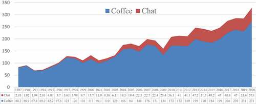
The performance of coffee and export since 1987 is depicted in Figure 1, which indicates that there has been a slight increase in the volume of export except from 2005 to 2009, where frequent ups and downs have been registered. The sharp decline in 2008 could be a response to the financial turmoil and associated decline in the performance of the world economy at the time. And a slight decline registered in 2019 could be a response to the COVID-19 pandemic. The yearly fluctuation of the export volume has been higher for coffee than for khat. In addition, no sharp increase has been registered following the devaluation measures of the government at different times. In 1987, 80.2 thousand metric tons (MT) of coffee were supplied to the international market. The figure increased to 176 thousand MT in 2007 but immediately showed a slight decline to 171 MT in 2008. And then, a rising trend was registered until 2018. On the other hand, there was a slight drop in the volume of coffee exports, which was followed by two devaluation periods (about a 27% drop in 2009 and a 0.94% drop in 2019). With the exception of a decline in trade in 2014, the performance of khat exports was relatively better following those devaluation measures.

Figure 1. Total coffee and khat export performance (in thousands of metric tone).

Source: NBE, 2020.

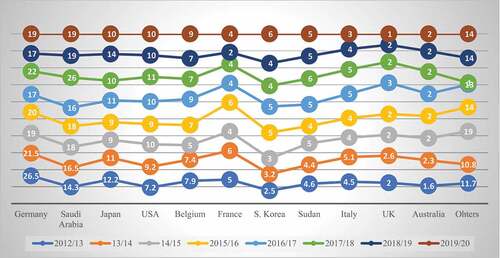
As per Figure 2, Germany has maintained the first position as an important Ethiopian coffee destination throughout the years. Saudi Arabia, Japan, and the USA are in the second, third, and fourth positions, respectively, in the last five consecutive years. Generally, the listed 11 countries consume more than 85% of Ethiopia’s total coffee exports, which in turn implies that there is market potential that the country would exploit, given that there are enough responses from the supply side. If farmers produce a high volume of coffee with high quality, it is a very profitable and advantageous business for Ethiopia’s producers, exporters, and the country as well. There is a need to educate farmers about the economic importance of coffee, as well as about the new technology. This education campaign should be complemented with the availability of high-quality planting materials and the provision of other services (especially extension) to stop the declining productivity and export earnings of our “green gold”. Educating farmers and coffee bean collectors on how to keep the quality of coffee and increase the product is an important asset. Increasing the volume as well as the quality of the coffee product throughout coffee’s potential areas may brighten the future of coffee.

Figure 2. Share of coffee export (volume) by destination (2012/13-201,920).

Source: Ethiopian Coffee and Tea Authority, 2020

On the other hand, the khat industry is one of the leading agricultural sectors. The industry constitutes 4% of the country’s export earnings and shares 9.4% of total merchandise exports (NBE, 2017). Khat (Catha edulis) is an evergreen tree cultivated for the production of fresh leaves that are chewed for their euphoric properties. The plant is well known and controversial in the eastern part of Africa and the Arabian Peninsula due to its adverse impact on one hand and its preferred crop on the other (U.S. Department of Justice, 2017). It mostly grows in East Africa and southern Arabia and is often known as chat but also goes by different names such as khat, qat, kat, Abyssinian tea, African tea, and African salad (Al-Mugahed, 2008). In Ethiopia, there are also other names given to khat, such as Aweday, Beleche, Abo Mismar, Wondo, Bahirdar, Gelemso, Hirna, etc., which are based on the source of the plant.

Currently, Ethiopia is the leading khat producer in Africa and worldwide. Most of the khat is produced in the south-eastern part of the country. Even if the khat export in some countries is banned and unpermitted to transact within and outside the country, Ethiopia constitutes one of the major earnings from khat consumption within a country and its export. The volume of khat exports increased steadily from 60 tons in 1998 to 157 tons in 2000. However, due to the shortage in supply, the revenue declined from 618.8 million ETB in 2000 to 510.5 million ETB in 2001 and 418.7 million ETB in 2002. Because of the drought and high domestic consumption, there was a shortage of plant supplies (Tolcha, 2020).

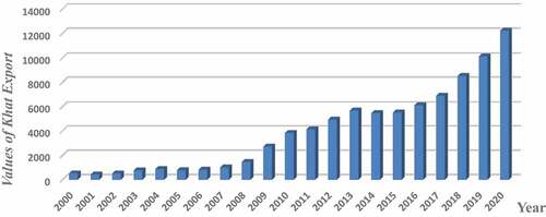
The value of khat is the most dynamic over time. The value received from exporting khat increased from 15.9 million ETB in 1985 to 618.8 million ETB in 2000 and continued to rise, reaching 6.1 billion ETB in 2017. The volume of khat exports also increased from 138 tons in 1985 to 156 tons in 2000 and reached 488 tons in 2017. This is mainly attributed to increased demand from Somalia. Somaliland is becoming the largest importer of khat, replacing Djibouti, the traditional largest importer of khat products, and it accounts for the largest share of export earnings. Khat shows remarkable growth from time to time as compared to other exported commodities. Though the plant is termed a drug of abuse, the market for the plant is worldwide. It exported too many countries to countries, including some parts of Europe, North America, Colombia, Afghanistan, Somalia, and Djibouti (Segers et al., 2005).

Khat was the most revenue-generating export in Ethiopia in 1999/2000, which generated 618.8 million ETB. It is well known that due to its high-income elasticity and its export earnings share, it rises from year to year continuously as compared to other exported commodities (see Figure 3). The revenue that the Ethiopian government got from khat export was second only to coffee export for the last six consecutive years from 1998 to 2003. According to the NBE report, its share of khat exports in total merchandise exports went up to 9.4% in 2016/17. The revenue gained from khat exports reached 1448 million ETB in 2008/09. Even if the income from khat export increases from year to year, there is no policy direction taken by the government of Ethiopia towards encouraging farmers and producers.

Figure 3. The values of khat export in million Birr.

Source: National Bank of Ethiopia and author’s computation, 2021.

2.1.2 Currency devaluation and its effect on the volume of coffee and khat export

The level of development of the economy, resource endowments, policies, and development strategies pursued are some of the determining factors of the export structure of a country. Being an underdeveloped economy that heavily depends on agriculture, the structure of Ethiopian exports is dominated by agricultural products, which used to account for more than 90% over a long period of time. In light of this fact, the Ethiopian government has devalued its currency three times in large percentages in order to increase exports and improve current account disequilibrium. As it was mentioned in the introductory part, these devaluations took place: first, on 1 October 1992, from 2.07 Birr to 5 Birr per dollar by 142%; second, on 1 September 2010, from 13.62 to 16.35 by 16.7%; and third, on 10 October 2017, from 23.4 Birr to 26.91 Birr per dollar by 15%.

Did the volume of coffee and khat exports increase after devaluation? The outcomes of the initial large devaluation: The result shows that after the application of the devaluation policy, the volume of coffee exports increased to 67,052.03 tons in 1992 as compared to that of 32,249 in 1991. Similarly, the export volume of khat increased to 1,936.40 tons in 1992 as compared to 251 tons in 1991. As shown in Table 1, the export volume of Ethiopian coffee decreased by 2809.17 after the devaluation policy was applied. This could be due to the fact that coffee farmers have been unable to make a good profit from their farms for decades. There was no concern for strong coffee institutions, lack of commitment to support the coffee sector, extreme and uncontrolled illegal market, extensive (long) coffee value chain, etc. The result for the volume of khat exports after the second devaluation shows an improvement of 81.13 tons. The result of the last devaluation reveals that in 2018, the volume of coffee exports decreased by 7641.41 tons after the devaluation policy was implemented by the government. This may be due to the fact that coffee is an agricultural commodity in which the exporters are unable to respond to international demand within a short period of time. In the case of khat, the export volume increased by 6541.2 tons, but both commodities improved in the long run.

Table 1. The volume of coffee and khat export (in metric ton) after devaluation in Ethiopia

Year	Coffee	Khat
The first devaluation and its effects on volume of commodity (in 1992 by 142 percent)
1991/92	32,249.00	251
1992/93	67,745.20	1,936.40
1993/94	69,160.00	2,808.48
1994/95	82,198.64	4,073.27
1995/96	97,578.82	3,698.29
The second devaluation and its effects on volume of commodity (in 2010)
2010/11	172,217.23	40,971.74
2011/12	169,408.06	41,052.87
2012/13	199,127.77	47,163.67
2013/14	189,669.31	51,689.76
2014/15	183,870.70	49,204.18
The last period of devaluation and its effects on volume of commodity (in 2017 by 15 percent)
2017/18	238,572.83	47,023.94
2018/19	230,931.42	53,565.13
2019/20	271,111.52	57,136.13

Source: National Bank of Ethiopia, 2020.

2.1.3. Trends of Real effective exchange rate in Ethiopia

The real effective exchange rate is defined as the units of home currency per unit of foreign currency taking account of trade partner countries trade weight and relative inflation, and the appreciation (an increase in REER) is expected to have a negative sign and reduce export. Real effective exchange rate is the most important variable of interest in this study because it is this variable which is usually used to measure the degree of international competitiveness of the country in the involvement of both bilateral and multilateral trade with the rest of the world. It follows according to this argument that a reduction in the real value of one country’s currency improves international trade competitiveness by making relatively the value of export cheaper. As a consequence, import becomes expensive and the combined effect of these things leads to the improvement of trade competitiveness and discourage import is expected to improve the trade balance.

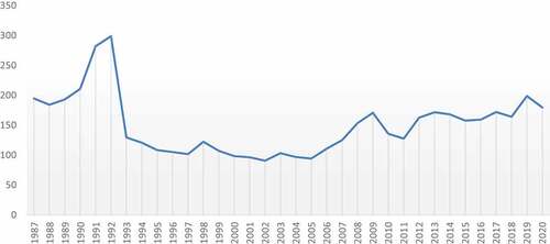
From the figure we have seen that the real effective exchange rate sharply decreased from 1992 to 1993 then slowly decreased from up the year of 2000. After 2007 tried to increase to the year of 2009 then almost remain the same between 2010 and 2011. The real effective exchange rate trends move up and down due to the price movement currency devaluation (see Figure 4). This is because the real effective exchange rate is a measure of the value of a domestic currency against a weighted average of several foreign currencies divided by a price deflator or index of costs.

Figure 4. Trends of real effective exchange rate (REER).

Source: National Bank of Ethiopia and authors’ computation, 2021.

2.2. Econometric model and estimation procedures

The response of export performance of major commodities to changes in macroeconomic variables depends primarily on whether those changes are transitory or permanent. Therefore, it is important that this decomposition is performed in the case of econometric estimation. Now, the researchers specify an econometric model that distinguishes between the permanent (trend) or transitory (short-run) components of export earnings and its macroeconomic determinants. To identify, let Y_Et be the export earnings for Ethiopia in year t and X_Et be a set of its economic determinants of major export commodity. According to Calderon et al. (2000), the permanent and transitory effects are given by

(1) $Y_{Et}=Y_{Et}^T+Y_{Et}^{P}and{X}_{Et}=X_{Et}^T+X_{Et}^P$(1)

where the superscript T represents the transitory and p represents the permanent components. A transitory fluctuation implies deviations from the trend or permanent components. Empirically, the transitory component represents short-lived fluctuations and the permanent component represents movements in the (long run) tendency of a variable. This study focuses on demand and supply side factors of Ethiopian export performance in the case of major export commodities. Here, the study shows the effect of currency devaluation on Ethiopia’s major export commodity performance. It is also affected by real GDP, the real effective exchange rate, FDI, and foreign income. In contrast to approaches followed by other empirical works on export responses to currency devaluation, in this research paper the researchers regress the exports to other explanatory variables. The empirical formulation of the model to be used in this study is given by the following function: major commodity export performance

(2) $\left(\mathrm{T}\mathrm{E}\mathrm{V}\right)=\mathrm{f}\left(\mathrm{R}\mathrm{G}\mathrm{D}\mathrm{P},\mathrm{R}\mathrm{E}\mathrm{E}\mathrm{R},\mathrm{F}\mathrm{R}\mathrm{G}\mathrm{D}\mathrm{P}\mathrm{F}\mathrm{D}\mathrm{I}\right)$(2)

Thus to determine Ethiopian major commodity export performance, a log-linear form export performance model is employed by incorporating both supply and demand-side related variables. The model is therefore similar to the one which was used by Kassa (2012) in estimating determinant of export performance in Ethiopia as well as Allaro (2012) in estimating export performance of oil seeds in Ethiopia. However, in measuring the variables, log normalization has been applied, and hence the natural logarithm forms have been taken for each variable. Therefore, the regression equation can be expressed as follows.

(3) $LnTE{V}_t=\alpha +\hspace{0.17em}{\beta }_{1}LnREE{R}_t+{\beta }_{2}LnRGD{P}_t+{\beta }_{3}LnFRGD{P}_t+{\beta }_{4}LnFD{I}_t+{\epsilon }_t$(3)

where LnTEV: Total export value of major export products in the year t in log form LnREER_t: Real Effective Exchange Rate in log form (which is found by trade weighted Birr/foreign currency)

LnRGDPt: Real gross domestic product in the log form which is a proxy for domestic national income.

LnFRGDPt: Foreign real gross domestic product in the log form which is represented by the real gross domestic product of Germany as our export destination in case of major export commodity.

LnFDI_t: The net inflow of foreign direct investment in the log form in the year t

The endogenous variable in this study is export performance of major commodities (coffee and khat). Export performance can be measured by different mechanisms. It may be measured by the total values of goods and services sold abroad in a constant price, by the total volume of goods and services sold in the external market, by its annual percentage growth or by the relative share of exported goods to a country’s total GDP. In this study, export performance of major export commodities has been measured by its total annual values in the form of natural logarithm.

2.2.1. Unit root test

It is fundamental to test for the statistical properties of variables when dealing with time series data. In level forms, time series data are rarely stationary. Regression involving non-stationary (variables that have no clear tendency to return to a constant value or linear trend) time series often leads to the problem of spurious regression. This occurs when the regression results reveal a strong and significant relationship among variables when, in fact, no relationship exists. Before conducting the simultaneous tests in the model or regression, the variables must be found to be individually stationary. Several tests are usually employed to test whether time series variables are stationary or non-stationary. The Dickey–Fuller (DF), the Augmented Dickey–Fuller (ADF) test, the Phillips–Peron test, and the Auto-Correlation Function (ACF) test. In this study, the Augmented Dickey–Fuller (ADF) test was applied to determine the existence of a unit root. The Augmented Dickey Fuller (ADF) is a test developed by Dickey and Fuller in cases where the u’s are correlated. It involves estimating the following regression:

(4) $\hspace{0.17em}{Y}_t=\hspace{0.17em}{\beta }_{1}t+\hspace{0.17em}{\beta }_{2}t+\hspace{0.17em}\delta Y_{t-1}+\sum _{i=1}^m{\alpha }_i\mathrm{\Delta }{Y}_{t-i}+{\epsilon }_t$(4)

where ε_t is a pure white noise error term, Δ is the first difference operator, while Y_t is non-stationary, its first difference is stationary where Y_t-1 = (Y_t-1—Y_t-2), Y_t-2 = (Y_t-2—Y_t-3), etc. To perform test, the number of lagged difference terms to include is often determined empirically, since it is required to include enough terms so that the error term in equation is serially uncorrelated. Determining whether a time series is stationary or not involves testing the null hypothesis δ = 0; (i.e. there is a unit root) the time series is non-stationary against the alternative hypothesis δ < 0; that is, the time series is stationary. The name unit root came from stationary series case whether the coefficient is unity or less than unity. If the null hypothesis is rejected, it means that Y_t is stationary.

The other method of unit root testing is Phillips and Perron (1988). This test is a modification and generalization of DF procedures. While DF tests assume that the residuals are statistically independent (white noise) with constant variance, Phillips–Perron (PP) tests consider less restriction on the distribution of the error or disturbance term (Enders, 2010). Phillips–Perron tests undertake non-parametric correction to account for autocorrelation present in higher AR order models. The tests assume that the expected value of the error term is equal to zero, but PP does not require that the error term be serially uncorrelated. The critical values of PP tests are similar to those given for DF tests, and this study applied both methods to have a comprehensive outcome.

If dependent and independent variables fail the stationary test, as a result, the data generating process of these variables is non-stationary. These tests are performed on both level form and the first differences between both variables. The implication of the unit root test result on the estimation procedures is that if all variables in the equation are found to be non-stationary at level form, I (0), but stationary at first difference, I (1), then a co-integration test will be conducted to find the existence of a long-run equilibrium relationship.

2.2.2. Co-integration analysis

In spite of the fact that the series is not stationary at a level, if there is a linear combination between two or more variables, the series can be stationary and there can exist a long-run equilibrium relationship among them (Gujarati, 2003). If the series are co-integrated, modeling of the long-run relationship among variables is necessary. The model to be applied in such a case is VECM, to reconcile the static long-run equilibrium relationship of co-integration with its dynamic short-run equilibrium in time series (In-Moo Kim And, G. S. M, 2006).

Two approaches are used to test the co-integration among variables: Engel and Granger (1987) and Johansen and Juselius (1990). Maximum likelihood estimation is defined by Johansen and Juselius (1990) to determine the rank of the co-integrating vector and is considered superior to the Engel and Granger (1987) approach (Shao, 2009). The normality test was undertaken on the basis of this assumption. Thus, the Johansen co-integration approach would be applied in this study. Therefore, the Johansen approach works with the formulation of a VAR system with a vector of K variables and is generated by a k-order vector autoregressive process with Gaussian errors.

(5) $Z_t=A_t{Z}_t+A_k{Z}_{t-1}+\mu +{\epsilon }_t$(5)

t = 1, 2, 3 … T, whereas Z_t is Px1 a vector of endogenous variables, A_k are the coefficient estimates and μ is the vector of Px1 constants, and Ɛ_t is error term with (0, δ).

Moreover, in the case where variables are different but stationary, it is possible to estimate the model by the first difference. However, this gives only the short-run dynamics, in which case valuable information concerning the long-run equilibrium properties of the data could be lost. In order to obtain both the short-run and long-run relationship, one can appeal to what is known as co-integration. Co-integration among the variables reflects the presence of long-term relationships in the system. In general, we need to test for co-integration because dividing the variables to attain stationarity generates a model that does not show the long-run behavior of the variables. Hence, testing for co-integration is the same as testing for long-term relationships (Gujarati, 2003). The two basic ways of testing the existence of co-integration between variables of interest and estimating the co-integrating vector are by the Engle and Granger (1987) approach and the other by the Johansen (1988) approach. However, in the case of this study, the Johansen (1998) approach was employed because it outperforms the Engle and Granger (1987) approach.

An alternative approach was proposed by Johansen (1988), who developed a maximum likelihood estimation procedure, which also allows one to test for the number of co-integrating relations. The procedure suggested by Johansen (1988) basically depends on direct investigation of co-integration in the vector autoregressive (VAR) representation. The analysis yields maximum likelihood estimators of the unconstrained co-integration vectors, but it allows one to explicitly test for the number of co-integration vectors so that the weaknesses of Engle & Granger’s (1987) two-step procedure are overcome.

Moreover, the Johansen test enables us to perform estimation and testing for the presence of multiple co-integration relationships in a single-step procedure. The Johansen method does not require a priori endogenous-exogenous distinction among variables, and it can also identify multiple co-integration vectors. The Johansen procedure sets out a maximum likelihood procedure for the estimation and determining the presence of co-integrating in a VAR system. VAR is one form of multivariate modeling where no variable in the system is assumed to be exogenous a priori. Based on this procedure, the variables of the model are represented by defining a vector of potentially endogenous variables (Anderson et al., 2009). In addition, the optimal lag length was determined based on information criteria. The objective of the information criterion (IC) method is to select the number of parameters that minimizes the value of the IC. The most popular ICs are the Akaike (1974) information criterion (AIC), Schwarz’s Bayesian information criterion (SBIC), and the Hanna-Quinn information criterion (HQIC). However, we determine the optimal lag length given the lag length selected by the majority of the criteria.

2.2.3. Vector autoregressive and vector error correction models

VAR describes the dynamic evaluation of the variables from their common history. It considers the variables in the model simultaneously and thus reduces the number of lags. It also makes more accurate forecasting possible because the included information set is extended to include the history of the other variables. The VAR model is also easy to estimate because it uses the OLS method to estimate individual equations under it and does not require division of variables. One important characteristic of the VAR process is that it generates stationary time series with time invariant means, variance, and co-variance given sufficient starting values.

The VAR approach does not require structural modeling because it treats every variable as endogenous in the system as a function of the lagged values of all endogenous variables in the system. With the objective of this study, which has to do with the interrelationship between the variables, functional relationships can be formulated in the form of vector autoregressive (VAR) equations, and VAR equations must be identified in their level form, not in their difference form. All variables have been transformed into their logarithmic form for the matter of appropriateness. Hence, log-log VAR equations can be constructed as follows:

(6) $\begin{array}{c}logE{V}_t={\beta }_o+\hspace{0.17em}\sum _{i=1}^{k-1}{\beta }_{1}logRGD{P}_{t-i}+\hspace{0.17em}\sum _{i=1}^{k-1}{\beta }_{2}logE{V}_{t-i}+\sum _{i=1}^{k-1}{\beta }_{3}logREE{R}_{t-i}\\ +\sum _{i=1}^{k-1}{\beta }_{4}logFD{I}_{t-i}\hspace{0.17em}+\hspace{0.17em}\sum _{i=1}^{k-1}{\beta }_{5}logFRGD{P_t}_{-i}+U_{2t}\end{array}$(6)

(7) $\begin{array}{c}logREE{R}_t={\alpha }_o+\hspace{0.17em}\sum _{i=1}^{k-1}{\alpha }_{1}logRGD{P}_{t-i}+\hspace{0.17em}\sum _{i=1}^{k-1}{\alpha }_{2}logE{V}_{t-i}+\sum _{i=1}^{k-1}{\alpha }_{3}logREE{R}_{t-i}\\ +\sum _{i=1}^{k-1}{\alpha }_{4}logFD{I}_{t-i}\hspace{0.17em}+\hspace{0.17em}\sum _{i=1}^{k-1}{\alpha }_{5}logFRGD{P_t}_{-i}+U_{1t}\end{array}$(7)

(8) $\begin{array}{c}logRGD{P}_t={\gamma }_o+\hspace{0.17em}\sum _{i=1}^{k-1}{\gamma }_{1}logRGD{P}_{t-i}+\hspace{0.17em}\sum _{i=1}^{k-1}{\gamma }_{2}logE{V}_{t-i}+\sum _{i=1}^{k-1}{\gamma }_{3}logREE{R}_{t-i}\\ +\sum _{i=1}^{k-1}{\gamma }_{4}logFD{I}_{t-i}\hspace{0.17em}+\hspace{0.17em}\sum _{i=1}^{k-1}{\gamma }_{5}logFRGD{P_t}_{-i}+U_{3t}\end{array}$(8)

(9) $\begin{array}{c}logFD{I}_t={\delta }_o+\hspace{0.17em}\sum _{i=1}^{k-1}{\delta }_{1}logRGD{P}_{t-i}+\hspace{0.17em}\sum _{i=1}^{k-1}{\delta }_{2}logE{V}_{t-i}+\sum _{i=1}^{k-1}{\delta }_{3}logREE{R}_{t-i}\\ +\sum _{i=1}^{k-1}{\delta }_{4}logFD{I}_{t-i}\hspace{0.17em}+\hspace{0.17em}\sum _{i=1}^{k-1}{\delta }_{5}logFRGD{P_t}_{-i}+U_{4t}\end{array}$(9)

(10) $\begin{array}{c}logFRGD{P}_t={\lambda }_o+\hspace{0.17em}\sum _{i=1}^{k-1}{\lambda }_{1}logRGD{P}_{t-i}+\hspace{0.17em}\sum _{i=1}^{k-1}{\lambda }_{2}logE{V}_{t-i}+\sum _{i=1}^{k-1}{\lambda }_{3}logREE{R}_{t-i}\\ +\sum _{i=1}^{k-1}{\lambda }_{4}logFD{I}_{t-i}\hspace{0.17em}+\hspace{0.17em}\sum _{i=1}^{k-1}{\lambda }_{5}logFRGD{P_t}_{-i}+\hspace{0.17em}{U}_{5t}\end{array}$(10)

where α_i, β_i γ_i, δ_i, and λ_i are parameters to be estimated. “i” represents individual time lag and K represents an optimal level of lag, which is determined based on information criterion, while ε_t, μ_t, ⱱ_t, η_t, Ư_t, and Ƃ_t represent white noise, innovations.

The VAR model is a general framework used to show the dynamic interrelationship among stationary variables. However, since the time series is not stationary, the VAR specified above needs to be modified to allow consistent estimators of the relationship among the variables. After testing the long-run relationship among the variables by the Johansen co-integration test, the next task is developing a vector error correction model (VECM). In order to capture both short-run and long-run relations in the models, the study utilizes the Vector Error Correction Model (VECM), a special case of the VAR for variables in their first differences. VECM also takes co-integration among the variables under consideration. If there is a long-run relationship among the variables, an ECM can be formulated to show the long-run interaction between variables (Verbeek, 2008). Once the long-run co-integration test is confirmed, the vector error correction model (VECM) that indicates the short-run dynamics parameters (the speed of adjustments by which any shocks in the short run are converged to long-run equilibrium) is followed.

In order to derive vector error correction model from the VAR model, we change the above VAR equations into their respective first difference and the lag of error correction term. The VECM for the purpose of the study can be set up as:

(11) $\mathrm{\Delta }log{Y}_t=\theta +\sum _{i=1}^{k-1}{\beta }_i\mathrm{\Delta }log{X}_{t-1}+\mathrm{\Omega }ET{C}_{t-1}+u_t$(11)

where k-1 = shows that the lag length is reducedby 11 from the VAR model ß_i = short-run dynamic coefficients of the model adjustment to long-run equilibrium. Ω = speed of adjustment parameter. ETC_t-1 = the error correction term is the lagged value of the residual obtained from the co-integrating regression of the dependent variables on the repressors. u_t = residual and often called white noise, stochastic error terms, impulses, innovations, or shock. The above equation is obtained by subtracting y_t-i from both sides of reduced form of VAR equation. This VECM is composed by first differenced variables on the LHS and k-1 lags of the dependent variables (differences) on the RHS, each with a ß short-run coefficient matrix. Ω consists on a long-run coefficient matrix, because in equilibrium, all ∆y_t-i = 0, and establishing u_t with the expected value of zero it implies that ΩETC_t-k = 0.

(12) $\begin{array}{c}\mathrm{\Delta }logE{V}_t={\beta }_o+\sum _{i=1}^{k-1}{\beta }_1\mathrm{\Delta }logRGD{P}_{t-i}+\sum _{i=1}^{k-1}{\beta }_2\mathrm{\Delta }logE{V}_{t-i}+\sum _{i=1}^{k-1}{\beta }_3\mathrm{\Delta }logREE{R}_{t-i}\\ +\sum _{i=1}^{k-1}{\beta }_4\mathrm{\Delta }logFD{I}_{t-i}+\sum _{i=1}^{k-1}{\beta }_5\mathrm{\Delta }logFRGD{P_t}_{-i}+{\mathrm{\Omega }}_{2}ET{C}_{t-1}+U_{2t}\end{array}$(12)

(13) $\begin{array}{c}\mathrm{\Delta }logREE{R}_t={\alpha }_o+\sum _{i=1}^{k-1}{\alpha }_1\mathrm{\Delta }logRGD{P}_{t-i}+\sum _{i=1}^{k-1}{\alpha }_2\mathrm{\Delta }logE{V}_{t-i}+\sum _{i=1}^{k-1}{\alpha }_3\mathrm{\Delta }logREE{R}_{t-i}\\ +\sum _{i=1}^{k-1}{\alpha }_4\mathrm{\Delta }logFD{I}_{t-i}+\sum _{i=1}^{k-1}{\alpha }_5\mathrm{\Delta }logFRGD{P_t}_{-i}+{\mathrm{\Omega }}_{1}ET{C}_{t-1}+U_{1t}\end{array}$(13)

(14) $\begin{array}{c}\mathrm{\Delta }logRGD{P}_t={\gamma }_o+\sum _{i=1}^{k-1}{\gamma }_1\mathrm{\Delta }logRGD{P}_{t-i}+\sum _{i=1}^{k-1}{\gamma }_2\mathrm{\Delta }logE{V}_{t-i}+\sum _{i=1}^{k-1}{\gamma }_3\mathrm{\Delta }logREE{R}_{t-i}\\ +\sum _{i=1}^{k-1}{\gamma }_4\mathrm{\Delta }logFD{I}_{t-i}+\sum _{i=1}^{k-1}{\gamma }_5\mathrm{\Delta }logFRGD{P_t}_{-i}+{\mathrm{\Omega }}_{3}ET{C}_{t-1}+U_{3t}\end{array}$(14)

(15) $\begin{array}{c}\mathrm{\Delta }logFD{I}_t={\delta }_o+\sum _{i=1}^{k-1}{\delta }_1\mathrm{\Delta }logRGD{P}_{t-i}+\sum _{i=1}^{k-1}{\delta }_2\mathrm{\Delta }logE{V}_{t-i}+\sum _{i=1}^{k-1}{\delta }_3\mathrm{\Delta }logREE{R}_{t-i}\\ +\sum _{i=1}^{k-1}{\delta }_4\mathrm{\Delta }logFD{I}_{t-i}+\sum _{i=1}^{k-1}{\delta }_5\mathrm{\Delta }logFRGD{P_t}_{-i}+{\mathrm{\Omega }}_{4}ET{C}_{t-1}+U_{4t}\end{array}$(15)

(16) $\begin{array}{c}\mathrm{\Delta }logFRGD{P}_t={\lambda }_o+\sum _{i=1}^{k-1}{\lambda }_1\mathrm{\Delta }logRGD{P}_{t-i}+\sum _{i=1}^{k-1}{\lambda }_2\mathrm{\Delta }logE{V}_{t-i}+\sum _{i=1}^{k-1}{\lambda }_3\mathrm{\Delta }logREE{R}_{t-i}\\ +\sum _{i=1}^{k-1}{\lambda }_4\mathrm{\Delta }logFD{I}_{t-i}+\sum _{i=1}^{k-1}{\lambda }_5\mathrm{\Delta }logFRGD{P_t}_{-i}+{\mathrm{\Omega }}_{5}ET{C}_{t-1}+U_{5t}\end{array}$(16)

where ETCt-1 is the lagged error correction term departure from the long-run co-integrating relations between these five variables. The above equations constitute a vector auto-regression model (VAR) in its first difference, which is a VAR type of ECM. Therefore, a VECM is a VAR in its first difference form with the addition of a vector of co-integrating residuals.

2.3.4. Granger causality test

Granger causality test is going to be performed in the study to identify the direction of causality. The term Granger causality has been used in the context of testing the existence of causality from exchange rate to total value of major export commodities, Real gross domestic product, Foreign direct investment, Foreign income, and vice versa, and from all these variables to exchange rate itself.

Hypothesis: Ho = Real exchange rate does not Granger cause export performance of Ethiopia

H₁ = Real exchange rate Granger causes the export performance of Ethiopia.

Decision rule: if the probability of the significance level is less than 5%, we can reject the null hypothesis which claims no Granger causality and if not, we accept the null hypothesis. If there is Granger causality from real exchange rate to export performance of major commodities and from export performance of major commodities to real exchange rate, we call it bidirectional causality.

3. Findings and discussions

3.1. Stationarity of data

Stationarity is an important concept that plays an important role when estimating time series analysis. Proper estimation of a time series model requires stationary data. Conducting time series analysis on non-stationary data will result in what is called “spurious“ or ”nonsense” regression. This occurs when the regression results reveal a strong and significant relationship among variables, when in fact, there is no relationship that exists. Before conducting the simultaneous tests within the model or regression, the variables must be found to be individually stationary. Therefore, the initial task we must undertake before any regression in secondary time series data is testing for stationarity of data. In the following table, the Augmented Dickey–Fuller (ADF) test is used to check whether the data at hand get stationary or not.

As we can see, from Table 2 of the ADF results of lnTEV, lnREER, lnRGDP, lnFRGDP, and lnFDI, the absolute value of each of the t statistics is smaller than the absolute values of each of the critical values at a level. For instance, in the case of lnTEV, the t-statistic is equal to −1.226233, which is less than −2.954021. In addition to the t-stat, the p-value of the variable is not significant since its value is greater than 5%. Therefore, it is possible to accept the null hypothesis, which claims that variables have a unit root at level. The same is true in the case of lnREER, lnRGDP, lnFRGDP, and lnFDI, as shown on the left-hand side of the table 2.

Table 2. Augmented Dickey–Fuller unit root test

	Augmented Dickey-Fuller test
	At level			At first difference			Order of integration
Variables	T-test	Crit. value	P-value	T-test	Crit. value	P-value
lnTEV	−1.22623	−2.95402	0.6511	−7.29019	−2.95711	0.0000	I(1)
lnREER	−1.85786	−2.95402	0.3472	−5.21319	−2.95711	0.0002	I(1)
lnRGDP	1.880279	−2.95402	0.9997	−4.67119	−2.95711	0.0007	I(1)
lnFRGDP	−2.43018	−2.95402	0.1416	−5.23389	−2.95711	0.0002	I(1)
lnFDI	−2.39337	−2.95402	0.1512	−4.80380	−2.95711	0.0005	I(1)

Source: The results are calculated by the author using Eviews 10.0 software, 2021.

Since the variables have unit root, it is impossible to estimate the model directly and we need to fix the problem by taking the first difference of the variables and checking again if they are stationary. The original data needs to be changed to its first difference and the ADF test needs to be checked once again. Hence, we continue the analysis by taking the first difference, so that we can determine in which order the variables become stationary. When we look at the results of ADF tests conducted on the difference of the variables on the right-hand side of the table, the null hypothesis of unit root is strongly rejected. Thus, we can conclude that all variables are stationary at the first difference. Since all variables are I (1), it is possible to use the Johansen co-integration approach. Once the stationarity test is checked and confirmed, the next step is choosing the optimal lag selection, which determines the number of the co-integrating equation.

3.2. Determination of optimal lag length

Before going to check for the multivariate time series analysis, choosing the optimal lag length for the basic VAR model in advance is needed. It is obvious that the result of the Johansen co-integration test is very sensitive to optimal lag length. To determine the optimal lag length, different information criteria have been employed. The objective of the information criteria (IC) method is to select the number of parameters that minimizes the value of the IC. The most popular information ICs are the Akaike information criterion (AIC), Schwarz’s Bayesian information criterion (SIC), and the Hannan-Quinn information criterion (HQIC). Practically, the optimal lag length, which is selected by most of these criteria, is going to be included in the VAR system.

In order to test co-integration, it is necessary to specify the number of lags to be included in the model. As stated above, the optimal lag length must be determined by the lag selected by the most information criterion. According to Table 3, almost all criteria choose three lags, and only LR and SC choose two lags and one lag, respectively. Therefore, the optimal lag for the underlying VAR model is three.

Table 3. VAR optimal lag selection

Lag	LogL	LR	FPE	AIC	SC	HQ
0	−35.10675	NA	0.000159	2.607117	2.793943	2.666884
1	85.56044	201.1120	1.50e-07	−4.370696	−3.436565*	−4.071859
2	106.5806	29.42817*	1.15e-07	−4.705371	−3.023934	−4.167465
3	128.0060	24.28212	9.46e-08*	−5.067064*	−2.638322	−4.290088*
4	143.6500	13.55821	1.39e-07	−5.043336	−1.867289	−4.027292

* indicates lag order selected by the criterion.

LR: sequential modified LR test statistic (each test at 5 percent level); FPE: Final prediction error; AIC: Akaike information criterion; SC: Schwarz information criterion; HQ: Hannan-Quinn information criterion.

3.3. Co-integration test

After completion of the unit root test and determination of optimal lags to be included in the model, the third step is testing for co-integration. If the variables are found to be co-integrated, it means that there exists a linear, stable, and long-run relationship among them, such that the disequilibrium errors would tend to fluctuate around zero mean. In the literature, co-integration tests, for instance, Engle and Granger (1987), Johansen (1988), Johansen and Juselius (1990), and Pesaran et al. (2001), are used to confirm the presence of a potential long-run equilibrium relationship between two variables. The current study used Johansen’s technique in order to establish how many co-integrating equations exist between variables.

The Johansen test can be seen as a multivariate generalization of the augmented Dickey–Fuller test. The generalization is the examination of linear combinations of variables for unit roots. The Johansen test and estimation strategy is maximum likelihood. This makes it possible to estimate all co-integrating vectors when there are more than two variables. If there are three variables each with unit roots, there are at most two co-integrating vectors. More generally, if there are n variables which all have unit roots, there are at most n1 co-integrating vectors. Accordingly, the trace and maximum eigenvalue test statistics have rejected the null of no-co-integration among the series of interest while confirming the existence of long-run relationships among them. The summary statistics of both tests are reflected in Table 4;

Table 4. Johansen co-integration test (trace and eigen value test)

Max rank	Eigen values	Trace test			Eigen value
		Trace statistic	Critical values (0.05)	Prob.	Max-eigen statistic	Critical values (0.05)	Prob.
0	0.93	188.95	69.81	0.00	84.31	33.87	0.00
1	0.83	104.63	47.85	0.00	54.56	27.58	0.00
2	0.61	50.07	29.79	0.00	28.43	21.13	0.00
3	0.48	21.64	15.49	0.00	19.77	14.26	0.00
4	0.06	1.86	3.84	0.17	1.86	3.84	0.17

Source: The results are calculated by the author using Eviews 10 software, 2021.

Table 4 revealed the existence of co-integration by a trace statistics test at a 5% level. According to Johansen co-integration, maximum rank represents the number of co-integrating equations in the system. At maximum rank zero, the null hypothesis says there is no co-integration among the variables, whereas the alternative hypothesis says there is at least a co-integration among them. To determine the presence of co-integration, the trace statistics must be compared with the critical value at a 5% significance level. In the above-computed table, the trace statistics are greater than the critical value at 5% level of significance, and thus we can confidently reject the null hypothesis of no co-integration. However, at maximum rank 4, the trace statistics are less than the critical value at the 5% level of significance, so we accept the null hypothesis.

Maximum Eigenvalue revealed that at the maximum rank of zero, one, two, and three, their maximum Eigen values are greater than the critical value at the 5% level of significance. Therefore, these two tests confirm a co-integrating relationship among total export value, real effective exchange rate, real gross domestic product, foreign real gross domestic product, and foreign direct investment. The model should be considered the target model, and the dependent variable of that model should be the target variable of this study. Therefore, from the evidence of the long-run associations, we can run a vector error correction model (VECM).

3.4. Vector error correction model (VECM) results and analysis

After the evidence of co-integration relationship among the variables has been checked, the next step is obviously to run the vector error correction model (VECM) using one less lag length (p-1). p is the optimal lag length determined with vector autoregressive (VAR). Hence, the optimal lag length of the model was 3, and therefore the vector error correction model (VECM) requires 2 lag length to run a regression.

3.4.1. The long-run model

Given the finding from the Johansen’s co-integration test, we understand that LTEV, LRGDP, LREER, LFRGDP, and FDI are co-integrated in the long run. We utilize the co-integrating vector to construct the vector error correction model (VECM). Table 5 shows the Vector Error Correction Estimates of total export value as an endogenous variable. In the long run, elasticities have been exactly identified and the Johnson normalization restrictions have been imposed too. The long-run result relationship is depicted in the table 5.

Table 5. Long-run relationship of co-integrated vector

Regressors	Coefficient	Standard deviation	t-statistics
lnREER	4.620439	1.43315	−3.22397*
lnRGDP	−0.558702	0.27724	2.01525*
lnFRGDP	0.007214	0.05042	−0.14308
LnFDI	0.288340	0.07894	−3.65247*
C	−2.747368

Source: Author’s computation using EVIEWS 10 software, 2021.

*indicates the significance of the coefficients (the rejection of the null hypothesis) at 5%.

Table 5 shows the Vector Error Correction Estimates of total export value as an endogenous variable. The long-run elasticities were exactly identified, and the Johnson normalization restrictions were imposed. The result in Table 5 shows that, except for lnFRGDP, all variables are statistically affecting the total export value of major export commodities in Ethiopia. Each variable, except foreign income, in the long run, significantly affects the export performance of major export commodities. In general, the long-run equation of the model between the regressors and total export value would be written with the respective t-ratio in parenthesis as follows.

(18) $\begin{array}{c}\mathrm{L}\mathrm{n}\mathrm{T}\mathrm{E}\mathrm{V}=-2.747368+4.620439\mathrm{l}\mathrm{n}\mathrm{R}\mathrm{E}\mathrm{E}\mathrm{R}-0.558702\mathrm{l}\mathrm{n}\mathrm{R}\mathrm{G}\mathrm{D}\mathrm{P}+0.007214\mathrm{l}\mathrm{n}\mathrm{F}\mathrm{R}\mathrm{G}\mathrm{D}\mathrm{P}+0.288340\mathrm{l}\mathrm{n}\mathrm{F}\mathrm{D}\mathrm{I}\\ \left[-3.22397\right]\left[2.01525\right]\hspace{0.17em}\left[-0.14308\right]\left[-3.65247\right]\end{array}$(18)

The result of this equation shows that real effective exchange rate is positive as expected in the literature part and significantly affects the total export value of Ethiopia. This implies that policy measures regarding the exchange rate have paramount importance in improving major commodity exports. The result is in line with the findings of Kayamo (2019), in that he claims real effective exchange rate has positive effect on the export earnings in Ethiopia. Also, the result is similar to that of Dube et al. (2018) where the exchange rate positively and significantly affects the export performance of agricultural export in Ethiopia. Therefore, keeping the effect of other things as constant, increasing the exchange rate or devaluation of domestic currency by 1% improves total export value of Ethiopia’s major export commodity by 4.62% in the long run.

The impact of foreign real GDP on the export performance of major export commodities is statistically insignificant. The result is in line with Anagaw and Demissie (2012) for Ethiopia, where the increase or decrease in a trading partner’s real gross domestic product for Ethiopian export performance was statistically insignificant. Moreover, the finding is similar to the results of Amin (2007) and Narayan & Narayan (2010), where the demand for our exports by the trading partners doesn’t respond to the change in their income level. Consequently, the finding confirms the proposition that most agricultural products’ export demand is income inelastic in their very nature. Also, the result goes with that of Kayamo (2019) in that the real income of trading partners has a dominant effect on the Ethiopian export earnings of coffee.

There is significant relationship between foreign direct investment and export value in Ethiopia. The result reveals that where FDI does contribute to the technological upgrading and structural evolution of the export sector, the structure of the sector is an important ingredient at any stage. Thus, export performance positively responds to FDI in the long run. The finding is in line with that of Fenta and Menber (2018) in his claims of the positive relationship between the export earnings in the long run. Therefore, keeping the effect of other things remains the same, the 1% increase in foreign direct investment will result in a 0.29% increase of total export value of major export commodity in the long run.

In case of real domestic income, the sign of real gross domestic product is opposite sign from the anticipated, but it is statistically significant. This negative relationship might be justified in such a way that when GDP of the country increases, domestic absorption will definitely increase. If domestic absorption increases, it is obvious that export of major export products will decrease. Other things being constant, 1% increase in real gross domestic product leads to 0.5587% decrease in the export performance of Ethiopia’s major export commodity. This finding is also similar to that of Fenta and Menber (2018) in that real gross domestic product with unexpected negative sign, which is negatively related and statistically significant in explaining export in the long run. Another justification with regard to domestic real income the result revealed that the domestic real income has negative effect on the export performance of Ethiopia in case of major commodity. This means that when the domestic real income increases, domestic consumers will increase their consumption of imported goods.

3.4.2. The short-run dynamics for vector error correction model

After the estimation of long-run coefficients, the next step is to estimate the short-run ECM model. The coefficient of error correction term (ECM) as discussed in the methodology part indicates the speed by which any deviation in the short-run from equilibrium is restored to equilibrium in the dynamic model. The coefficient of the ECM is obtained from the regression of one lagged period residual of the dynamic long-run model. The coefficient of the error correction (ECM) term, thus, indicates how quickly variables converge to their equilibrium. The short-run relationship between the exchange rate devaluation, total export value, foreign real gross domestic product, real gross domestic product, and foreign direct investment can be shown by the vector error correction model. Moreover, to have this function, it should have a negative sign and be statistically significant at a standard significant level, which means its p-value (probability value) must be less than 5% level of significance.

According to Banerjee et al. (1993), the highly significant error correction term further confirms the existence of a stable long-run relationship. As reported in Table 6, the error correction coefficient of the estimated result is −0.3088, which is statistically significant because it has the desired negative sign and implies a high speed of adjustment in which the system is restored to its long-run equilibrium. The coefficient of the speed of adjustment is negative and, as desired, statistically significant, which shows that the deviation by any of the explanatory variables in the short run would be corrected by the speed of 30.88% in the long run per year. This means that the shocks/deviation of each explanatory variable on total export value would move towards long-run equilibrium by 30.88%.

Table 6. Short-run dynamics of VECM

Model, VECM	Coefficients	Standard error	t-Statistic	P-value
cointEq1	−0.308818*	0.101640	−3.038364	0.0068*
D(LTEV(−1))	−0.164813	0.198783	−0.829109	0.4173
D(LTEV(−2))	0.202650	0.213683	0.948368	0.3548
D(LREER(−1))	−0.604585	0.480026	−1.259482	0.2231
D(LREER(−2))	−0.176349	0.332505	−0.530367	0.6020
D(LRGDP(−1))	0.188690	0.464295	0.406402	0.6890
D(LRGDP(−2))	0.487889	0.491414	0.992827	0.3333
D(LFRGDP(−1))	0.052183*	0.019279	2.706727	0.0140*
D(LFRGDP(−2))	0.0074226	0.026398	0.281290	0.7815
D(LFDI(−1))	0.091497*	0.040163	−2.278151	0.0345*
D(LFDI(−2))	−0.014983	0.046140	−0.324720	0.7489
C	0.006749	0.046555	0.144972	0.8863
R-squared	0.632171	Mean dependent var		0.021339
Adjusted R-squared	0.419217	S.D. dependent var		0.138280
S.E. of regression	0.105382	Akaike info criterion		−1.377811
Sum squared resid	0.211000	Schwarz criterion		−0.822720
Log likelihood	33.35608	Hannan-Quinn criter.		−1.196865
F-statistic	2.968581	Durbin-Watson stat		1.873040
Prob(F-statistic)	0.018123

Source: Author’s computation, 2021. *indicates the significance of the coefficients (the rejection of the null hypothesis) at 5%.

In other words, the error correction term, which measures the speed of adjustment to long-run equilibrium, is important to the analysis in the VECM’s results. The error correction term is significant, has the correct negative sign (stable adjustment coefficients that move back to equilibrium), and the value of the term lies within the relevant range of 0 and −1 as required. The results based on the above result of the error correction term show that about 30.88% of the disequilibrium in the total export value is corrected each year. This means that any deviation in the short run from the equilibrium level of total export value in the current period is converged to equilibrium by 30.88% per annum to bring back equilibrium when there is a shock to a steady state relationship. The significance of coefficients at a 5% level is indicated by all coefficients whose probability is denoted by the * symbol.

According to the estimation result, there is a positive and significant association between the export performance of major commodities and foreign real income as it is hypothesized that when the demand for Ethiopian major commodities increases with the income of trading countries, the export earnings and performance also increase. The findings are consistent with the findings of Kayamo (2019), who argued that the real income of trading countries has a significant relationship with export earnings in Ethiopia, as well as Muthamia and Muturi (2015), who discovered that the real income of trading partners has a positive and significant effect on export volume in Kenya.

Foreign direct investment also positively and significantly affects the export earnings of major export commodities in Ethiopia by its first period lags as theoretical expectation. It was revealed to be significant in both the short run and long run. Foreign direct investment (FDI) is statistically significant at a 5% level. A positive and significant relationship between export performance of major commodities and FDI in Ethiopia indicates that the contribution of FDI to capital formation helps to increase the performance of exports in Ethiopia. Thus, export performance positively responds to FDI in the short run. The finding is similar to the finding of Dube et al. (2018) in that both in the short run and the long run, export performance is affected by foreign direct investment in Ethiopia.

Moreover, there is a positive relationship between real income and total export value of major export commodity as expected sign that implies the higher income the citizens have the ability to produce and export which it leads to higher export earnings, however it is statistically insignificant. The study came up with the result that there is a negative short-run and a positive long-run relationship between the total export value of export in Ethiopia and real exchange rate. This may reflect the existence of the J-curve effect, as the Ethiopian major commodity export value first deteriorates after currency depreciation and then it improves in the long run.

However, if the J-curve effect is maintained, the real effective exchange rate is statistically not affected by the export performance of major commodities in the short run. This result is similar to the findings of Kayamo (2019) and Narayan (2013), in that the exchange rate exhibits a J-curve effect on the export earnings of Ethiopia. Moreover, the result is in line with that of Fanta and Teshale (2013) in that their Johansen co-integration test and Vector Error Correction model proved that the real exchange rate has a statistically significant negative long-run effect on exports but not in the short run.

Generally, most of the exports of Ethiopia are primary commodities produced by the agricultural sector. It is true that the production or supply of agriculture sector is not elastic in responding to changes in exchange rate as it takes some time to produce the commodities and the Ethiopian export sector cannot respond foreign demand immediately within short period of time. Means that Production does not respond immediately to changes in real effective exchange rate or currency devaluation, and the policy of government is not effective in the short run. Similarly, import demands for developing countries like Ethiopia, are inelastic as their imports are primarily composed of capital goods, semi-finished goods, fuels, and the like of which, a nation cannot cut their imports.

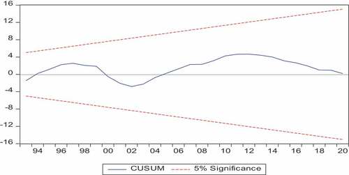
3.4.3. Stability of the VEC model

Stability diagnostics to measure parameter reliability or uniformity are a critical issue for total export value equations. In particular, to be able to interpret the estimated equation as an export performance equation, it is necessary to ensure that the parameters are stable over the estimation period. To achieve this, the study implemented the cumulative sum (CUSUM) tests. The decision about the parameter stability relies on the position of the plot relative to the 5% critical bound. The CUSUM test is based on the cumulative sum of recursive residuals given below in the following figure. For stability of the short-run dynamics and the long-run parameters of the model, it is important that the blue trend line has to be drawn between the two red lines as shown in Figure 5. Therefore, the model is said to be dynamically stable because the blue trend line lies between the red lines and also because the blue trend line is far away from the borderline.

Figure 5. The stability of VEC model.

Source: Own computation, 2021.

3.5. Granger causality test

Granger causality test is a statistical hypothesis test for determining the usefulness of one time series in forecasting another time series. The causality test is used to measure the ability to predict the future values of a time series on the basis of the previous values of another time series. Granger causality in a VAR model implies a correlation between current values of one variable and the past values of other variables. Recall that although there is co-integration between two variables does not specify the direction of a causal relationship between variables, economic theory guarantees that there is always Granger causality in at least one direction. Researchers verify the direction of Granger causality between variables. The study used chi-square statistics and probability to measure causality between variables.

Hypothesis testing:H0 – There is no Granger causality from REER to TEV

H1 – There is Granger causality from REER to TEV

A significant probability value of 5% indicates that the null hypothesis is rejected statistically. There are two types of causality running: unidirectional causality and multi-directional causality. If real effective exchange rate (REER) Granger causes total export value (TEV) but total export value does not cause real effective exchange rate, we say that there is only unidirectional causality from real effective exchange rate to total export value at the appropriate significance level. In that case, the multi-causality would run if there was a causality from real effective exchange rate (REER) to total export value (TEV) and vice versa. In this study, the estimation results for Granger causality between each variable are presented in Table 7.

Table 7. Pairwise Granger causality test

Null hypothesis	Observation	F-statistic	P-value
LREER does not Granger Cause LTEV	32	8.78624	0.0012*
LTEV does not Granger Cause LREER		0.38439	0.6845
LRGDP does not Granger Cause LTEV	32	1.78930	0.1863
LTEV does not Granger Cause LRGDP		4.28973	0.0241*
LFRGDP does not Granger Cause LTEV	32	5.26309	0.0117*
LTEV does not Granger Cause LFRGDP		0.10127	0.9040
LFDI does not Granger Cause LREER	32	16.7888	2.E-05*
LREER does not Granger Cause LFDI		0.88193	0.4256
LFDI does not Granger Cause LRGDP	32	3.83526	0.0342*
LRGDP does not Granger Cause LFDI		0.96470	0.3938

Source: Own computation using EVIEWS 10 software, 2021. *indicates the significance of the coefficients (the rejection of the null hypothesis) at 5%

From Table 7, we can understand that LREER Granger causes LTEV as shown and that the probability value of F-statistics is significant because it is less than 5%. Therefore, we can reject the null hypothesis (H0) that states’ real effective exchange rate does not Granger cause total export value variable and we accept the alternative hypothesis that real effective exchange rate Granger causes the total export value. Also, we can judge that LFDI Granger causes LRGDP in that its probability value of F-statistics is less than 5%. Generally, we can conclude that in this model there is only unidirectional causality between variables and no multi-directional causality.

3.6. Variance decomposition (VD)

The variance decomposition provides information about the relative importance of each orthogonal zed random innovation in affecting the variation of the variables in each forecast error. The forecast error variance decomposition for each variable reveals the proportion of the movement in these variables due to their own shocks versus the shocks in other variables. In other words, variance decomposition gives the proportion of the movements in the dependent variables that are due to their “own” shocks (innovations) versus shocks to the other variables (Tursoy, 2019). Based on the result, the variance decomposition of total export value as a variable endorsed to its own innovation and to shocks in the other variables for a forecast horizon of 1 through 10 years is presented below under Table 8.

Table 8. Variance decomposition of total export value

Period	S.e	LTEV	LREER	LRGDP	LFRGDP	LFDI
1	0.105382	100.0000	0.000000	0.000000	0.000000	0.000000
2	0.138768	82.61380	5.525700	0.940336	10.90801	0.012155
3	0.193070	77.29081	6.153133	1.240613	10.14045	5.174996
4	0.230832	71.07031	5.586979	1.754849	12.41516	9.172696
5	0.280758	68.36372	4.019843	1.200397	15.91898	10.49705
6	0.319491	66.33599	3.632886	1.005472	17.40309	11.62256
7	0.358304	67.31343	3.028538	0.941199	17.40962	11.30721
8	0.390854	67.12782	2.716545	0.942781	18.13774	11.07511
9	0.422307	67.32937	2.566819	0.888909	18.01373	11.20117
10	0.449410	66.96576	2.492646	1.003907	18.15241	11.38527

Source: Own computation using EVIEWs software, 2021.

This result showed that, in the short run, 100% of the forecast error variance in total export value is explained by itself. We can say that it is strongly endogenous. In other words, the variation in the total export value is caused by its own innovation and which accounts for 100% of it. This decreases to about 82.61% in the second year and continues to decline gradually over time as this is offset by the importance of other independent variables in the system. The real effective exchange rate explains only 5.527% of the forecast error variation in the total export value, and the source of variation is foreign income, which covers about 10.90% of the total export value, whereas domestic income and foreign direct investment have a limited percentage of the total export value.

In the third period, the shock of the exchange rate on total export value forecast variation is 6.153%, whereas the foreign income shock to the total export value is about 10.14%. In this period, both domestic income and foreign direct investment comprised 1.24% and 5.17%, respectively. In the 10th year, in Ethiopia, the significant source of variation in the total export value forecast error is its own innovations, and its average rate of progress is 66.96% in the forecast horizon. The real exchange rate innovation explains about an average of 2.49% of the variation in the total export value of Ethiopia’s major export commodities, whereas innovation in foreign real income causes the variation in total export value by 18.15%.

The result of the model suggested that the effect of foreign direct investment and foreign income on the export performance of Ethiopia’s major export commodities appears to be significant. The series of foreign direct investment and foreign income have been increasing throughout the years, thus exerting a strong endogenous influence on total export value.

3.7. Impulse response function

Impulse response functions are performed to provide more insights into the dynamics of the explanatory variables. It is used to point out the effect of a one-standard deviation shock to one of the innovations on current and future values of the endogenous variables. In this study, special attention is given to the real exchange rate, which is a key independent variable that affects the export performance of total export values of commodities. The following Cholesky order is employed. Figure 6 shows how the total export value of major commodities responds to a one-standard deviation of the independent variables at any point in time.

Figure 6. Impulse response of total export value.

Source: Author’s computation using STATA software, 2021.

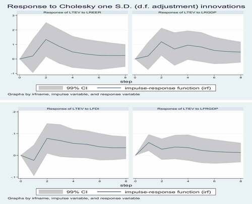
As the figure depicts, after the shock of REER, the total export value of major commodities improves up to the second year and remains the same between the third and fourth years. After the seventh year, it starts to improve when the number of years increases. On average, a one percent real depreciation of the Ethiopian Birr relative to a trading country’s currency has a long-run positive impact on the export performance of major commodities. However, the total export value of major commodities responds negatively to a shock in real gross domestic product up to the second year, and it starts to improve only after a very few years in that the increase in this year does not offset the deterioration of the coming years. This implies that the effect of real income on the export performance of major commodities is negative, which confirms the long-run results of the VEC model. As the figure clearly shows, the response of export performance to a shock of both foreign income and foreign direct investment is positive. It revealed that the effects of foreign income and foreign direct investment on the export performance of major commodities in Ethiopia are positive and significant in the long run.

Overall, the estimated long-run coefficients obtained from the co-integrating equations confirm the results that correspond to the long-run findings of the impulse response functions, such that positive relationships exist between the total export value of major export commodities and the REER, as well as the total export value and foreign direct investment. The findings are also similar in estimating the negative relationship found between the total export value and domestic income.

4. Conclusion and recommendation

Devaluation of the currency has been stipulated and is being utilized increasingly as the main stabilization device in developing countries as part of International Monetary Fund (IMF) mainstream adjustment programs. The policy measure of currency devaluation has aimed to make export products more competitive and permute demand towards domestically produced goods, eventually boosting the overall output of the country. Further, devaluation or depreciation of the exchange rate is expected to improve the international competitiveness of the devaluing or depreciating country by changing the relative price of home and foreign goods. Based on this obvious reasoning, the government of Ethiopia engaged in a continuous currency devaluation policy to improve its export performance. Unfortunately, no promising results have been recorded so far in terms of boosting export performance as well as improvement in its external balance. That is the core reason that motivated the researchers to examine the effect of currency devaluation on major export commodities (coffee and khat) in Ethiopia.

Moreover, the main research question this study seeks to answer is whether currency devaluation significantly affects the export performance of major export commodities in Ethiopia. In order to achieve this objective, time series data ranging from the year 1987 up to 2020 from different sources have been employed. In this study, the values of major export commodities were used as dependent variables, while explanatory variables included the real effective exchange rate, foreign real gross domestic product, real gross domestic product, and foreign direct investment.

Employing Johansen co-integration, VECM, and impulse responses, the study found that the short-run effects of the REER on the export value of major commodities are different from the long-run effects. In particular, it is found that the REER is negatively and insignificantly related to the total export value of major export commodities in the short run, while a positive and significant relationship exists in the long run. It implies that a decrease in the external value of the domestic currency initially causes a deterioration; however, a short-run currency devaluation has no effect on Ethiopia’s export performance of major commodities and leads to an improvement thereafter.

The movement in the real effective exchange rate has also appeared to have a positive relationship with export performance. Real effective exchange rate movements are positively related to the growth in export performance in the long run. An increase in the real effective exchange rate means a real depreciation of the domestic currency, which makes exportable items cheap. According to this study, a 1% change in the real effective exchange rate results in a 4.12% change in total export earnings. It is well known that the exports of developing countries are price inelastic in the international market due to the nature of the products that LDCs produce. Hence, this result is consistent with this fact. It follows that devaluation of birr in terms of foreign currency improves the price competitiveness of exports and hence leads to an increased export performance of Ethiopia in the long run.

The study further came up with the finding that there is a long-run negative and significant relationship between real domestic income and export performance, indicating that a rise in real domestic income leads to a decrease in the export performance of major commodities in Ethiopia. The negative sign of the coefficient of real domestic income supports the Keynesian view or absorption approach that increases in domestic real income will encourage citizens to buy more imported goods and thus decrease export performance in the long run. This means that higher domestic income will lead to higher demand for foreign goods and, thereby, lower saving in the country, which results in low investment and low exports. The main reason is that import demands for developing countries like Ethiopia are inelastic as their imports are primarily composed of capital goods, semi-finished goods, fuels, and the like, without which a nation cannot cut their imports.

In contrast, a long-run positive relationship was found between total export value and foreign real income and foreign direct investment as expected. Foreign direct investment (FDI) is statistically significant at a 5% significance level. A positive and significant relationship between export performance of major commodities and FDI in Ethiopia indicates that there is a high contribution of FDI to capital formation, which helps to increase the performance of exports in Ethiopia. Thus, export performance positively responds to foreign direct investment in the long run. The VECM estimation revealed that about 30.88% of the short-run deviation in the total export value is corrected each year. Shocks in foreign direct investment and foreign income on the export performance of Ethiopia’s major export commodities are shown to impact greatly in the short run.

Ethiopia’s trade deficit is widening with increasing imports and sluggish export growth. The trade deficit problem can be addressed by enhancing export competitiveness and performance. Export competitiveness can be achieved by maintaining a competitive exchange rate. This study found that Ethiopian export earnings from major export commodities and the bilateral real exchange rate have a positive and significant long-run relationship. The empirical result suggests that an increase in the country’s real effective exchange rate (devaluation of ETB) causes a gain in foreign earnings and improves the competitiveness of the country in international trade. Thus, a conducive and stable exchange rate policy has to be ensured.

The Ethiopian government should encourage the flow of foreign direct investment into the country as it is an important factor and influences positively the export performance of major products both in the long run and short run. Foreign direct investment is one of the main sources of knowledge diffusion in Ethiopia and product diversification in the export sector. Therefore, the Ethiopian government should create a conducive environment so as to attract foreign investors. In order to achieve what it is supposed to through devaluation policy, the Ethiopian government has to control the rising movement of domestic prices and allow further nominal depreciation of the local currency in the long run to encourage more agricultural exports. Based on the reason that inflation significantly affects output in general and export performance in particular negatively through increasing the cost of inputs, the Ethiopian government should have to manage the rate of inflation through adopting appropriate policies to encourage export earnings as desired and to maintain international competitiveness as a policy goal.

Disclosure statement

No potential conflict of interest was reported by the author(s).

Additional information

Funding

The authors received no direct funding for this research.

References

- Akaike, H. (1974). A new look at the statistical model identification. IEEE Transactions on Automatic Control, 19(6), 716–27. https://doi.org/10.1109/TAC.1974.1100705
- Ali, S. Z., & Anwar, S. (2011). Supply-side effects of exchange rates, exchange rate expectations and induced currency depreciation. Economic Modelling, 28(4), 1650–1672. https://doi.org/10.1016/j.econmod.2011.02.017
- Allaro, H. B. (2012). Export performance of oilseeds and its determinants in Ethiopia. American Journal of Economics, 1(1), 1–14. https://doi.org/10.5923/j.economics.20110101.01
- Al-Mugahed, L. (2008). Khat chewing in Yemen: Turning over a new leaf: Khat chewing is on the rise in Yemen, raising concerns about the health and social consequences. Bulletin of the World Health Organization, 86(10), 741–743. https://doi.org/10.2471/BLT.08.011008
- Amin, A. (2007). The Booming Non-Traditional Export Commodities: The Case of Cut-Flower. 5th Annual International Conference on Ethiopian Economy, EEA, AA.
- Anagaw, B. K., & Demissie, W. M. (2012). Determinants of export performance in Ethiopia: VAR model analysis. Journal of Research in Commerce & Management, 2(5), 94–109.
- Anderson, G., Della Maggiora, D., & Skerman, R. (2009). Johansen cointegration analysis of American and European Stock Market Indices: An Empirical Study. Lup. Lub. Lu. Se, .
- Banerjee, A., Dolado, J. J., Galbraith, J. W., & Hendry, D. (1993). Co-integration, error correction, and the econometric analysis of non-stationary data. OUP Catalogue. https://doi.org/10.1093/0198288107.001.0001
- Bassa, Z., & Goshu, D. (2019). Determinants of coffee export in Ethiopia: An application of co-integration and vector error correction approach. Agricultural and Resource Economics: International Scientific E-Journal, 5(1868–2020–091), 32–53. https://doi.org/10.22004/ag.econ.300029
- Bjørnskov, C. (2005). Basics of international economics-compendium.
- Bonsa, J. (2017). Devaluing the Birr: Doing the Same Thing over and over again and expecting a different outcome. Addis Standard. http://addisstandard.com/economic-analysis-devaluing-birr-thing-expect
- Calderon, C., Chong, A., & Loayza, N. (2000). Determinants of current account deficits in developing countries.Policy Research Working Paper;No. 2398. World Bank, © World Bank. https://openknowledge.worldbank.org/handle/10986/19825.
- Cooper, R. N. (2019). Currency devaluation in developing countries. In The International Monetary System (pp. 183–211). Routledge.https://doi.org/10.1016/B978-0-12-444281-8.50036-2
- CSA. (2018). The federal democratic republic of Ethiopia central statistical agency agricultural sample survey: Vol. I.
- Dube, A. K., Ozkan, B., & Govindasamy, R. (2018). Analyzing the export performance of the horticultural sub-sector in Ethiopia: Ardl bound test cointegration analysis. Horticulturae, 4(4), 4. https://doi.org/10.3390/horticulturae4040034
- Enders, W. (2010). Applied Econometric Times Series: Chapter 6. (pp. 360). Wiley.
- Engle, R. F., & Granger, C. W. (1987). Co-integration and error correction: Representation, estimation, and testing. Econometrica: Journal of the Econometric Society, 55(2), 251–276. https://doi.org/10.2307/1913236
- Ethiopian Coffee and Tea. (2017). Economic Benefit of Ethiopian Coffee.
- Fanta, A. B., & Teshale, G. B. (2013). Export trade incentives and export growth nexus: Evidence from Ethiopia. Journal of Economics, Management and Trade, 111–128. https://doi.org/10.9734/BJEMT/2014/5124
- Fenta, B. & Menber, K. (2018). Effect of Currency Devaluation on Ethiopia’s Major Export Commodities: The Case of Coffee, Oil Seeds and Hides and Skins. Journal of Economics and Sustainable Development, 9(23). ISSN: 2222-2855 (Online).
- Granger, C. W. (1987). Implications of aggregation with common factors. Econometric Theory, 3(2), 208–222. https://doi.org/10.1017/S0266466600010306
- Gujarati, D. N. (2003). Basic Econometrics (Fourth edition). The Economic Journal, 82(326). https://doi.org/10.2307/2230043
- In-Moo Kim And, G. S. M. (2006). Unit roots cointegration and structural change. In Acm Sigaccess Accessibility and Computing, (84). https://doi.org/10.1145/1127564.1127571
- Johansen, S. (1988). Statistical analysis of cointegration vectors. Journal of Economic Dynamics and Control, 12(2–3), 231–254. https://doi.org/10.1016/0165-1889(88)90041-3
- Johansen, S., & Juselius, K. (1990). Maximum likelihood estimation and inference on cointegration–with applications to the demand for money. Oxford Bulletin of Economics and Statistics, 52(2), 169–210. https://doi.org/10.1111/j.1468-0084.1990.mp52002003.x
- Kassa, B. (2012). Determinants of export performance in Ethiopia: a VAR model analysis (Doctoral dissertation, Jimma University).
- Kayamo, S. E. (2019). Do Exchange Rates Matter For Ethiopia ’ S Export ?. Wageningen University and Research.
- Lencho, D. (2013). The effect of exchange rate movement on trade balance in Ethiopia. Tokyo University. http://www.pp.u-tokyo.ac.jp/graspp-old/courses/2013/documents/5140143_8a.pdf
- Mohammed Umer, M. (2015). Devaluation and Its Impact on Ethiopian Economy. Hacettepe University.
- Muthamia, A. K., & Muturi, W. (2015). Determinants of earnings from tea export in Kenya. Journal of World Economic Research, 4(1), 15–22. https://doi.org/10.11648/j.jwer.20150401.12
- Narayan, S. (2013). A structural VAR model of the Fiji Islands. Economic Modelling, 31, 238–244. https://doi.org/10.1016/j.econmod.2012.11.014
- Narayan, S., & Narayan, P. K. (2010). Estimating import and export demand elasticities for Mauritius and South Africa. Australian Economic Papers, 49(3), 241–252. https://doi.org/10.1111/j.1467-8454.2010.00399.x
- National Bank of Ethiopia (NBE). (2017). National Bank of WEthiopia 2017/2018. Annual report.
- Pesaran, M. H., Shin, Y., & Smith, R. J. (2001). Bounds testing approaches to the analysis of level relationships. Journal of Applied Econometrics, 16(3), 289–326. https://doi.org/10.1002/jae.616
- Phillips, P. C. B., & Perron, P. (1988). Testing for a Unit Root in Time Series Regression. Biometrika, 75(2), 335–346. https://doi.org/10.1093/biomet/75.2.335
- Segers, K., Dessein, J., Nyssen, J., Behailu, M., & Deckers, J. (2005). The Sustainable Livelihoods Approach as an impact assessment tool for development interventions in rural Tigray, Ethiopia: Opportunities & challenges. In Conference on Poverty and Development in Ethiopia: challenges and options. Addis Ababa University. Institute of Development Research.
- Shao, Z. (2009). Exchange rate changes and trade balance: An empirical study of the case of Japan. Singapore Management University (Singapore).
- Taye, H. K. (1999). The impact of devaluation on macroeconomic performance: The case of Ethiopia. Journal of Policy Modeling, 21(4), 481–496. https://doi.org/10.1016/S0161-8938(97)00110-5
- Tolcha, P. T. (2020). Khat Marketing And Its Export Performance In The Ethiopian Economy. The Strategic Journal of Business & Change Management, 7(2), 58–69. https://doi.org/10.11648/j.sr.20200804.11
- Tursoy, T. (2019). The interaction between stock prices and interest rates in Turkey: Empirical evidence from ARDL bounds test cointegration. Financial Innovation, 5(1), 1. https://doi.org/10.1186/s40854-019-0124-6
- Verbeek, M. (2008). A guide to modern econometrics. John Wiley & Sons.
- Villanueva, P., Cárdenas, L., Uxó, J., & Álvarez, I. (2020). The role of internal devaluation in correcting external deficits: The case of Spain. Structural Change and Economic Dynamics, 54, 282–296. https://doi.org/10.1016/j.strueco.2020.03.008
- Woldie, G. A., & Siddig, K. (2019). Macroeconomic and distributional impacts of exchange rate devaluation in Ethiopia: A computable general equilibrium approach. Heliyon, 5(12), e02984. https://doi.org/10.1016/j.heliyon.2019.e02984