Human capital and its impact on Ethiopian economic growth: ARDL approach to co-integration

Abstract

Maintaining human capital at an optimal level is among the important mechanisms for ensuring steady economic growth. This study aims to examine the impact of human capital on Ethiopia’s economic growth. The study used the ARDL model applying annual data for the period 1980 to 2020. The ARDL-bound test was used to evaluate the presence of con-integration between human capital and independent variables. The study also applied the augmented Dickey-Fuller and Phillips-Perron unit root tests to check the stationarity of the variables. The test result presented that almost all variables become stationary after the first difference. Accordingly, the result from the bound test indicated the existence of a long-run relationship between the dependent variable and independent variables entered into the model. The estimated error correction model with a − 0.9528 coefficient also confirmed the existence of co-integration with a high speed of adjustment towards the long-run equilibrium. In the long-run real GDP, education expenditure, health expenditure, labor force, gross capital formation, total government expenditure, official development assistance, secondary school enrolment, consumer price index, drought, and policy change have astable long-run connection. The finding indicates an increasing ratio of health expenditure and secondary school enrollment should be designed, among others, to contain improved human capital in Ethiopia.

Keywords:

• steady economic growth
• human capital
• error correction model
• ARDL method of co-integration
• Ethiopia

1. Introduction

Achieving macroeconomic stability is among the essential mechanisms that help to ensure the healthy functioning of an economy. As other countries do, an important objective of economic policies in Ethiopia is making macroeconomic variables balanced with steady economic growth and maintaining lower inflation. Human capital is among the factors that highly contribute to and determine the growth rate of an economy (Dawud, 2020). According to(Folloni & Vittadini, 2010) human capital is inputs used to produce commodities that are not considerably consumed in the production process. Human capital is kept at a reasonable level; it adversely affects social welfare and makes the domestic economy perform efficiently. Furthermore, the origin of human capital went back to classical economies and developed a scientific theory of human capital. The idea that human capital plays an essential impact in evaluating income differences has been examined in economic thinking for a long time (Dawud, 2020; Folloni & Vittadini, 2010).

Over the last two decades, the trend of human capital development with economic growth has gone through various phases of economic progress. It has been observed that since 2003/04 the country has continuously performed accelerated real GDP growth compared to the average growth rate achieved by the continent. The maximum economic growth was documented during 2004 and 2011, which are on average 13.6% 13.2% per annual respectively. Such consistent performance in real GDP growth made the country among economically better-performed countries in sub-Saharan Africa. Since then, the trend indicates persistency of the output growth although the progress was not as fast as the previous path. However, the country is facing several challenges including the soaring price levels, which could potentially hinder national reform agendas like the goal of attaining a middle-income earner country by 2025 (Tofik Siraj, 2012). Modern education started in the 20th century by the then government to fill the high demand for trained workers to establish modern institutions and industries (Folloni & Vittadini, 2010). Moreover, a universal primary health care system has been introduced to increase access to essential health services (Ahmed & Wang, 2019; Dawud, 2020). Hence, human capital has an impact on economic growth and can aid in the development of an economy by improving people’s knowledge and skills (Ahmed & Wang, 2019; Ahmed et al.,).

2. Theoretical literature and empirical review

According to neoclassical growth theory, long-term economic growth is driven primarily by accumulating physical capital and labor (Loehwing, 1948; Marimuthu et al., 2009). They stated that a sustained positive growth rate of production per capita could be achieved in the long run. (Ahmed et al., 2021) found human capital stock positively affects economic growth and in contrast, human capital investment harms economic growth. Literacy rates and educational attainments are other alternatives sought by other authors. (Marimuthu et al., 2009) argue that low human capital resources can explain the development tragedy of the 20th century in Africa, weak external climate, and political uncertainty. Human capital involves acquiring knowledge; it differs in one respect from knowledge such as invention. Human capital is a private good because it is linked to a person, and thus, rivalry and vulnerability exist. The use of education and health interventions has been by many academics as a metric for human capital. Human capital has also been measured employing education and health (Alam et al., 2022; Barro, 2003). Human capital is a relatively better measure by taking education and health indicators than employing education and/or health indicators. Because it articulates the concept that education is a relatively better measure of human capital than employing schooling or metrics of health. This represents the belief that both education and health are essential components of human capital. Related and recent studies in Ethiopia have shown consistent results. (Borojo & Yushi, 2015) discovered that human capital has a negligible effect on production. Similarly, Bezabih, 2018; Folloni & Vittadini (2010) have the same finding that presents the non-existence of any relationship between the two macroeconomic variables. But, their approach to evaluating human capital ignores the health aspect of human capital development, while both education and health are essential components of human capital [5&7], revealed a favorable impact of human capital development on Ethiopian economic growth employing expenditures on education and health as a proxy for investment in human capital development.

The study developed by (Ahmed et al., 2021; Kidane, ; Tofik Siraj, 2012) discovered a positive and significant association between human capital investment and economic growth, evaluated the impact of human capital on Ethiopia’s economic growth using the Johansen Co-integration Approach. The results of his study indicate that investment in education and health would affect further economic growth in the long run. (Borojo & Yushi, 2015; Gebrehiwot, 2016; Umaru, 2011) evaluated the role of human capital in Ethiopia’s economic growth. Their research found that government spending on health and education and elementary and secondary school enrollment has a statistically significant and positive impact on economic growth in both the long and short run. In Ethiopia, the impact of human capital development on economic growth has also been investigated (Kidanemariam, 2014). His study showed that a stable long-run relationship between real GDP, human education capital, and human health capital. Accordingly, the evaluated long-run model presented that human capital in health has a significant positive effect on real per capita GDP growth. Thus, a country can raise its human capital by providing education and training (Kidanemariam, 2014; Umaru, 2011), employed the co-integrated VAR approach to evaluate the impact of human capital on economic growth in Ethiopia. The short-run causality tests presented that expenditure on education has a statistically significant effect, while expenditure on health has a statistically insignificant effect (Dawud, 2020), used a co-integrated VAR approach to the impact of human capital development on economic growth in Ethiopia. According to the findings of this study, in the long run, both the ratios of government spending on health and education to GDP, the labor force, and policy change dummies have a favorable impact on Ethiopia’s economy. However, in the short-run, gross primary school enrollment is the vital contributor to real GDP. Furthermore, government spending on health and labor force ratios harms the economy.

All of the research except (Kidanemariam, 2014), attempted to establish a relationship between human capital and economic growth in Ethiopia have applied Johnson’s Co-integration technique. Even though Johnson’s Co-integration technique is one of the widely applied time-series analysis methods, its outcome could not be reliable for the small size of the sample (Narayan, 2005; Odior, 2011). In contrast to the Johnsons approach, the autoregressive distributed lag method of co-integration is more beneficial (Narayan, 2005; Sisodia et al., 2021; Tolasa et al., 2022). However, only some of them showed the effect of the health and education sectors on economic growth separately. Uncommon to previous studies, this study included other explanatory variables and many observations from 1980 to 2020 trends of data. The period was chosen because policies on health and education are changed. There has not yet been clear and tangible empirical evidence to describe the contribution of education and health to economic integration in case of Ethiopia. The study confines itself by considering health and education as a proxy for human capital development. Therefore, this study was conducted to examine the impact of human capital on Ethiopia’s economic growth using ARDL Approach to co-integration. Hence, this study used the ARDL Approach to Co-integration to provide empirical evidence on the human capital effect on economic growth.

3. Materials and methods

3.1. Study area

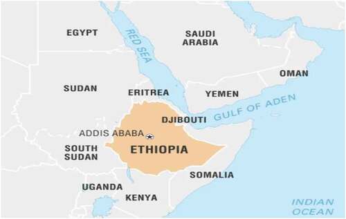
Ethiopia is one of least developed country located in the Horn of Africa, astronomically located at 8 00 N and 38 00 E (Figure 1). The population of Ethiopia is estimated in 2021 to be 117.8 million, and its capital city of Ethiopia is Addis Ababa, which serves as the capital of African countries and home of the African Union. Ethiopia is home to 54 ethnic groups and more than 80 languages. Its economy is built on agriculture. Coffee is a major export crop. Birr (ETB) serves as domestic currency for domestic exchange. Ethiopia’s Gross Domestic Product (GDP) was valued at 96.61 billion dollars in 2020.

Figure 1. Geographical map of Ethiopia and its neighboring countries.

3.2. Type and source of data

The research has employed secondary quantitative data to realize the defined study’s objective. Since the research entirely applies secondary data, data extraction is not as exhaustive as the primary data to collect and organize. The secondary data for both dependent variable (Real GDP) and explanatory variables, such as Labour force (LF), Gross Capital Formation (GCF), Education Expenditure (EDX), Health Expenditure (HEX), Total Government Expenditure (TGE), Secondary School Enrollment (SSE), Official Development Assistant (ODA) and Consumer Price Index (CPI) were acquired from concerned institutions and organizations. These institutions and organizations include the National Bank of Ethiopia (NBE), and World Economic Outlook (WEO) of IMF, the World Development Indicators (WDI) of the World Bank (WB), PES, CSA, and MoFED (Table 1). The summary of variables unit of measurements have been described in Table 2.

Table 1. Specific sources of data

S. No	Variables	Source of data
1	Real gross domestic product (RGDP)	NBE
2	Labour force (LF)	NBE and CSA
3	Gross capital formation (GCF	Planning and economic commission
4	Education expenditure (EDX)	MoE and WDI
5	Health expenditure (HEX)	MOFED
6	Total government expenditure (TGE)	NBE and MoFED
7	Secondary school enrollment (SSE)	MoE and EES
8	Official development assistant (ODA)	IMF
9	Consumer price index (CPI)	NBE

Table 2. Summary of variables’ description

Variables	Description	Unit of measurement
RGDP	Real Gross Domestic Product	The ratio changes in Real GDP
GCF	Gross Capita formation	The ratio of real gross capital formation to GDP
LF	Labor force	Labor force growth rate
EDX	Education expenditure	The ratio of government expenditure on education to GDP
HEX	Health expenditure	The ratio of government expenditure on health to GDP
SSE	Secondary school enrollment	Secondary school enrollment growth rate
TGE	Total government expenditure	The ratio of total government expenditure to GDP
ODA	Official development assistant	The ratio of official development assistants to GDP
CPI	Consumer price index	Price index

3.3. Data analysis

For data analysis, the study employed the inferential method of data analysis. The bound test of the ARDL model of the time series econometric method of data analysis was employed to evaluate the long-run and the short-run relationship between macroeconomic variables and human capital. In econometric procedures, the first unit root test was applied to check for the stationarity of the time series model employing the Augmented Dickey–Fuller (ADF) test and Phillips–Perron (PP) test. The co-integration test was applied using ARDL bound co-integration approach to examine whether the variables have a long-run relationship. The o-integration test serves as a bridge whether to specify both long-run and short-run models and the latter alone. If the bound test of co-integration leads to conclude the presence of a long-run relationship between the variables, both models should be estimated. The coefficients of the long-run model are estimated from a level form of the variables without differencing, but the short-run model (ECM) is derived from the ARDL model by transforming the equation into the re-parameterized form. The long-run information will not be lost in case the coefficient of error correction term captures evidence of the relationship through its speed of adjustment interpretation. However, the short-run version of the ARDL model is specified if the bound test does not indicate the existence of a long-run relationship (Nkoro & Uko, 2016).

A relatively simple participation is the importance of the augmented Solow human-capital-growth model. This model is an enhancement on the Solow growth model. The augmented Solow model applying the standard Cobb Douglas production function is hence specified as follows:

(1) ${\mathrm{Y}}_{\mathrm{t}}={\mathrm{K}}_{\mathrm{t}}^{\alpha }{\mathrm{H}}_{\mathrm{t}}^{\beta }{\left(\mathrm{A}\mathrm{L}\right)}^{1-\alpha -\beta }$(1)

Converting the equation to log-linear form:

(2) $\mathrm{l}\mathrm{n}{\mathrm{Y}}_{\mathrm{t}}=\alpha \mathrm{l}\mathrm{n}{\mathrm{H}}_{\mathrm{t}}+\beta \mathrm{l}\mathrm{n}{\mathrm{H}}_{\mathrm{t}}+\left(1-\alpha -\beta \right)ln\left(\mathrm{A}{\mathrm{L}}_{\mathrm{t}}\right)+\mathrm{V}$(2)

where, K is the level of physical capital, H is the level of Human Capital, L is the level of the labor force, A is level of Productivity/technology, Β is the Elasticity of Human capital for output, V is an error term, and α + β < 1.

The following empirically valuable log-linear form of the model is defined based on this theoretical framework (Mankiw et al., 1992). The autocorrelation between each variable was checked, and for those correlating with each other, they were dropped.

LnRGDP = f (LnLFt, LnGCFt, LnEDXt, LnHEXt, LnTGEt, LnSSE_t, LnODAt, LnCPIt, D₁, D₂) (3)

where LnRGDPt is the Natural logarithm of real GDP at time t, LnLFt is a Natural logarithm of labor force growth rate at time t, LnGCFt is the natural logarithm of gross capital formation at time t, LnEDXt is a Natural logarithm of education expenditure at time t, LnHEXt: a Natural logarithm of health expenditure at time t, LnTGEt: a Natural logarithm of total government expenditure at time t, LnSSEt: a Natural logarithm of secondary school enrollment at time t, LnODAt: a Natural logarithm of official development assistance at time t, LnCPIt: a Natural logarithm of consumer price index at time t, D₁: dummy variables for drought, and D₂ is the dummy variables for policy change.

3.4. Model specification

3.4.1. ARDL model

The study applied the autoregressive distributive lag (ARDL) model of the “Bounds Testing Approach” to co-integration which was used by (Pesaran et al., 2001). The model is selected based on the theoretically defined relationship between dependent and explanatory variables and the finite nature of the selected sample size. Given the endogenous variable, the ARDL approach of the co-integration testing procedure importantly helps us to understand whether the underlying variables in the model are co-integrated or not. Besides, the model is relatively efficient when the respondent is small or finite which is suitable for the chosen sample size. In addition, the researchers selected the ARDL procedure of co-integration method because of its several advantages. Firstly, the procedure can be used whether the regressors are I (1) or I (0), or a combination of both. Secondly, the ARDL model is statistically a stronger approach in determining the co-integration relationship between variables when the sample size is small, but other techniques like VAR models require large data samples for validity. Thirdly, the ARDL procedure does not restrict variables to have the same optimal lags as other models do. Moreover, endogeneity is less of a problem in this approach since each of the underlying variables in the model stands as a single equation. Fourth, the ARDL procedure can distinguish dependent and independent variables when there is a single long-run relationship that only a single reduced form of the equation is assumed in the model (Pesaran et al., 2001). Hence, the ARDL model becomes prevalent and appropriate for evaluating the long-run relationship and is extensively employed in empirical research. The study used Autoregressive Distributed Lag (ARDL) model to test the long-run co-integration relationships between variables. Therefore, the following ARDL approach is specified.

(4) $\mathrm{L}\mathrm{n}\mathrm{R}\mathrm{G}\mathrm{D}{\mathrm{P}}_{\mathrm{t}}={\beta }_0+{\lambda }_1\mathrm{L}\mathrm{n}\mathrm{R}\mathrm{G}\mathrm{D}{\mathrm{P}}_{\mathrm{t}-\mathrm{i}}+{\lambda }_2\mathrm{L}\mathrm{n}\mathrm{L}{\mathrm{F}}_{\mathrm{t}-\mathrm{i}}+{\lambda }_3\mathrm{L}\mathrm{n}\mathrm{G}\mathrm{C}{\mathrm{F}}_{\mathrm{t}-\mathrm{i}}+\hspace{0.17em}{\lambda }_4\mathrm{L}\mathrm{n}\mathrm{E}\mathrm{D}{\mathrm{X}}_{\mathrm{t}-\mathrm{i}}+{\lambda }_5\mathrm{L}\mathrm{n}\mathrm{H}\mathrm{E}{\mathrm{X}}_{\mathrm{t}-\mathrm{i}}+{\lambda }_6\mathrm{L}\mathrm{n}\mathrm{T}\mathrm{G}{\mathrm{E}}_{\begin{array}{c}t-i\end{array}}+{\lambda }_7\mathrm{L}\mathrm{n}\mathrm{S}\mathrm{S}{\mathrm{E}}_{\mathrm{t}-\mathrm{i}}+{\lambda }_8\mathrm{L}\mathrm{n}\mathrm{O}\mathrm{D}{\mathrm{A}}_{\mathrm{t}-\mathrm{i}}+{\lambda }_9\mathrm{L}\mathrm{n}\mathrm{C}\mathrm{P}{\mathrm{I}}_{\mathrm{t}-\mathrm{i}}+{\beta }_1\sum _{\mathrm{i}=0}^{\mathrm{n}}\mathrm{\Delta }\mathrm{L}\mathrm{n}\mathrm{R}\mathrm{G}\mathrm{D}{\mathrm{P}}_{\mathrm{t}-\mathrm{i}}+{\beta }_2\sum _{\mathrm{i}=0}^{\mathrm{n}}\mathrm{\Delta }\mathrm{L}\mathrm{n}\mathrm{L}{\mathrm{F}}_{\mathrm{t}-\mathrm{i}}+{\beta }_3\sum _{\mathrm{i}=0}^{\mathrm{n}}\mathrm{\Delta }\mathrm{L}\mathrm{n}\mathrm{G}\mathrm{C}{\mathrm{F}}_{\mathrm{t}-\mathrm{i}}+{\beta }_4\sum _{\mathrm{i}=0}^{\mathrm{n}}\mathrm{\Delta }\mathrm{L}\mathrm{n}\mathrm{E}\mathrm{D}{\mathrm{X}}_{\mathrm{t}-\mathrm{i}}+{\beta }_5\sum _{\mathrm{i}=0}^{\mathrm{n}}\mathrm{\Delta }\mathrm{L}\mathrm{n}\mathrm{H}\mathrm{E}{\mathrm{X}}_{\mathrm{t}-\mathrm{i}}+{\beta }_6\sum _{\mathrm{i}=0}^{\mathrm{n}}\mathrm{\Delta }\mathrm{L}\mathrm{n}\mathrm{T}\mathrm{G}{\mathrm{E}}_{\mathrm{t}-\mathrm{i}}+{\beta }_7\sum _{\mathrm{i}=0}^{\mathrm{n}}\mathrm{\Delta }\mathrm{L}\mathrm{n}\mathrm{S}\mathrm{S}{\mathrm{E}}_{\mathrm{t}-\mathrm{i}}+{\beta }_8\sum _{\mathrm{i}=0}^{\mathrm{n}}\mathrm{\Delta }\mathrm{L}\mathrm{n}\mathrm{O}\mathrm{D}{\mathrm{A}}_{\mathrm{t}-\mathrm{i}}+{\beta }_9\sum _{\mathrm{i}=0}^{\mathrm{n}}\mathrm{\Delta }\mathrm{L}\mathrm{n}\mathrm{C}\mathrm{P}{\mathrm{I}}_{\mathrm{t}-\mathrm{i}}+{\beta }_{10}{\mathrm{D}}_1+{\beta }_{11}{\mathrm{D}}_2+{\mathrm{e}}_{\tau }t$(4)

Where LnGDPt is the Natural logarithm of real GDP at time t, LnLFt is a Natural logarithm of labor force growth rate at time t, LnGCFt is the natural logarithm of gross capital formation at time t, LnEDXt is a Natural logarithm of education expenditure at time t, LnHEXt is a Natural logarithm of health expenditure at time t, LnTGEt is a Natural logarithm of total government expenditure at time t, LnSSEt is a Natural logarithm of secondary school enrollment at time t, LnODAt is a Natural logarithm of official development assistance at time t, LnCPIt is a Natural logarithm of consumer price index at time t, D₁ is dummy variables for drought, and D₂ is dummy variables for policy change.

The coefficients measuring long-run relationships are λ1, λ2, λ3, λ4, λ5, λ6, λ7, λ8, and λ9. The coefficients measuring short-run relationships are β1, β2, β3, β4, β5, β6, β7, β8, β9, β10, and β11, n is the lag length of the autoregressive process, and et is an error term.

Therefore, the following long-run stable model was calculated after verifying a long-run relationship between the variables.

(5) $\mathrm{L}\mathrm{n}\mathrm{R}\mathrm{G}\mathrm{D}{\mathrm{P}}_{\mathrm{t}}={\beta }_0+{\beta }_1\sum _{\mathrm{i}=0}^{\mathrm{n}}\mathrm{L}\mathrm{n}\mathrm{R}\mathrm{G}\mathrm{D}{\mathrm{P}}_{\mathrm{t}-\mathrm{i}}+{\beta }_2\sum _{\mathrm{i}=0}^{\mathrm{n}}\mathrm{L}\mathrm{n}\mathrm{L}{\mathrm{F}}_{\mathrm{t}-\mathrm{i}}+{\beta }_3\sum _{\mathrm{i}=0}^{\mathrm{n}}\mathrm{L}\mathrm{n}\mathrm{G}\mathrm{C}{\mathrm{F}}_{\mathrm{t}-\mathrm{i}}+{\beta }_4\sum _{\mathrm{i}=0}^{\mathrm{n}}\mathrm{L}\mathrm{n}\mathrm{E}\mathrm{D}{\mathrm{X}}_{\mathrm{t}-\mathrm{i}}+{\beta }_5\sum _{\mathrm{i}=0}^{\mathrm{n}}\mathrm{L}\mathrm{n}\mathrm{H}\mathrm{E}{\mathrm{X}}_{\mathrm{t}-\mathrm{i}}+{\beta }_6\sum _{\mathrm{i}=0}^{\mathrm{n}}\mathrm{L}\mathrm{n}\mathrm{T}\mathrm{G}{\mathrm{E}}_{\mathrm{t}-\mathrm{i}}+{\beta }_7\sum _{\mathrm{i}=0}^{\mathrm{n}}\mathrm{L}\mathrm{n}\mathrm{S}\mathrm{S}{\mathrm{E}}_{\mathrm{t}-\mathrm{i}}+{\beta }_8\sum _{\mathrm{i}=0}^{\mathrm{n}}\mathrm{L}\mathrm{n}\mathrm{O}\mathrm{D}{\mathrm{A}}_{\mathrm{t}-\mathrm{i}}+{\beta }_9\sum _{\mathrm{i}=0}^{\mathrm{n}}\mathrm{L}\mathrm{n}\mathrm{C}\mathrm{P}{\mathrm{I}}_{\mathrm{t}-\mathrm{i}}+{\beta }_{10}{\mathrm{D}}_1+{\beta }_{11}{\mathrm{D}}_2+{\mathrm{v}}_{\mathrm{t}}\hspace{0.17em}$(5)

To estimate the vector error correction model that reveals the dynamic short-run parameters. The standard ECM is estimated as follows:

(6) $\mathrm{\Delta }\mathrm{L}\mathrm{n}\mathrm{R}\mathrm{G}\mathrm{D}{\mathrm{P}}_{\mathrm{t}}={\beta }_0+{\beta }_1\sum _{\mathrm{i}=0}^{\mathrm{a}}\mathrm{L}\mathrm{n}\mathrm{R}\mathrm{G}\mathrm{D}{\mathrm{P}}_{\mathrm{t}-\mathrm{i}}+{\beta }_2\sum _{\mathrm{i}=0}^{\mathrm{b}}\mathrm{L}\mathrm{n}\mathrm{L}{\mathrm{F}}_{\mathrm{t}-\mathrm{i}}+{\beta }_3\sum _{\mathrm{i}=0}^{\mathrm{c}}\mathrm{\Delta }\mathrm{L}\mathrm{n}\mathrm{G}\mathrm{C}{\mathrm{F}}_{\mathrm{t}-\mathrm{i}}+{\beta }_4\sum _{\mathrm{i}=0}^{\mathrm{d}}\mathrm{\Delta }\mathrm{L}\mathrm{n}\mathrm{E}\mathrm{D}{\mathrm{X}}_{\mathrm{t}-\mathrm{i}}+{\beta }_5\sum _{\mathrm{i}=0}^{\mathrm{e}}\mathrm{\Delta }\mathrm{L}\mathrm{n}\mathrm{H}\mathrm{E}{\mathrm{X}}_{\mathrm{t}-\mathrm{i}}+{\beta }_6\sum _{\mathrm{i}=0}^{\mathrm{f}}\mathrm{\Delta }\mathrm{L}\mathrm{n}\mathrm{T}\mathrm{G}{\mathrm{E}}_{\mathrm{t}-\mathrm{i}}+{\beta }_7\sum _{\mathrm{i}=0}^{\mathrm{g}}\mathrm{\Delta }\mathrm{L}\mathrm{n}\mathrm{S}\mathrm{S}{\mathrm{E}}_{\mathrm{t}-\mathrm{i}}+{\beta }_8\sum _{\mathrm{i}=0}^{\mathrm{h}}\mathrm{\Delta }\mathrm{L}\mathrm{n}\mathrm{O}\mathrm{D}{\mathrm{A}}_{\mathrm{t}-\mathrm{i}}{\beta }_9\sum _{\mathrm{i}=0}^{\mathrm{h}}\mathrm{\Delta }\mathrm{L}\mathrm{n}\mathrm{C}\mathrm{P}{\mathrm{I}}_{\mathrm{t}-\mathrm{i}}+{\beta }_{10}{\mathrm{D}}_1+{\beta }_{11}{\mathrm{D}}_2+\delta \mathrm{E}\mathrm{C}{\mathrm{T}}_{\mathrm{t}-1}+{\mathrm{U}}_{\mathrm{t}}$(6)

Where: β₁, β₂, β₃, β₄, β₅, β₆, β₇, β_8, β₉, β_10, and β₁₁ are coefficients that represent the short-run dynamics of the model. It is a vector of white noise error terms, and (a − h) presents the maximum lag length of each variable in the autoregressive process. The dummy variables for recurrent drought and policy change are D₁ and D₂. ECT is the error correction term with one period lag; δ is a parameter of error correction that evaluates the adjustment speed towards the long-run equilibrium.

The error correction term (ECT) measures the relationship between the short-run and the long-run. It is developed from the long-run model and shows how variables quickly converge to equilibrium. The coefficient of ECT should also be statistically significant. If the coefficient has a negative sign, it confirms the presence of a co-integrating relationship; however, if the sign of the coefficient is positive, the model is explosive that there is no convergence. If the estimates of ECT = 1, then 100% of the adjustment takes place within the period, the adjustment is rapid and complete, and if the estimate of ECT = 0.5, then 50% of the adjustment takes place each year. ECT = 0, indicates non-existence of adjustment.

4. Results and discussions

4.1. Data overview and descriptive analysis

4.1.1. Expenditure on education and health in Ethiopia

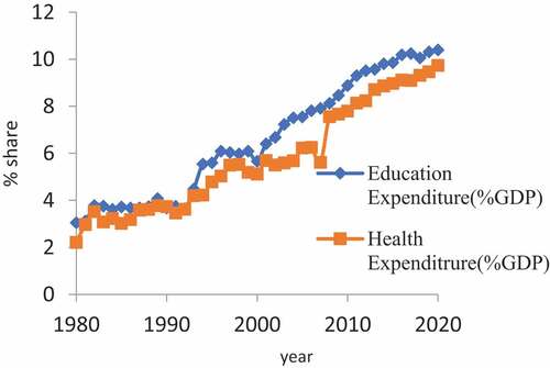
Figure 2 presents the share of total expenditure on education to GDP slightly enhances from a mean of 2.51% in the years 1980–1982 to an average of 3.65% in 1982–1992. During 1992–1998, the share has also enhanced to a mean value of 4.5%. Between 2000 and 2006, the mean share of total expenditure on education to GDP was 5.66%. After, it has enhanced from a mean of 7.56% in the years 2007–2010 to an average of 9.13% in the year 2010–2020. This study is in line with the study of (Kaj et al., 2010)

Figure 2. Trends in the share of government expenditure on education and health to GDP in Ethiopia.

Source: Own calculation based on MoFED (2021)

4.1.2. Real GDP and its trend in Ethiopia

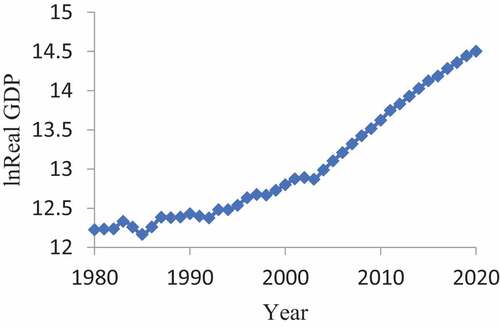
Trends of Real GDP present the change in the Real GDP over the years. Therefore, it is focusing to note that growth trends are highly not regular (Figure 3). Agricultural sector performance, which is related to the differences of nature, could be one reason for such not regularities. In addition, continuous war and instabilities in the country are the other factors responsible for such a collapsed economic trend (Tadesse, 2011).

Figure 3. Trends of Real GDP in Ethiopia (1980–2020).

Source: Own calculation based on National Bank of Ethiopia data (2020)

4.1.3. Labor force growth rate

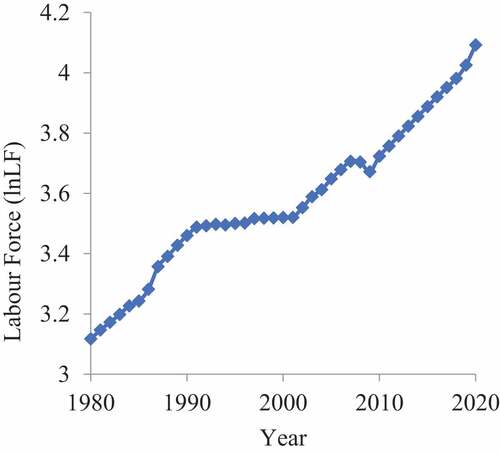
The labor force growth rate is the various people available to job or work as a percentage of the total population. The rate enhanced between 1980 and 1991 from 3.12 in 1980 to 4.89 in 1991 and then after that it is almost constant at an average rate of 3.5 until 2000. After 2000, the rate increases continuously and reaches 3.7 in 2006. As present in Figure 4, the labor adoption rate starts to decline to reach 3.67 in a year 2006 to 2009 due to the lowered financial crisis. After 2009, the participation rate showed 4.09 in 2020. This study is similar to the study (Kidanemariam, 2014; Tadesse, 2011).

Figure 4. Trends of Labor force growth rate in Ethiopia.

Source: Own calculation based on NBE and CSA, 2021

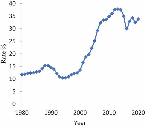
4.1.4. Secondary school enrollment rate

From 1985 to 1988, the secondary school gross enrollment rate increased from 11.23% to 15.06%. As shown in Figure 5, the gross enrolment ratio in secondary education for Ethiopia was 35.2% in 2015. The total enrolment ratio in secondary education in Ethiopia increased from 12.2% to 35.2% in 1992 with growth at an average annual rate of 6.06% in 2015 (Tadesse, 2011).

Figure 5. Trends of secondary school enrolment rate in Ethiopia (1980–2020).

Source: Own calculation from MoE and EES (2021) database

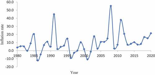
4.1.5. Inflation and its trend in Ethiopia

Trend inflation is commonly described as a common factor taken from observed inflation rates after removing cyclical impacts from economic cycles and other transient distortions. The average inflation rate in Ethiopia by 2020 amounted to about 20.35% compared to the previous year. According to the trend illustrated by actual data and the IMF (2018) report, the country has been experiencing growing price levels since 2003. The General inflation rate was negative in 1996 and 2001 with the value of 8.9% and 10.8%, respectively. However, the general inflation rate amplified to 17.7% in 2003 and then went down in 2004 to 2.4% due to agricultural output recovery and better economic growth performance. Between 2004 and 2008, inflation has been growing at a rising rate. In 2008, general inflation rates surged to 55.51% & 78.28%, respectively. In contrast, Figure 6, from international institutions show that Ethiopia’s general CPI rise is 44.38%, even though the trend is the highest for both databases. According to (Le et al., 2003), high inflation during this period was caused by a combination of an agricultural supply shock, money growth, and imported inflation caused by foreign prices. From 1981 to 2013, the distinctive character of the inflation pattern of increase and decline was observed. In 2009/10, it was reduced to 2.7%, and then to 8% in 2010. In 2011 and 2012, the rate increased to 38% and 20.8%, respectively. From 2012 to 2016, however, general inflation has been in the single digits. The pattern then flipped in 2017, when inflation began to rise in double digits until the end of the study period (2020), with growth rates of 10.7% and 21.5% in these years, respectively.

Figure 6. Inflation annual percentage change trend, Ethiopia (1980–2020).

Source: own computation from NBE data, 2021

4.2. Lag length selection

Before undertaking unit, root tests and estimating the underlying model, maximum lags length must be determined at an early stage. Because the estimation results are highly sensitive to the lag length of variables, the optimum number of lags needs to be selected before conducting other tests or estimations (Mallik, 2008). These lag numbers are selected by information criteria: Likelihood Ration (LR), Akaike Information Criterion (AIC), Schwartz-Bayesian Information Criterion (SC), final prediction error (FPE), Hannan-Quinn information criterion (HQIC). These criteria automatically select the maximum lag length of variables to be incorporated into the specified model, but they may not necessarily give the same result due to their applicability in different sample sizes. For example, AIC and FPE are appropriate for small sample sizes (60 or less), while SC and HQIC better perform for large (greater than 60) sample sizes. This study, therefore, used AIC due to its better performance compared to other information criteria when a relatively small sample size is applied, i.e., n < 60 observations. The next table shows the computed result using EViews 10.

From Table 3, the asterisks (*) mark the maximum lag length automatically selected by the criteria. Accordingly, all criteria except SC indicated that the optimum lag that minimizes their corresponding values is two. However, we should note that it does not necessarily mean each variable has two lag lengths. It rather shows the maximum lengths above which lag (s) should not be included. Thus, some variables can have lag lengths lower than the automatically determined ones. For example, when each of them is tested individually, the dummy variable and logarithmic form of other variables—RGDP, EDX, TGE, SSE, ODA, and CPI—have one maximum lag length, while the rest explanatory variables have two. These findings are in line with those (Mallik, 2008).

Table 3. Lag order selection

Lag	LogL	LR	FPE	AIC	SC	HQ
0	−141.8175	NA	7.02e-11	7.836796	8.306006	8.005145
1	205.3712	480.7229	8.07e-16	−3.762626	1.867891*	−1.742445
2	400.4398	160.0563*	9.89e-17*	−7.561017*	3.230806	−3.689004*

Note: * Indicates lag order selected by the criterion

4.3. Unit root test

Lag length determination is followed by conducting a stationarity test. It is a pre-requisite for the co-integration test of the time-series variables because estimation without undertaking the unit root test may lead to spurious results. This test is also essential to make sure that all variables are integrated of order zero or one so that the method ARDL bound test will not be hindered. The Augmented Dickey–Fuller (ADF) and the Phillips–Perron (PP) unit root testing methods were employed for this purpose. In the ADF test, the Akaike information criterion (AIC) was selected because the lag length of the time series was determined based on this criterion due to its good performance in a small finite sample size. Besides, Newey–West bandwidth automatically selects lag for Phillips–Perron (PP) unit root test. Next, Table 4 summarizes the results of the stationary test from both methods (Pesaran et al., 2001).

Table 4. Augmented Dickey-Fuller and Phillips-Perron Unit Root Tests

At level				At first difference
Series	Intercept	Intercept & trend	Intercept	Intercept & trend
		ADF unit	root test
LnRGDP	2.071	−0.930	−5.18***	−6.23***
LnGCF	1.27	−1.64	−7.42***	−7.92**
LnLF	0.65	−1.09	−3.28***	−3.31***
LnODA	−0.33	−3.31	−7.44***	−5.77***
LnTGE	0.87	−1.52	−5.49***	−5.92***
LnHEX	0.92	−2.96	−8.03***	−8.02***
LnEDX	−0.11	−2.35	−5.97***	−5.88***
LnSSE	−0.024	−1.53	−5.19***	−5.19***
LnCPI	1.91	−0.67	−4.71***	−5.21***
D1	−6.64	−6.61	−6.49**	−6.38***
D2	−5.72*	−5.74	−8.63***	−8.52***
			Philips-Perron
LnRGDP	2.21	−0.880	−5.32***	−6.24***
LnGCF	2.04	−1.34	−7.40***	−14.56**
LnLF	0.38	−1.14	−3.27***	−3.30***
LnODA	−3.30	−3.35	−7.66**	−7.76***
LnTGE	1.74	−1.34	−6.19***	−7.36***
LnHEXP	−0.05	−2.57	−8.40***	−8.78***
LnEDEXP	−0.12	−2.43	−5.98***	−5.90***
LnSSE	−0.28	−1.79	−5.37***	−5.37***
LnCPI	1.68	−0.86	−4.73***	−5.17***
D1	−22.19	−24.12	−39.58**	−39.81***
D1	−6.69	−8.55	−24.14***	−24.19***

Source: Author computation based on the result of EViews 10 computation

Note: The values represent t-statistics of the ADF (upper panel) and PP (lower panel) unit root tests. The asterisks ***, **, and * denote the statistical significance of the test at 1, 5, and 10 percent levels of significance respectively.

The ADF and Phillips-Perron (PP) unit root tests result reveals that all variables except policy change (D2), which is stationary under the ADF unit root test with an intercept at a 10% level of significance are non-stationary at the level. From the PPF test that all variables become stationary at least at a 5% significance level for both intercept and intercept & trend situations after the first difference. These findings show that nine variables are I (1), and one is I (2), with intercept and trend (0). Such findings of the stationarity test would not allow us to employ the Johansen approach of co-integration. This is one of the critical motivations for employing ARDL methodology (bounds test methodology of co-integration; Pesaran et al., 2001).

4.4. Co-integration test and the ARDL long-run model

After running the ARDL model, a co-integration test is required to identify whether to specify either long-run and short-run models or the latter alone. To check the presence of co-integration in the ARDL model (Pesaran et al., 2001) developed the bound test, which was later improved for small sample sizes. Having lower and upper values, the bound test depends on F-statistics. The value of F-statistics is computed using Wald-test from the null hypothesis by making long-run coefficients equal to zero. If the computed F-statistics lies below the lower bound, the null hypothesis of no co-integration will be failed to be rejected. Contrarily, if the value is greater than the upper bound of the statistics, the null hypothesis of no co-integration is rejected in the conclusion of the existence of a long-run relationship (Tadesse, 2011). The following table presents the result from the bound test.

F-statistics from above Table 5 reveals that the F-value (4.16) exceeds the values of the upper bound at all levels of significance. Therefore, we can reject the null hypothesis of no level relationship in favor of the alternative hypothesis, supporting the existence of co-integration. This evidence robustly confirms the presence of a long-run relationship between dependent and right-hand variables. Hence, long-run and short-run models can be reasonably estimated. The following table reports the estimated parameters’ estimates of the long-run equation of the model (Mallik, 2008).

Table 5. ARDL Bound test for Long-run relationship

F-Bounds Test		Null Hypothesis: No levels of relationship
Test Statistic	Value	Level of Significance.	I (0)		I (1)
			Asymptotic: n = 1000
F-statistic	4.161872	10%	1.83		2.94
K	10	5%	2.06		3.24
		2.5%	2.28		3.5
		1%	2.54		3.86

Source: Own computation using EViews 10

Table 6 presents the long-run result of the ARDL model with the real gross domestic product (LNRGDP) as a dependent variable whereas the rest variables: labor force (LNLF), gross capital formation (LNGCF), education expenditure (LNEDX), health expenditure (LNHEX), total government expenditure (LNTGE), secondary school enrollment (LNSSE), official development assistant (LNODA), consumer price index (LNCPI), drought (D1) and policy change (D2) are explanatory variables. As indicated in the preceding section, all variables are expressed in logarithm form except dummy variables. The last variable (DUM) takes one (1) artificial number for the policy change from 1980 to 2020 and zero (0) otherwise. Thus, we do not need to express the last two variables in logarithm form. Overall, the incorporated regressors explained the model by 99.9% of the variation. In the long run, the labor force (LNLF), total government expenditure (LNTGE), and drought dummy (D₁) are not statistically significant. Gross capital formation (LNGCF), secondary school enrolment (LNSSE), and consumer price index (LNCPI) are positive and found to be highly significant at a 1% level of significance. In addition, education expenditure (LNEDX), health expenditure (LNHEX), and policy change (D₂) are positive and significant at 5%. On the other hand, the official development assistant (LNODA) is negative and significant at 5%.

Table 6. The long-run ARDL parameter estimates

Variable	Coefficient	Std. Error	t-Statistic	Prob.
LNLF	0.213836	0.139033	1.538021	0.1424
LNGCF	0.341793	0.041216	8.292720	0.0000***
LNEDX	0.076883	0.031692	2.425922	0.0267**
LNHEX	0.087692	0.056267	1.558506	0.0375**
LNTGE	−0.023153	0.039738	−0.582653	0.5678
LNSSE	0.018406	0.002784	6.611950	0.0000***
LNODA	−0.059858	0.023822	−2.512720	0.0224**
LNCPI	0.274811	0.082891	3.315335	0.0041***
D1	−0.014811	0.020473	−0.723423	0.4793
D2	0.068543	0.032472	2.110818	0.0499**
C	6.168178	1.402220	4.398866	0.0004***
R-squared	0.999061	Mean dependent var	11.07910
Adjusted R-squared	0.997901	S.D. dependent var	0.722231
S.E. of regression	0.033087	Akaike info criterion	−3.681490
Sum squared resid	0.018611	Schwarz criterion	−2.743071
Log-likelihood	93.78906	Hannan-Quinn criteria	−3.344794
F-statistic	861.3726	Durbin-Watson stat	2.272350
Prob(F-statistic)	0.000000

*Note: P-values and any subsequent tests do not account for model selection.

Source: Own computation using EViews 10, 2021

Notes: The sample period used for estimation is 1980–2020. The asterisks ***, **, and * mark the statistical significance of coefficients at 1, 5, and 10 percent levels of significance, respectively

4.5. Post estimation diagnostics and stability tests

The post estimation tests are required to check the reliability of the estimated result. The most commonly used tests in dynamic models are normality, autocorrelation, heteroscedasticity, model specification, and stability tests. Such tests are undertaken to guarantee regression of the model that the obtained results are free from spurious regression. Moreover, they warrant the robustness of the model (Mallik, 2008).

As we can see, from Table 7, the model passed all post-estimation diagnostic tests. The Breusch-Godfrey Lagrange Multiplier autocorrelation test fails to reject the null hypothesis of no residual autocorrelation at a 5% level of significance. In addition, Durbin–Watson’s d-statistics lies between 1.7 and 2.3, which supports the evidence from the Breusch-Godfrey LM test. The d-statistics also confirms the non-spuriousness of the regression since its value exceeds the adjusted R-squared. To check the heteroscedasticity problem, the conducted Breusch–Pagan–Godfrey test conveys that both standard (0.43) and Chi-squared probability (0.38) values are greater than the 5% level of significance. This result leads to accepting the null hypothesis stating the homoscedastic nature of the error variance. At F (1, 36) degrees of freedom, both standard (0.51) and Chi-squared (0.50) probabilities of the ARCH test support robustness of the result from the Breusch–Pagan–Godfrey test. Hence, the result supports the absence of the heteroscedasticity problem. Furthermore, the above summary table on diagnostics tests confirms the normality of the residuals and the correct specification of the model. JB statistics (0.72) is much higher than the standard level of significance (0.05). Since the residuals are normally distributed, we can claim that the hypotheses of the coefficients’ estimates are validly tested. Besides, the model specification test checked by the Ramsey RESET test shows the absence of omitted variable (s) because the RESET test p-value (0.29) highly exceeds the standard significance level. Therefore, this evidence leads us to conclude that the model is correctly specified and the result is robust as well (Alam et al., 2022; Mahmood & Murshed, 2020).

Table 7. Summary of diagnostics tests

Types of tests	F-statistics	Df	Prob.	Prob. Chi-Square
Breusch-Godfrey test	2.87	F (2,15)	0.0877	0.0645
Heteroskedasticity (BPG)	1.083605	F (21,17)	0.4383	0.3811
Heteroskedasticity (ARCH)	0.434389	F (1,36)	0.5140	0.5009
Normality test (JB-statistics)	0.63		0.72
Ramsey RESET Test	1.186353	(1, 16)	0.2922
Durbin-Watson test	2.27 (d-stat)

Source: Compiled from diagnostics tests after ARDL model estimation using EViews 10, 2021

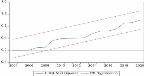
4.6. Model stability test

The most commonly used to test the stability of a model are the cumulative sum of recursive (CUSUM) test and CUSUM of squares graph. The tests are based on the residuals from the recursive estimates and are presented in the figure.

Null hypothesis H₀: CUSUM distribution is symmetrically centered at 0.

Alternative hypothesis H₁: CUSUM is not symmetrically distributed.

Decision rule: The null hypothesis of the normal distribution is failed to be rejected when the graph of CUSUM statistics lies within the bounds of the critical region at a 5% level of significance and the alternative hypothesis of not symmetrically distributed is accepted otherwise.

From Figure 7, we fail to reject the null hypothesis that the cumulative sum of squares of recursive (CUSUM) is symmetrically distributed. At the same level of significance, the CUSUM test also confirms a similar result, supporting the robust stability of the model. Since the model passed all diagnostic and stability tests, we can proceed to examine the co-integration test (Alam et al., 2022).

Figure 7. CUSUM of Squares.

Source: Model diagnostics test result using EViews 10

4.7. The short-run ARDL model estimation result

Estimating an error correction model would be imperative once the presence of a long-run relationship between the variables is confirmed by the co-integration test. The re-parameterized short-run relationship between dependent and independent variables was scrutinized with the Error Correction Model (ECM; Nkoro & Uko, 2016). The following Table 8 reports regression results obtained from ARDL-error correction model.

Table 8. ECM Regression

Variable	Coefficient	Std. Error		t-Statistic	Prob.
C	6.168178	0.721084		8.554031	0.0000***
D(LNGCF)	0.064973	0.024677		2.632922	0.0174**
D (LNGCF (−1))	−0.187491	0.040788		−4.596668	0.0003***
D(LNHEX)	−0.012495	0.012768		−0.978635	0.3415
D (LNHEX (−1))	0.026239	0.013610		1.927873	0.0707*
D(LNSSE)	0.006373	0.002735		2.330218	0.0324**
D (LNSSE (−1))	−0.012243	0.003850		−3.179814	0.0055***
D(LNODA)	−0.018337	0.009722		−1.886114	0.0765*
D(LNCPI)	−0.013965	0.058662		−0.238053	0.8147
D (LNCPI (−1))	−0.473676	0.093163		−5.084405	0.0001***
D(D2)	0.024881	0.008829		2.818129	0.0118**
CointEq (−1) *	−0.952854	0.111745		−8.527036	0.0000***
R-squared	0.861643	Mean dependent var			0.056578
Adjusted R-squared	0.805276	S.D. dependent var			0.059496
S.E. of regression	0.026254	Akaike info criterion			−4.194311
Sum squared resid	0.018611	Schwarz criterion			−3.682446
Log-likelihood	93.78906	Hannan-Quinn criteria			−4.010658
F-statistic	15.28614	Durbin-Watson stat			2.272350
Prob(F-statistic)	0.000000

Sources: own computation using EViews 10

The dependent variable is DCPIt over the sample period 1981–2020. The asterisks ***, **, and * mark the statistical significance of coefficients at 1, 5, and 10 percent levels of significance, respectively.

The error correction coefficient in the short-term analysis is −0.9528, implying an annual adjustment of about 95.28% to the long-term equilibrium. When secondary school enrollment enhances by 1%, real GDP enhances by 0.006373. Health has no statistically significant effect on the Ethiopian economy in the short run. When health spending increases by 1%, real GDP increases by 0.02623.

In the long run, gross capital formation, followed by health human capital and education human capital, are the main contributors to real GDP growth. In other words, the results show that the share of health expenditure, the share of education expenditure, and the secondary school enrolment rate significantly increase economic performance. Holding other factors constant, a 1% change in health status leads to a 0.088% change in real GDP. In addition to health status, the level of education has a statistically significant long-term effect on the Ethiopian economy. A 1% increase in education expenditure and secondary school enrolment leads to a 0.077% and 0.02% change in real GDP, respectively. Official development assistance, on the other hand, hurts the economy. The results of this study on long-term analysis have a positive impact on education and human capital for health.

5. Conclusion

This study was aiming to analyze the human capital and its impact on Ethiopian economic growth applying real GDP as a proxy for economic growth. To evaluate the impact of human capital on Ethiopian economic growth (real GDP), the study has applied the ARDL model to co-integration and the error correction model (ECM). The main conclusion is that in the long run, gross capital formation followed by human health capital and human education capital are the most important contributors to the rise in Real GDP. In other words, the results show that as the ratio of expenditure on health services, the ratio of education expenditure, and secondary school enrolment rises economic performance dramatically. Keeping other things being constant, the 1% change in health brought a 0.088% change in real GDP. Next to health status, education level has a statistically significant long-run impact on the Ethiopian economy. 1% increase in education expenditure and secondary school enrolment has presented in 0.077% and 0.02% change in real GDP, respectively. However, Official development assistance hurts the economy. Consumer price index (CPI) and policy change have a positive impact on Ethiopian economic growth. The results of this study concerning the long-run analysis have a positive impact on education, and human health capital. The coefficient of error correction term in the short-run analysis is −0.9528, indicating about 95.28% yearly adjustment towards long-run equilibrium. When secondary school enrollment enhances by 1%, real GDP enhances by 0.006373. Health status has no statistically significant short-run impact on the Ethiopian economy. When health expenditure enhances by 1%, real GDP enhances by 0.026239. In the short run, policy change is also positively significant effect on the Ethiopian economic growth. Like its negative long-run effect, official development assistance has a significant effect on the economy in the short run. Consumer Price Index at one period lag has a negatively significant effect on the Ethiopian economic growth. Therefore, this study shows that there is a long-run and short-run impact of human capital on the economic growth of Ethiopia.

Acknowledgement

The authors would like to extend their gratitude to the Jimma University, College of Business and Economics, National Bank of Ethiopia (NBE), Central Statistical Authority (CSA), Planning and economic commission, MOFED, MoE, WDI, EES, IMF, and Jimma University staff for the secondary data and unreserved support they provided to the successful accomplishment of the study.

Disclosure statement

No potential conflict of interest was reported by the author(s).

Additional information

Funding

The authors received no direct funding for this research.

References

- Ahmed, Z., Nathaniel, S. P., & Shahbaz, M. (2021). The criticality of information and communication technology and human capital in environmental sustainability: Evidence from Latin American and Caribbean countries. Journal of Cleaner Production, 286, 125529. https://doi.org/10.1016/j.jclepro.2020.125529
- Ahmed, Z., & Wang, Z. (2019). Investigating the impact of human capital on the ecological footprint in India: An empirical analysis. Environmental Science and Pollution Research, 26(26), 26782–18. https://doi.org/10.1007/s11356-019-05911-7
- Alam, N., Hashmi, N. I., Jamil, S. A., Murshed, M., Mahmood, H., & Alam, S. (2022). The marginal effects of economic growth, financial development, and low-carbon energy use on carbon footprints in Oman: Fresh evidence from autoregressive distributed lag model analysis. Environmental Science and Pollution Research, 29(50), 76432–76445. https://doi.org/10.1007/s11356-022-21211-z
- Barro, R. J. (2003). Determinants of economic growth in a panel of countries. Annals of Economics and Finance, 4, 231–274.
- Bezabih, B. (2018). The impact of human capital on economic growth in Ethiopia: Evidence from Johansen co-integration approach. http://repository.smuc.edu.et/bitstream/123456789/3946/1/Thesis%20Final.pdf
- Borojo, D. G., & Yushi, J. (2015). The impact of human capital on economic growth in Ethiopia. Journal of Economics and Sustainable Development, 6(16), 109–118. https://core.ac.uk/download/pdf/234647202.pdf
- Dawud, S. A. (2020). The impact of human capital development on economic growth in Ethiopia. American Journal of Theoretical and Applied Business, 6(4), 47. https://doi.org/10.11648/j.ajtab.20200604.11
- Folloni, G., & Vittadini, G. (2010). HUMAN CAPITAL MEASUREMENT: A SURVEY. Journal of Economic Surveys, 24(2), 248–279. https://doi.org/10.1111/j.1467-6419.2009.00614.x
- Gebrehiwot, K. G. (2016). The impact of human capital development on economic growth in Ethiopia: Evidence from ARDL approach to co-integration. Bahir Dar Journal of Education, 16, 1. https://core.ac.uk/download/pdf/234647132.pdf
- Kaj, G., Fadi, F., & Rahnama, M. (2010). The effects of foreign aid on economic growth in developing countries. The Journal of Developing Areas 51.3 (2017): 153-171. College of Business, Tennessee State University.
- Kidanemariam, G. (2014). The impact of human capital development on economic growth in Ethiopia: Evidence from ARDL approach to co-integration. A Peer-Reviewed Indexed International Journal of Humanities & Social Science, 2, 64–88. https://doi.org/10.11648/j.ajtab.20200604.11
- Le, T., Gibson, J., & Oxley, L. (2003). Cost- and income-based measures of human capital. Journal of Economic Surveys, 17(3), 271–307. https://doi.org/10.1111/1467-6419.00196
- Loehwing, W. F. (1948). The developmental physiology of seed plants. Science (New York, N.Y.), 107(2786), 529–533. https://doi.org/10.1126/science.107.2786.529
- Mahmood, H., & Murshed, M. (2020). OIL PRICE AND ECONOMIC GROWTH NEXUS IN SAUDI ARABIA: ASYMMETRY ANALYSIS. International Journal of Energy Economics and Policy, 11(1), 29–33. https://doi.org/10.32479/ijeep.10382
- Mallik, G. (2008). Foreign Aid and economic growth: A cointegration analysis of the six poorest African countries. Economic Analysis and Policy, 38(2), 2. https://doi.org/10.1016/S0313-5926(08)50020-8
- Mankiw, N. G., Romer, D., & Weil, D. N. (1992). A contribution to the empirics of economic growth. The Quarterly Journal of Economics, 107(2), 407–437. https://doi.org/10.2307/2118477
- Marimuthu, M., Lawrence, A., & Maimunah, I. (2009). Human capital development and its impact on firm performance: Evidence from developmental economics, 2(8), 60–67. http://www.sosyalarastirmalar.com/cilt2/sayi8pdf/marimuthu_arokiasamy_ismail.pdf
- Narayan, P. K. (2005). The saving and investment nexus for China: Evidence from cointegration tests. Applied Economics, 37(17), 1979–1990. https://doi.org/10.1080/00036840500278103
- Nkoro, E., & Uko, A. K. (2016). Autoregressive Distributed Lag (ARDL) cointegration technique: Application and interpretation. Journal of Statistical and Econometric Methods, 5(4), 63–91. https://ideas.repec.org/a/spt/stecon/v5y2016i4f5_4_3.html
- Odior, E. S. O. (2011). Government expenditure on health, economic growth and long waves in A CGE micro-simulation analysis: The case of Nigeria. European Journal of Economics, Finance and Administrative Sciences.
- Pesaran, M. H., Shin, Y., & Smith, R. J. (2001). Bounds testing approaches to the analysis of level relationships. Journal of Applied Econometrics, 16(3), 289–326. https://doi.org/10.1002/jae.616
- Siraj, T. (2012). Official development assistance (ODA), public spending and economic growth in Ethiopia. Journal of Economics and International Finance, 4, 8. https://doi.org/10.5897/JEIF11.142
- Sisodia, G., Jadiyappa, N., & Joseph, A. (2021). The relationship between human capital and firm value: Evidence from Indian firms. Cogent Economics & Finance, 9(1), 1954317. https://doi.org/10.1080/23322039.2021.1954317
- Tadesse, T. (2011). Foreign aid and economic growth in Ethiopia: A cointegration analysis. The Economic Research Guardian, 1(2), 88–108. https://ideas.repec.org/a/wei/journl/v1y2011i2p88-108.html
- Tolasa, S., Tolla Whakeshum, S., & Mulatu, N. T. (2022). Macroeconomic determinants of inflation in Ethiopia: ARDL approach to cointegration. European Journal of Business Science and Technology, 8(1), 96–120. https://doi.org/10.11118/ejobsat.2022.004
- Umaru, A. (2011). Human capital: Education and health in economic growth and development of the Nigerian economy. British Journal of Economics, 2, 1. http://www.ajournal.co.uk/EFpdfs/EFvolume2(1)/EFVol.2%20(1)%20Article%203.pdf