Modelling asymmetric sovereign bond yield volatility with univariate GARCH models: Evidence from India

Abstract

Does Indian sovereign yield volatility reflect economic fundamentals, or whether it is a self-generated force flowing through markets with little connection to such fundamentals? To answer the question, this research explores the volatility dynamics and measures the persistence of shocks to the sovereign bond yield volatility in India from 1 January 2016, to 18 May 2022, using a family of GARCH models. The empirical results indicate the high volatility persistence across the maturity spectrum in the sample period. However, upon decomposing the markets into bull and bear phases, our results support the existence of weak volatility persistence and rapid mean reversion in the bear market. This shows that the economic response policies implemented by the government during the pandemic, including fiscal measures, have a restraining effect on sovereign yield volatility. For a positive γ, the results suggest the possibility of a “leverage effect” that is markedly different from that frequently seen in stock markets. Results further indicate that the fluctuations in Indian sovereign yields cannot be dissociated from inflation and money market volatility. Our findings herein provide valuable information and implications for policymakers and financial investors worldwide.

Keywords:

• sovereign bond yield
• volatility
• leverage
• symmetric GARCH
• COVID-19
• mean reversion

JEL Classifications:

• C22
• C52
• E430
• E440
• G10
• G17

PUBLIC INTEREST STATEMENT

The Indian financial system is changing fast, marked by strong economic growth, more robust markets, and considerably greater efficiency. Thus, analyzing the volatility of sovereign bond yields across maturities in India is worthwhile. The findings emphasize that positive shocks tend to cause volatility to rise as opposed to negative shocks of equal magnitude. The Indian financial markets, however, have recovered more quickly from the negative impact on sovereign yields post-pandemic. The market overreaction theory and market correction theory underlie the collapse and fast recovery of the markets. Besides, the results show evidence for high volatility persistence; when it rises, it remains high for a considerable time and returns to its mean only gradually in a euphoric period. Finally, the link between movements in bond yields and fundamental economic forces is examined in the current study.

1. Introduction

The eruption of the Asian financial crisis in mid-1997 had elevated uncertainties in the Asian financial markets (Tan & Hooy, 2004). As one of the consequences, the sovereign bond yields, among others, had also experienced amplified volatility. Besides, the instability caused by the Global Financial Crisis in the second half of 2008 and the challenges from the unprecedented COVID-19 have wobbled uncertainties in the financial market and increased the instability of the yield volatility of sovereign securities in India (Bhattacharyay, 2013). Therefore, this research article aims to examine the asymmetric behaviour of the Indian sovereign bond yields using a battery of GARCH specifications.

What is the relationship between the yield volatility of sovereign securities and corporate bond prices? The Standard asset pricing theories support the view that sovereign yield volatility and corporate bond prices are closely linked. On their part (Bevilaqua et al. 2020) and (Lithin et al. 2021) report that institutional investors highly demand sovereign bonds, and their yield fluctuations affect corporate bond prices. As a general rule of thumb, sovereigns are able to use corporate resources to meet their fiscal needs, which indicates that corporate borrowers are only as safe as their sovereign. It follows, therefore, from (Bedendo and Colla 2015) and (Eichengreen and Mody 2000) among others, that corporate spreads and the likelihood of bond issuances are significantly influenced by sovereign risk rating or other measures of sovereign risk. Nevertheless, it is generally accepted that there is a “sovereign ceiling,” meaning that corporate bond ratings cannot be higher than their sovereigns.¹ In particular, when public and private sectors access capital markets and issue debt, sovereign ratings serve as a benchmark for capital-raising activities (Mohapatra et al., 2018). In this context, changes in sovereign creditworthiness affect corporate credit risk (Bedendo & Colla, 2015). In a nutshell, this issue has significant ramifications for companies’ access to financial markets, potentially affecting corporate borrowing costs, cash flow volatility, and corporate bond pricing uncertainty.² On the other hand, corporates in emerging markets are more susceptible to changes in sovereign ratings than those in developed markets (Ferri & Liu, 2003). In view of the crucial role played by sovereign securities, it is critical to model the volatility of sovereign yields in India.

Unlike the extensive literature on the interrelationships in international sovereign bond markets and their volatility (Zaremba et al., 2021), and the influence of different variables on sovereign bond yield, there have been relatively few studies on sovereign bond volatility and their modelling across the maturity spectrum in relation to bond prices, particularly during periods of severe price fluctuations (Akram & Das, 2019). Therefore, understanding the volatility dynamics is crucial in developing hedging, derivatives trading, and portfolio optimization strategies to envision future positions (Aliyev et al., 2020a; J. M. Kim et al., 2021). Likewise, it is also interesting to investigate whether the volatility of sovereign bond yields is persistent over time; when it rises, it remains high for a considerable time and returns to its mean only gradually. Although market participants argue that bond yield volatility is higher in bear markets than in bull markets, academic research has been inconclusive so far. In light of these facts, we employ a long-memory technique, which, unlike other econometric methods, provides a direct measure of persistence in determining the volatility persistence property of sovereign yields and its volatility across bull and bear market phases.

Another, more recent strand of the literature supports the link between macroeconomic factors and sovereign yield volatility (Eichengreen & Luengnaruemitchai, 2004). And (Smaoui et al. 2017) claim that these observations may be of some interest to developed countries but exploring such a relationship in emerging markets could make a significant contribution to the literature, because developed countries feature more stable financial systems, stronger macroeconomic fundamentals, and a more robust economic and institutional foundation, which means their bond prices are least volatile in most of the cases. The question of whether markets have grown too powerful has gained more traction as a result of these instances of bond market volatility. Asking whether this volatility reflects economic fundamentals such as inflation and money market volatility or whether it is a self-generated force flowing through markets with little connection to such fundamentals is one approach to frame this question. In reality, relatively little is generally understood about the factors influencing volatility. Among these findings, there is still a significant gap in the knowledge regarding the research of volatility in fixed-income markets in general and the bond market in particular. In light of this, our objective is to move the bond volatility analysis out of its current compromising position.

Thus, we employ univariate asymmetric GARCH models and model the volatility of government bond yields over short-term, medium-term, and long-term maturities. We fit GARCH (1,1), EGARCH, IGARCH, and GJR-GARCH models to daily sovereign bond yields in the sample space from 1 January 2016, to 18 May 2022, under three different distributions, namely Normal, Student’s t, and GED. By doing this, we are bridging a gap in the literature by using asymmetric models across a long-time frame, including the 2019 crisis and its aftermath, to the volatility analysis of sovereign bond yields by decomposing the market into bull and bear phases. This article also aims to link changes in volatility across maturities to the fundamentals of the domestic economy. In this context, we take into account the bidirectional relationship between the volatility of sovereign bond yields and the overall economy; in other words, we are also interested in how traditional macroeconomic shocks impact volatility. In particular, we set out to ground sovereign bond volatility and its linkages with India’s inflation and money market volatility.

Our work is related to (Akram and Das) and (Chundakkadan and Sasidharan 2019) who investigated the relationship between sovereign yield volatility and their well-known determinants. Our work differs from that of (Akram and Das) and (Chundakkadan and Sasidharan 2019) in a number of respects. Our work is the first to objectively analyze the volatility of sovereign bond yield across various maturity periods in the Indian bond market. Second, while there is much interest in how bond yield spreads are determined, there has been little research on their volatility, persistence, and determinants of their volatility. Therefore, this study was motivated by the paucity of past empirical research on the volatility of sovereign bond yields. As a result, in accordance with the study’s primary purpose, we have four study objectives. The initial goal is to use asymmetric GARCH models to estimate the volatility of sovereign bond yields and choose the best model that fits the data. The second objective is to investigate the asymmetry in response to economic information for the period from January 2016 to May 2022. Third, upon decomposing the sample into bull and bear periods, we investigate volatility persistence at each market phase. Finally, we examine whether the selected macroeconomic determinants cause sovereign yield volatility in India and vice-versa.

The current study supports the view that investors are paid off for assuming interest rate risk because long-term bonds have, on average, produced larger yields than short-term bonds. This indicates that the investors are compensated for purchasing long-term bonds in the form of a risk premium. However, because it is challenging to foresee how interest rates and the yield curve will evolve and because the risk premium is not constant, the excess return varies significantly over time. The “shape” of the yield curve continues to vary as daily market fluctuations affect the yields on bonds with various maturities. These changes offer important information about the economy’s direction.

The findings of our study further reveal that the previous volatility highly influences the current volatility or that the impact of previous news on volatility has a lasting effect. The analysis also proves that volatility shocks persist and that projections of future volatility may be made using historical volatility. Besides, we provide convincing evidence that volatility increases more when there are positive shocks. The results further show a causal bidirectional link between money market volatility and sovereign bond yield volatility. However, the causal link from sovereign yield volatility to inflation policy is shown to be much weaker. Our work is distinguished by the fact that it is concerned with the decomposition of total volatility persistence based on bear and bull market phases. Our results further support the existence of weak volatility persistence and rapid yield reversion to mean in the bear market except in the short-term. We conclude by proposing that while portfolio managers and investors consider sovereign bond yield movements, they must also be aware that their volatility is asymmetric. For portfolio managers, such phenomena offer an extra tool for positioning adjustments.

The paper is organized as follows. In section 1, we review previous studies on sovereign bond yields and their volatility modelling. In Section 2, we present a description of the empirical methods. Data and preliminary analysis are shown in Section 3. The empirical analysis discussion in Section 4 adds significance to the findings obtained from the empirical research. The concluding remarks and research directions are provided in the final section.

2. Literature review

There is a considerable body of literature on government bond yields, including the factors influencing government bond yields in emerging countries like India. It must, however, be acknowledged that the inconclusive evidence concerning the volatility of sovereign bond yields remains unresolved (Bevilaqua et al., 2020). As a result, we discuss how relevant recent papers on government bond yields are to the subject matter of this article by reviewing some recent papers on government bond yields.

2.1. The sovereign bond market and their yield volatility

In the opinion of (Alesina et al. 1992) sovereign yields are likely to remain stable for a considerable period of time since the likelihood of default on government securities is extremely low. However, understanding the volatility of sovereign bond yields across maturities, according to (Christoffersen and Diebold 2000) is critical in both financial and macroeconomic terms (Hong, 2003). Shows that domestic factors and financial market conditions jointly contribute to sovereign yield volatility.

The global financial markets have been increasingly volatile since the 2008 financial crisis (Hong, 2003). On their part (Ledwani et al.) show that the recent financial crises have caused severe global repercussions, and an impact has been felt across key financial time series. In light of these facts, it is evident that the sovereign debt market is not independent of the rest of the financial markets (Silvapulle et al., 2016). On the first level, following the bankruptcy of Lehman Brothers in late 2008, there appeared to be signs of a sovereign debt crisis, which morphed into a global credit crunch that led to the bankruptcy of many companies (Lane, 2012). On the second level, COVID-19, a health pandemic, inflicted the sovereign bond market in unprecedented ways (Paule-Vianez et al., 2021). Along with the pause in economic activities, the panic, fear, and uncertainty adversely impacted sovereign yields, discernible in the nosedive of the major global bond markets. The world has experienced epidemics and pandemics like SARS, EBOLA, and MERS before COVID-19, but COVID-19 affected sovereign bond markets in the most hazardous way, both in intensity and scale (Rout & Mallick, 2022).

Traces from the extant literature indicates that policymakers must understand the broader implications of sovereign yield movements to prevent the issue from spreading further. As a result (Samitas and Tsakalos 2013), (Philippas and Siriopoulos 2013), (Reboredo and Ugolini 2015), (Reboredo and Ugolini 2015) and (Engle et al. 2013) among others, have recently contributed to this key topic. In this context (Metiu 2012) posits that both global and country-specific variables influence daily yield changes (Abiad et al. 2009), (Broner and Ventura 2011) and (Bolton and Jeanne 2011) on the other hand, describe the interconnection of a sovereign bond market to global financial sectors.

The price volatility of a risky asset is closely connected to how its benchmark evolves. In this regard, it is critical to accurately model the randomness of sovereign yields (Bevilaqua et al., 2020; Lithin et al., 2021). The observation of the empirical series of returns (yields) is undoubtedly the preliminary stage of a good modelling exercise (Aliyev et al., 2020b). Several researchers have proposed that time series of asset returns or yields exhibit very peculiar properties, resulting in the presence of volatility clustering, leverage effect, and long-term memory property (see, for instance (Chundakkadan & Sasidharan, 2019; W. Kim et al., 2020). The “anti-leverage effect,” which is recognized in the extant research, has been theoretically documented by (Nelson, 1991) and (Glosten, Jagannathan, & Runkle, 1993). Over time, various studies have shown the significance of the “leverage” and “anti-leverage effect” (Ghysels et al., 2005; Harrison & Zhang, 1999; Ludvigson & Ng, 2007).

Scholarly studies typically analyze leverage using the debt-to-equity ratio and observe the impact of negative and positive shocks on volatility, defining a leverage effect as a scenario in which a negative shock leads to greater volatility than an equivalent positive shock (Aliyev et al., 2020b; Bhatia & Gupta, 2020; Black & Cox, 1976; Wang et al., 2022). Recent research examining sovereign debt-to-GDP ratios focuses on the volatility of sovereign yields (Bauer & Granziera, 2016; Pintus & Suda, 2013; Sun, 2018), and while literature has documented a leverage effect in equity returns resulting from negative shocks, it is important to note that positive shocks can also lead to leverage when examining yields rather than returns. Specifically, as the price of a sovereign bond rises, its sovereign debt-to-GDP ratio increases, leading to greater volatility, while a lower bond price results in a higher bond yield, causing a decrease in the leverage ratio and an anti-leverage effect. Therefore, it is possible that the leverage effect measured while modeling yield may not be the same as the one measured using returns, owing to the inverse relationship between yield and price (Fabozzi, 2021).

Nevertheless, despite the enormous progress of the literature on sovereign securities in recent years, there is a lack of evidence on the volatility of sovereign yield dynamics of the sovereign bond market. In this paper, we decompose the volatility persistence across different maturity spectrums as suggested by (Balduzzi et al., 2001). Based on the theoretical and empirical studies discussed above, our hypotheses concerning the volatility of sovereign yield are:

H1:

There are substantial differences in the sovereign yield volatility persistence across maturity spectrums.

H2:

A positive shock is expected to increase sovereign yield volatility more than a negative shock of the same magnitude.

2.2. Volatility persistence in bull and bear market phases

Several recent papers have examined the impact of financial market volatility on the real economy theoretically and empirically (See, for example (Basu & Bundick, 2017; Berger et al., 2020; Bloom et al., 2014; Gourio, 2013; Leduc & Liu, 2016). There is a large body of literature that focuses on total volatility. Nevertheless, financial market volatility shows potential differences between bull and bear market phases, with a considerable mean-reverting component (Al-Hajieh, 2017; Arsalan et al., 2022; Chaves & Viswanathan, 2016; Sharma et al., 2021).

Recent studies show that bull markets last longer than bear markets because bull markets are associated with periods of generally rising prices, while bear markets are linked to periods of generally falling prices (Gil-Alana & Yaya, 2014; Lunde & Timmermann, 2004; Pagan & Sossounov, 2003). The market index, according to (Wiggins 1992) has a critical threshold value that differentiates “up” (bull) markets from “down” (bear) markets (Silvapulle & Granger, 2001). divide the market into bearish and bullish periods. In Indian bull and bear markets, it is therefore of interest to determine how long sovereign bond yield volatility persists before reverting to mean. Thus, we hypotheses that,

H3:

Volatility persistence is substantially longer when the market is in a bear state than when it is in a bull state.

2.3. Symmetric and asymmetric GARCH-type models

In financial econometrics, the time-varying volatility of stock returns has garnered the attention of several academicians and researchers. The Researchers have examined volatility characteristics using several econometric models; nevertheless, no model is found to be superior to others. Previous studies emphasize the significance of the GARCH model and its variants in modeling and predicting the volatility of a stock’s returns as it is cut above the ARCH model (Alberg et al., 2008; J. -C. Liu, 2009). However, the GARCH model evolved following the ground-breaking work of (Engle 1982) who proposed a model to measure the varying conditional variance with Auto-Regressive Conditional Variance. The subsequent empirical findings demanded a superior ARCH model to capture the dynamic behaviour of conditional variance. Accordingly (Bollerslev 1986) suggested a model superior to the ARCH model as it assumed the number of expected parameters to be two, and he named it the Generalized ARCH model. However, despite the fact that both models could be employed to measure volatility clustering, they failed to capture the effect of positive and negative shocks. Subsequently, the standard GARCH model was evolved into several asymmetric GARCH-type models, including the GJR-GARCH model by (Glosten, Jagannathan, and Runkle 1993) and the Exponential GARCH (EGARCH) model by (Nelson) and so on, to estimate the conditional variance regardless of the skewness of the return series (Gokcan, 2000). Therefore, another key issue in this area is choosing the most effective GARCH specification to model sovereign yield volatility in India. Thus, our next hypothesis becomes:

H4:

All the GARCH models are equally effective in modelling India’s sovereign yield volatility.

2.4. Macroeconomic fundamentals and volatility

Several studies have sought to explain the relationship between macro variables and various types of bonds. Nonetheless, there is no consensus on what factors impact government bond yields. Existing research suggests that the inflation rate influences the yield on government securities (Gruber & Kamin, 2012; Hautsch & Ou, 2012; Jaramillo & Weber, 2013; Poghosyan, 2014).

According to (Paisarn 2012) the rate of inflation significantly impacts the yield on government securities (Siahaan & Panahatan, 2020). showed similar results after analyzing bonds with similar characteristics. Accordingly (Kurniasih and Restika 2015) demonstrate the close relationship between inflation and bond yields. However, the opposite result was reached by (Permanasari and Kurniasih 2021) reporting that inflation does not affect sovereign yields.

In light of this (Baldacci and Kumar 2010) propose that inflation expectations may cause government bond yields to rise, particularly when output deviations are positive or there are worries about the monetization of debt. Investors want to be compensated for the growing prices, which is why this occurs. The inflation and interest rate expectations of a nation are, nevertheless, indicated by the yields on government bonds. Higher rates are required from newer debt issuances during periods of extreme inflation. Therefore, a reverse effect is also possible. Accounting for these facts, we suppose the following hypotheses:

H5:

The inflation rate granger causes yield volatility of Indian sovereign securities.

H6:

The yield volatility of Indian sovereign securities granger causes inflation rate.

A similar claim can be made for money market volatility to the extent that it, too, contributes to the level of yields. Money market volatility can cause bond yield volatility, but the reverse is also possible (Borio & McCauley, 1996). According to (Akram & Das, 2015a, 2015b), changes in interest rates are key predictors of variations in sovereign yields in India. Whereas (Akram and Das) showed similar results for long-term sovereign securities. For emerging countries (Kurniasih and Restika 2015) found that short-term interest rates have a favourable influence since rising interest rates cause bond prices to fall and bond yield volatility to rise. Besides (Chakraborty 2012) and (Vinod and Chakraborty 2014) among others, report similar results. Therefore, our next hypotheses based on the above discussion are:

H7:

The money market volatility granger causes yield volatility of Indian sovereign securities.

H8:

The yield volatility of Indian sovereign securities granger causes money market volatility.

3. Empirical methods

Financial time series may exhibit asymmetries. The Moving average (MA) and autoregressive (AR) models assume that constant conditional variances cannot gauge the nonlinear dynamics due to the frequent volatility of financial market data. In financial time series, linear models cannot explain characteristics like leverage effects, volatility clustering, long memory, and leptokurtosis (Zivot, 2009). More multifaceted approaches are necessary since linear models are constrained in their flexibility and ability to explain such nonlinear phenomena. In order to depict nonlinear patterns as non-constant volatility, financial time series may exhibit asymmetries. This motivates applying more multifaceted approaches to explain such nonlinear phenomena in the time series data. Moreover, the changing conditional variance has garnered the attention of several researchers, particularly in econometric models (Benlagha & Chargui, 2016). Thus, the present study using a battery of GARCH specifications explores the asymmetric behaviour of the Indian sovereign bond yields across the maturity spectrum.

Prediction and modelling of conditional volatility have become standard practices using GARCH models (Benlagha & Chargui, 2016). Therefore, the most popular univariate conditional volatility models are used in the current study. Some of the widely used extensions are GARCH, EGARCH, GJR GARCH, and IGARCH (So & Yu, 2006). These models allow for the risk premium to be affected by the changing conditional variance directly (J. Liu & Serletis, 2019). Volatility can be estimated and forecasted using these models. Furthermore, they can be used to capture asymmetry, the difference in the impact of positive and negative effects of equal magnitude on conditional volatility, and leverage, which is a negative correlation between returns shocks and subsequent volatility shocks.

3.1. GARCH (standard GARCH model)

(Bollerslev, 1986) suggested a model that can capture the propensity for volatility clustering in financial time series. In particular, the model allows a long memory volatility process with flexible lag order. Additionally, the model can capture the time-varying volatility since it considers the conditional variance as a GARCH process to capture such volatility in the financial time series. A simplistic GARCH model’s expression for the variance is as follows:

${\sigma }_t^2={\alpha }_0+\sum _{i=1}^q{\alpha }_i{\epsilon }_{t-i}^2+\sum _{j=1}^p{\beta }_j{\sigma }_{t-j}^2$

In the equation, the conditional variance is assumed to be ${\sigma }_t^2$, the return residual is assumed to be, ${\epsilon }_t$, and the parameters ${\alpha }_0$, ${\alpha }_i$, and ${\beta }_j$ are to be estimated. The model variance requires non-negative values of ${\alpha }_0$, ${\alpha }_i$, and ${\beta }_j$ parameters, and the model is considered to be valid if ${\alpha }_i$+${\beta }_j$ is less than 1, as the value above one implies that the volatility patterns are non-stationary (So & Yu, 2006). The higher values of the ${\beta }_j$ coefficient indicates that market shocks will persist for a longer duration, whereas larger values of the ${\alpha }_i$ coefficient shows a stronger sensitivity of volatility to market shocks.

The simplest and most popular model, GARCH (1,1), may be stated as follows:

Mean equation $r_t=\mu +{\epsilon }_t$

Variance equation ${\sigma }_t^2={\alpha }_0+{\alpha }_1{\epsilon }_{t-1}^2+{\beta }_1{\sigma }_{t-1}^2$

with ${\alpha }_0$, ${\alpha }_i$, and ${\beta }_j$ being positive.

The asset’s return at time t is represented by $r_t$, the average return by μ, and the residual return by ${\epsilon }_t$. Since ${\sigma }_t^2$ the variance at time t is contingent on information from time t-1, known as a conditional variance. In the conditional variance equation, ${\alpha }_0$ is a constant term, along with ${\epsilon }_{t-1}^2$ (ARCH term), which is the lag of the residuals squared, and the variance ${\sigma }_{t-1}^2$ (GARCH term). In the model, the ARCH and GARCH terms demonstrate that the conditional variance at time t is the function of both the volatility-related news and conditional variance from the previous period. Thus, the GARCH (1,1) model is evident in most prior studies that attempted to measure and forecast the volatility in financial time series data (So & Yu, 2006).

3.2. Asymmetric GARCH models

In conventional GARCH models, positive and negative error terms are considered to have a symmetric influence on volatility. However, due to a number of factors, including transaction costs, arbitrage restrictions, market frictions, and others, financial time series generally show asymmetrical nonlinear patterns (Aliyev et al., 2020a). This suggests that “bad news” or adverse shocks may have a long-lasting impact on conditional volatility than “good news” or positive shocks of a similar magnitude and is termed as “leverage effect.” The standard GARCH model fails to account for this leverage impact. This necessitates the usage of asymmetric GARCH family models such as EGARCH and GJR-GARCH models.

3.3. EGARCH

Nelson’s Exponential GARCH (EGARCH) model being an asymmetric GARCH model, explains the asymmetrical influence of news (Nelson, 1991). This model allows for asymmetric conditional variance response to shocks, and the conditional variance in the model may be stated in logarithm form as:

Mean equation $r_t=\mu +{\epsilon }_t$

Variance equation $\mathrm{l}\mathrm{n}({\sigma }_t^2)={\alpha }_0+{\beta }_1\mathrm{l}\mathrm{n}({\sigma }_{t-1}^2$) $+{\alpha }_1\left[\left|\frac{{\epsilon }_{t-1}}{{\sigma }_{t-1}}\right|-\sqrt{\frac{2}{\pi }}\right]-\gamma \frac{{\epsilon }_{t-1}}{{\sigma }_{t-1}}$

The leverage effects, which are responsible for the model’s asymmetry, are represented by γ and is the predominant advantage of this model. The $\gamma >0$ suggests that positive shocks (good news) cause more volatility than negative shocks (bad news), wherein, $\gamma <0$ indicates that negative shocks are more disruptive than positive shocks when modelling returns (Aliyev et al., 2020b). Further, the model is said to be symmetric when $\gamma =0$. However, $\mathrm{l}\mathrm{n}({\sigma }_t^2)$ can be negative, as the model removes the restriction on the conditional variance to be non-negative, and other parameters have no sign restrictions (Benlagha & Chargui, 2017).

3.4. GJR-GARCH

The GJR-GARCH model, which considers asymmetries, was proposed by (Glosten, Jagannathan, & Runkle, 1993). The model, which allows the conditional variance to respond differently to previous positive and negative shocks, is a straightforward expansion of the conventional GARCH model. The model’s conditional variance may be expressed as follows:

${\mu }_t^2={\alpha }_0+{\alpha }_1{\mu }_{t-1}^2+\beta {\sigma }_{t-1}^2+\mathrm{{\rm Y}}{\mu }_{t-1}^2{I}_{t-1}$

$I_{t-1}$ is a dummy variable that is assigned 1 if ${\mu }_{t-1}<0\hspace{0.17em}\left(Positive\hspace{0.17em}Shock\right)$ and 0 if ${\mu }_{t-1}>0\hspace{0.17em}\left(Negative\hspace{0.17em}Shock\right)$. The coefficients $\gamma >0$ and $\gamma \ne 0$ represent the leverage effect and asymmetric shocks, respectively. ${\alpha }_0>0$, ${\alpha }_1>0$, $\beta \ge 0$ and ${\alpha }_1$+$\gamma \ge 0$ are the conditions for nonnegativity (Brooks, 2008, p. 405).

3.5. IGARCH

An additional restriction imposed by (Engle and Bollerslev 1986) is $\sum _{i=1}^q{\alpha }_i+\sum _{j=1}^p{\beta }_j=1$. This means that the usual GARCH model supports the characteristic of persistent conditional variance over all finite horizons. Combining the conditional variance ${\sigma }_t^2$ in a standard GARCH model with the abovementioned restriction (Engle and Bollerslev 1986) developed the Integrated GARCH (1,1) or IGARCH model. The model can be written as follows:

${\sigma }_t^2={\alpha }_0+{\alpha }_1{\epsilon }_{t-1}^2+\left(1-{\alpha }_1\right){\sigma }_{t-1}^2$

In the IGARCH model if ${\alpha }_1+{\beta }_1<1$, then the residuals are covariance stationary. As the sum of ARCH term (${\alpha }_1)$ and Beta term (${\beta }_1)$ approaches close to one, the greater the persistence of shocks to volatility. However, their sum is more than unity accounts for non-stationary in the conditional variance (Choudhry, 1995).

4. Data and preliminary analysis

To measure the volatility in Indian Sovereign Bonds, we use daily bond yield data from 1 January 2016, to 18 May 2022, for four different maturities: the 3-month treasury yield, 2-year sovereign bond yield, 10-year sovereign bond yield, and 24-year sovereign bond yield. The Sovereign bond yield data were sourced from Investing.com. Besides, the Inflation and Money market rate data were collected from FRED (Federal Reserve Economic Data).

In order to determine the shape of any yield curve, two critical elements must be considered: level and slope. The yield curve’s slope is a gauge of the economy’s overall interest rate environment. Short-term interest rates are represented by the 3-month treasury yield (Short-term interest rate). On the other hand, a substitute for the yield curve’s slope is the difference between the yield on a 10-year bond and the yield on a 2-year bond (Slope of the yield curve). The yield curve’s slope is a reflection of what the market believes the long-term economic outlook would be. Therefore, the volatility of yield curve components with an emphasis on the 3-month treasury yield, 2-year sovereign bond yield, and 10-year sovereign bond yield should therefore be examined to match the empirically weak link between the level and slope of the yield curve. Volatility, however, is dynamic and alters significantly over time. Although it goes through high and low phases, it also has a long-term mean to which it reverts. As a result, the 24-year benchmark sovereign bond yield series was also found preferable to use in the study since, in addition, volatility tends to rise as a market experiences a significant decrease over the long run. Hence, 24-year sovereign bonds are used to characterize the yield curve’s long-term behaviour. Considering these factors, the data are broken down into three categories: short-term (3-month treasury yield), medium-term (2-year and 10-year sovereign bond yield), and long-term (24-year sovereign bond yield). This gives us 1593 observations for each series.

Table 1 presents a descriptive summary of the Indian benchmark sovereign bonds. Referring to the findings, the average yield for sovereign bonds is 5.3% for the 3-month treasury, 6% for the 2-year sovereign bond, 6.8% for the 10-year sovereign bond, and 7.4% for the 24-year sovereign bond. The data clearly show that the mean yield rises with maturity. This is so because a bond owned for a longer period may pose a higher risk to investors. When a yield curve with an upward slope is comparatively flat, the difference between short- and long-term bonds’ yield is minimal. Figure 1 plots the pattern of Sovereign bond yield series graphs at first difference. It is important to note that the degree of standard deviation for a short-term sovereign bond is significantly high, indicating that short-term sovereign bonds are more prone to economic conditions and expectations. This is not the case with long-term yields, as fluctuations can be easily evened out with time. The 3-month treasury has the highest standard deviation of 1.4%, followed by a 2-year sovereign bond with a standard deviation of 1.1%, a 10-year sovereign bond with a standard deviation of 0.6%, and a 24-year bond with the least standard deviation of 0.5%.

Figure 1. Sovereign bond yield series graphs at first difference.

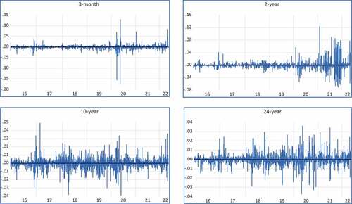
Table 1. Descriptive statistics (across maturities)

	3-month yield	2-year yield	10-year yield	24-year yield
Observations	1593	1593	1593	1593
Mean	0.053291	0.059938	0.068317	0.073624
Median	0.060800	0.063350	0.067540	0.072530
Maximum	0.073500	0.080250	0.081820	0.085820
Minimum	0.027000	0.038610	0.057600	0.063880
SD	0.013949	0.011328	0.006397	0.005019
Skewness	−0.465886	−0.314492	0.192830	0.270117
Kurtosis	1.595105	1.805048	1.820886	2.096414
Jarque-Bera	188.6329	121.0368	102.1540	73.56480
Probability	0.000000	0.000000	0.000000	0.000000
Sum	84.89260	95.48147	108.8286	117.2830
Sum Sq. Dev.	0.309751	0.204304	0.065144	0.040104

Note: Skewness quantifies the asymmetry of the series’ distribution around its mean. A normal distribution has zero skewness. Kurtosis is a measure of the peakedness or flatness of a series’ distribution. The normal distribution has a kurtosis of 3. If the kurtosis is greater than 3, the distribution is leptokurtic, and if it is less than 3, it is platykurtic in comparison to the normal distribution.

In contrast, (O’sullivan & Papavassiliou, 2019) find that volatility increases as maturity buckets increase from shorter to longer. However, their study also revealed that this result is more pronounced during quiet periods. They demonstrate a sharp increase in standard deviation as they move from a calm period into a turbulent one. This indicates that the recent outbreak of the COVID-19 pandemic has pushed uncertainty into the financial market, and this uncertainty has wobbled unprecedented movement in the bond market volatility (Zaremba et al., 2021). Therefore, 3-month treasury and 2-year sovereign bond yields are subject to higher fluctuation levels during the study period since economic activities can directly and immediately impact these rates. In other words, bonds with very long maturities (so-called buy-and-hold bonds) appear to have lower standard deviations because the selling pressure is not as high as bonds with shorter maturities (Friewald et al., 2012). found similar results during the subprime crisis. They found that bonds with shorter maturities were more vulnerable to the crisis than those with longer maturities. The standard deviation values increased from the pre-crisis period to the crisis period, indicating greater volatility. This effect, however, is more apparent during times of crises.

Moreover, the summary statistics show that the non-positively skewed distribution of the yield series is likely to deliver significant negative returns to investors and is more prone to volatility. The high kurtosis ratios show the fatter-tailed distributions of the sovereign bond yield series, which are leptokurtic. In a leptokurtic distribution, outliers are likely to occur, and as a result, distribution tends to be non-normal.

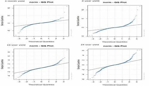
Further, Jarque-Bera test results show t-statistic values of 188.6329 for 3-month treasury yield, 121.0368 for 2-year bond yield, 102.1540 for 10-year bond yield, and 73.56480 for 24-year bond yield with a significant p-value, allowing us to reject the null hypothesis, i.e., distribution follows a normal distribution. As a further instrument to analyze the distributional properties, we use Quantile-Quantile (QQ) graph to check if bond yield series data differ from normality. The QQ plot is a scatter plot that shows the empirical and theoretical quantiles for a given distribution (Alexander, 2001). The results of the QQ plot presented in Figure 2 show the deviation of residuals from the normality line. The greater the deviation from the line, the greater the chance to reject the null hypothesis of the normality assumption. Thus, the graphical representation confirms the findings of the Jarque-Bera test, i.e., Indian Sovereign bond yield data are not normal. These findings support the decision to use an alternate distribution, such as students-t and GED-based GARCH models.

Figure 2. QQ plots of the EGARCH residuals.

This article further contributes to the body of knowledge by examining selected macro-related forces driving the volatility of bond yields. Therefore, Table 2 presents the key descriptive statistics for inflation and Money market volatility in the study at the quarterly frequency. The mean inflation rate reported for the sample period is 4.7514%, with a standard deviation of 1.1598%, implying moderate volatility. Further, the money market rate proxied by the 3-month LIBOR shows an average rate of 1.3616% with a standard deviation of 0.9806%. The descriptive statistics also show evidence for the data normality. It is important to note that a prerequisite for performing the Granger Causality test is that the data need to be normal.

Table 2. Descriptive statistics (macro-economic indicators and sovereign yields at quarterly frequency)

	Inflation (CPI)	Interest Rates (LIBOR)	3-month yield	2-year yield	10-year yield	24-year yield
Observations (Quarterly)	28	28	28	28	28	28
Mean	0.47514	0.13616	0.52226	0.59472	0.67892	0.72961
Median	0.49482	0.12041	0.59050	0.63740	0.66840	0.72190
Maximum	0.66234	0.35652	0.70800	0.78670	0.78530	0.82460
Minimum	0.33282	0.01301	0.30700	0.38650	0.58370	0.64470
SD	0.11598	0.09806	0.13917	0.11229	0.06302	0.04933
Skewness	0.3076	0.3658	−0.3838	−0.2851	0.1533	0.2006
Kurtosis	1.9727	2.0797	1.5446	1.9130	1.8273	2.2395
Jarque-Bera	0.4181	1.5549	2.9329	1.6323	1.5303	0.7701
Probability	0.8113	0.4595	0.2307	0.4421	0.4652	0.6804
Sum	33.2595	36.7637	135.79	154.628	169.7300	182.4030
Sum Sq. Dev.	8.0716	25.0025	48.4257	31.5226	9.5340	5.8417

Note: Skewness quantifies the asymmetry of the series’ distribution around its mean. A normal distribution has zero skewness. Kurtosis is a measure of the peakedness or flatness of a series’ distribution. The normal distribution has a kurtosis of 3. If the kurtosis is greater than 3, the distribution is leptokurtic, and if it is less than 3, it is platykurtic in comparison to the normal distribution.

Furthermore, the descriptive statistics for yields across maturities at a quarterly frequency are presented in Table 2, indicating that the mean and standard deviation exhibit little variation from those reported for daily data; nevertheless, it should be highlighted that while the daily series show non-normal characteristics, the quarterly yield data conform to a normal distribution. Consequently, the linkage between the above macroeconomic determinants and sovereign yield across the maturity spectrum is examined in the study.

Table 3 displays unit root tests performed for each series of Indian sovereign bonds. The Augmented-Dickey Fuller (ADF) and Phillips-Perron (PP) tests were used at a 5% level to examine the stationarity of sovereign bonds of different maturities used in the study. The results of unit root tests show that the calculated values of ADF and PP test statistics are less than the critical value at 5%, implying that all the series are stationarity. Further, the results of the unit root in Table 4 suggest that our data do not meet the stationarity requirements for Granger causality testing. Therefore, original data are transformed using the first differences prior to testing. The results conform to prior expectations, and the coefficients are significant at a 5% level of significance, indicating stationarity for the GDP and 3-month LIBOR series.³

Table 3. Unit root test results

	3-month yield		2-year yield		10-year yield		24-year yield
Test	ADF test	PP test	ADF test	PP test	ADF test	PP test	ADF test	PP test
t-Statistic	−43.348	−43.188	−15.569	−50.529	−40.966	−41.021	−43.877	−43.814
Probability Value	0.0001	0.0001	0.0000	0.0001	0.0000	0.0000	0.0001	0.0001

Note: H0: Sovereign bond yield has unit root one (non-Stationary)

Table 4. Unit root test results for macroeconomic variables

	Inflation (CPI)		Interest (LIBOR)
Test	ADF test	PP test	ADF test	PP test
t-Statistic	−3.6948	−3.6948	−2.9981	−1.0511
Probability Value	0.0018	0.0055	0.0376	0.0197

Note: H0: Sovereign bond yield has unit root one (non-Stationary)

Following the unit root test, we applied the Lagrange multiplier (LM) test to check for the presence of the ARCH effect in our data set. The reported results in Table 5 show the prevalence of the ARCH effect in all yield series. Thus, to assess the conditional volatilities of the Indian sovereign bond yield over four distinct maturities, GARCH family models (standard GARCH, IGARCH, EGARCH, and GJR-GARCH) are applied.

Table 5. ARCH LM test results

	3-month yield	2-year yield	10-year yield	24-year yield
ARCH LM test statistic	130.2611	57.18295	10.03185	47.23850
Probability Value	0.0000	0.0000	0.0016	0.0000

Note: H0: There are no ARCH effects in the sovereign bond yield.

5. Empirical analysis and discussion

5.1. Model selection, volatility persistence, and leverage

5.1.1. Preliminary analysis and model selection

As reported, data in Table 5 provides strong evidence against the null hypothesis, i.e., data are homoscedastic; we conclude that the government bond yield series shows heteroscedasticity, or the presence of the ARCH effect is confirmed. Thus, to model this conditional variance, we proceed with the GARCH family models. Further, we estimate models based on the maximum likelihood approach under the assumption of GED (Since AIC and BIC values under GED are lower over the student’s t distribution). The GARCH (1,1) model results with GED and Student’s t distribution are reported in the Appendices (2, 3, 4, and 5). The GARCH model shows that the ARCH term and GARCH term are statistically significant across maturities. This implies that the conditional variance of the bond yield series is significantly impacted by the lagged conditional variance and squared disturbances, implying that volatility news of previous time periods impacts the current days’ volatility. Further, the sum of α and β coefficients across four maturities is less than unity, implying the validity of the GARCH (1,1) model. However, symmetric GARCH models cannot differentiate the impact of the “leverage effect” on the conditional variance of bond yield data. Hence, we further proceed by applying popular asymmetric-type GARCH models to measure the impact of positive and negative shocks. The results of asymmetric GARCH models are presented in the Appendix. We have applied the maximum likelihood approach to choose the best model that fits our data set (Maximum likelihood value, refer to Appendix). The EGARCH model is the best model across 3-month, 2-year, 10-year, and 24-year sovereign series.

5.1.2. Empirical analysis on GARCH (1,1), IGARCH and GJR-GARCH

The dynamics of the volatility of sovereign yields and their persistence across maturity buckets are examined using GARCH (1,1), IGARCH, and GJR-GARCH.⁴ The results of the GARCH (1,1) model show that all the coefficients are highly significant (Refer to appendix 2, 3, 4, and 5). The stated α measures how much a volatility shock of the current day affects volatility in the following period (Campbell et al., 1997). The coefficients of the 3-month, 2-year, 10-year, and 24-year sovereign series are 0.084712, 0.104348, 0.119837, and 0.083868, demonstrating the presence of volatility clustering. However, the coefficients for IGARCH and GJR-GARCH show comparable results. For identical maturity periods, the coefficients for IGARCH are 0.06464, 0.105391, 0.120626, and 0.167508, whereas the coefficients for GJR-GARCH are 0.052954, 0.054199, 0.126086, and 0.149875. The coefficient has been significant for the series, demonstrating that historical lags cannot affect future volatility. However, the negative estimate on the “alpha” component indicates that adverse shocks provide lower next-period conditional variance than positive shocks of the same sign (Brooks, 2019).

The β coefficient estimate implies that the variance has a long memory. However, the GARCH term is statistically significant for each maturity spectrum across different GARCH specifications employed in the current study. For 3-month, 2-year, 10-year, and 24-year sovereign series, the estimated GARCH coefficients for GARCH (1,1) are 0.897382, 0.89454, 0.879163, and 0.910881, suggesting that changes in current volatility have a long-term impact on future volatility. Furthermore, the β coefficients for IGARCH and GJR-GARCH are approximately comparable to the GARCH (1,1) and EGARCH results. For 3-month, 2-year, 10-year, and 24-year sovereign series, the IGARCH coefficients are 0.93536, 0.894609, 0.879374, and 0.802731, respectively. Besides, the coefficients for GJR-GARCH for the same maturity frame are 0.890587, 0.911427, 0.880148, and 0.800982, indicating that volatility shocks are quite persistent. Nevertheless, the results support the growing body of literature documenting that shocks are not immediately absorbed.

Moreover, the results of the GJR-GARCH model, an alternative to the EGARCH model, are in accordance with EGARCH results, particularly for the measurement of asymmetric volatility. The reported results show that the leverage coefficient γ (gamma) is significant and positive across all the maturities, implying that the positive shocks create higher volatility than the negative ones.

5.1.3. Volatility persistence and asymmetry based on EGARCH results

Based on the AIC and BIC values (lowest value), the EGARCH model with GED is considered in the study (Refer to Table 6 and 7). However, the Log-Likelihood is maximum under Student’s t for the 10-year bond. It is also important to note that their performance is almost identical due to the negligible difference in the AIC and BIC values between GED and Student’s t. Moreover, the EGARCH is often the superior model for predicting volatility in a single phase.

Table 6. EGARCH results

Parameter	Distribution Type	3-month yield	2-year yield	10-year yield	24-year yield
µ (MU)	Normal	−0.000405***	0.000091	−0.000029	0.000080
	Student’s t	−0.000271***	−0.00032***	−0.000052	0.000154
	GED	0.000000	−0.000100***	0.000000	0.00000
Ω (Omega)	Normal	−0.089692***	−0.003373***	−0.112156***	−0.253970***
	Student’s t	−0.627056***	−0.11541***	−0.247236***	−0.453559***
	GED	−0.97271***	−0.110040***	−0.231378***	−0.49158***
α (Alpha)	Normal	−0.076940***	0.035663***	0.002634	0.003083
	Student’s t	−0.136383***	−0.20987	0.001048	−0.028684
	GED	−0.26038***	−0.016005	0.003112	−0.01833
β (Beta)	Normal	0.985170***	0.996215***	0.987394***	0.972437***
	Student’s t	0.932585***	0.98154***	0.975297***	0.928131***
	GED	0.90361***	0.988233***	0.977324***	0.948029***
γ (Gama)	Normal	0.314314***	0.151169***	0.138774***	0.212423***
	Student’s t	0.522368***	1.13358***	0.255290***	0.621886
	GED	0.81360***	0.257037***	0.210311***	0.30120***

Notes 1: *, **, ***: Statistically significant at the 10%, 5%, and 1% level of significance, respectively.

2: In the EGARCH results, the term ‘Omega’ represents the constant part: a kind of ‘Ambient Volatility’, Alpha represents the adjustment to past shocks, the Beta term represents an adjustment to past volatility and long-run memory of the current volatility pattern, Gama represents ‘leverage coefficient’ or the influence of good and bad news on the current volatility.

Table 7. Distribution selection under EGARCH

	Distribution Type	3-month yield	2-year yield	10-year yield	24-year yield
AIC (Akaike)	Normal	−7.0532	−6.7158	−7.3634	−7.5603
	Student’s t	−7.4912	−7.2615	−7.5876	−7.8800
	GED	−8.1640	−7.2935	−7.5749	−7.9078
BIC (Bayes)	Normal	−7.0362	−6.6988	−7.3465	−7.5434
	Student’s t	−7.4675	−7.2378	−7.5639	−7.8563
	GED	−8.1437	−7.2732	−7.5546	−7.8875
Log-Likelihood	Normal	5594.626	5327.234	5840.498	5996.537
	Student’s t	5943.768	5761.774	6020.156	6251.921
	GED	6476.008	5786.079	6009.13	6272.946

Note: Student’s t and GED are non-normal distributions. The AIC and BIC values determine the best distribution for the data set. Distribution with the lowest AIC/BIC value can be regarded as the best suitable distribution. Similarly, the log-likelihood determines the best asymmetric GARCH models for the data set considered in the study, and we have followed the maximum likelihood approach. Thus, the EGACRH model with GED turns out to be the best model for our data set (Refer to appendix for the results of other models).

The EGARCH model results are shown in Table 6 for the yields series on 3-month, 2-year, 10-year, and 24-year treasury securities (Columns 3, 4, 5, and 6). The adoption of the asymmetric volatility model is supported by the fact that the leverage coefficient γ for each type of government security is statistically significant at the 1% level. In the model, the stated α measures how much a volatility shock today affects volatility in the following period (Campbell et al., 1997). The α coefficients for our series of sovereign yields, which include 3-month, 2-year, 10-year, and 24-year, are −0.26038, −0.016005, 0.003112, and −0.01833, respectively. The coefficient is statistically significant for the 3-month benchmark yield while insignificant for other sovereign bond yields across maturities, demonstrating that historical lags can affect future volatility only in the near term. However, the negative estimate on the “alpha” component indicates that negative shocks provide lower next-period conditional variance than positive shocks of the same size (Brooks, 2019).

The estimation of the β coefficient indicates a long memory in the variance. The correlation structure of a specific series at long lags is referred to as having a “long memory.” Distance observations have persistent temporal dependency if a series demonstrates long memory. The potential for long-term dependence on sovereign yield significantly impacts the financial time series. The long-memory quality of financial time series has been studied in the existing literature. Security returns, for instance, exhibit a positive correlation over short time horizons and a negative correlation over long time horizons, according to Poterba (Poterba & Summers, 1988). As the holding period increases, the negative serial correlation between sovereign yields becomes more pronounced. This result is implied by the mean-reverting model’s long-term memory property. According to (Lo 1991) long-horizon yields may be characterized by long cycles and potentially predictable components.

The GARCH term (β) is statistically significant for sovereign yield series across maturity buckets considered in the study. The estimated coefficients are 0.90361, 0.988233, 0.975297, and 0.948029 for the 3-month, 2-year, 10-year, and 24-year series, respectively. Further, the coefficients are close to unity, implying that changes in the current volatility will have a long-term impact on the future volatility or that the impact of previous news on the current volatility is long-lasting. Besides, a high long-memory coefficient shows that the asset exhibits a long positive or negative stray from equilibrium. As a result of its inability to effectively protect investors from volatile market conditions, such security is no longer considered a good hedge or safe haven.

Moreover, long memory qualities and asymmetric impacts are stylized facts likely to result in significant financial outcomes. A time series is regarded as having long memory and asymmetric behaviour when its corresponding autocorrelation function is non-integrable. In reality, the fundamental result of long memory is its nonlinear dependence during the first and second moments (Elder & Serletis, 2008). The results, however, confirm that shocks to sovereign yields may take longer to dissipate, but they are not permanent. If a shock to a given system is lasting, volatility is highly persistent, and the behaviour of volatility in the past can be utilized to forecast future volatility. However, normal times with relatively stable pricing may be followed by periods with significant volatility. Because information decays slowly in such markets, old information is more important than new knowledge. This is evidence of so-called long memory behaviour. In view of the financial implications of these coefficients, investors can construct future positions in anticipation of this feature. In contrast, low volatility persistence suggests that the shock response function could decay quickly. Low persistence equates to rapid decay and quick reversion to the mean.

5.1.4. EGARCH asymmetry, leverage, and shocks

The result for the EGARCH asymmetry term (γ) shows a positive coefficient for different maturities considered in the study. According to the EGARCH results reported in Table 6, positive shocks/news cause more volatility in the subsequent period than negative return shocks or news of the same size. For each bond across all maturities, γ is positive and statistically significant at the 0.01 level. Further, γ the leverage coefficient is as high as 0.81360 for the 3-month treasury, 0.257037 for the 2-year bond, 0.210311 for the 10-year bond, and 0.30120 for the 24-year bond.

The leverage effect refers to the well-established negative relationship between return and future volatility. The relation is usually explained by the increased leverage ratio that arises from a drop in the share price for a firm. As the price of a stock falls, its debt-to-equity ratio rises, increasing the volatility of returns to equity holders (Black & Cox, 1976). A stylized characteristic of financial volatility is that negative shocks (bad news) influence volatility more than positive shocks (good news), where the focus is on equity returns (Aliyev et al., 2020b; Bhatia & Gupta, 2020; Wang et al., 2022).

However, in this paper, we concentrate on sovereign bond yields. This contradicts the assumption of the Black and Scholes model, where the focus is on the corporate debt-to-equity ratio (Black & Cox, 1976; Black & Scholes, 1973). This article defines leverage as the ratio of sovereign debt-to-GDP (Bauer & Granziera, 2016; Pintus & Suda, 2013; Sun, 2018). In the context of sovereign bonds, a decrease in yield increases the expected future volatility. A lower yield is often perceived as an indicator of higher risk and lower income. However, a low yield may have resulted from a rising market value of the sovereign bond, which increases the total sovereign debt and leads to the leverage effect (i.e., a higher sovereign debt-to-GDP ratio). Therefore, a positive shock leads to increasing sovereign bond prices and induces, by statistical definition, a lower yield.

According to (Cecchetti and Zampolli 2011) low and moderate levels of debt help promote welfare and economic growth, whereas high levels can be a disaster. The study suggests that a lower debt-to-GDP ratio can reduce the likelihood of a financial crisis, indicating a threshold effect of debt. When the debt level exceeds the threshold value, it has negative impacts on GDP and raises leverage, ultimately leading to a more disturbed economy. While the attention of policymakers following the recent crisis has been on reducing systemic risk stemming from a highly leveraged financial system, the system demands less leveraged and ultimately less risky economies.

Our findings are the exact opposite of what one would expect when applying a GARCH model to a set of stock returns. The impact of positive shocks is recognized in the extant research as the “anti-leverage” effect, as theoretically documented by (Nelson, 1991) and (Glosten, Jagannathan, & Runkle, 1993). Over time, various studies have shown the significance of such an effect on the relationship between corporate bonds and equity (Ghysels et al., 2005; Harrison & Zhang, 1999; Ludvigson & Ng, 2007). However, this paper uses yields rather than returns, and a price rise is associated with a yield fall (Fabozzi, 2021), which leads to “regular leverage”. In summary, our findings suggest that a positive policy shock elicits greater volatility in sovereign yields relative to negative shocks of equivalent magnitude.

According to our findings in this section, the amount of persistence differs across the type of sovereign yield series, with medium-term and long-term possessing more persistence than short-term series. Besides, the type of GARCH model employed is a critical choice in modelling conditional volatility. The EGARCH model with GED (3-month, 2-year, and 24-year) and Student’s t (10-year) was found to be the best-fit model to the yield data as it exhibits lower forecast errors and provides a better description for the conditional volatility. Overall, investors should be aware that the volatility of the Indian sovereign yield is more sensitive to good news across the maturity spectrum to cover potential losses. However, it is important to examine the properties of the yield in both bull and bear periods to better understand how it behaves in different market conditions. Therefore, we examine the properties in the bull and bear periods, testing if the degree of persistence is different in these periods in our series in the next section.

5.2. Volatility persistence and mean-reversion: Comparison between bull and bear markets

This section deals with the analysis of volatility persistence in the bull and bear phases of the Indian sovereign yield series across different maturity specifications. Since the COVID-19 pandemic, the globe has recently seen one of its worst bear markets, making it especially important to academic research. We assume that there are bull and bear market phases and that each market phase is a regime that is influenced by particular market forces. These market forces produce negative news, which causes panic and prompts investors to sell off bonds quickly. When there is no more bad news, markets bounce back. However, investors retain bonds during bull markets when a string of good news generates optimism, while they sell bonds during bear markets due to pessimism.

This sample period selected for the study saw a significant surge and a sharp decline in the market as COVID-19 unfolded. It provides a perfect context to investigate whether the relationship differs in bull and bear markets. We divide the sample period into bull and bear phases using the methods proposed by (Conlon et al. 2021) and (Conlon & McGee, 2020). Accordingly, the bull market lasted from 1st April 2016 to 10th March 2020, while the bear market lasted from 11 March 2020 to 18 May 2022. This isolates the impact of the COVID-19 pandemic and captures the bear market.⁵ In line with (Rahman and Lee 2002) our findings show that the EGARCH (1,1) model best captures volatility with GED distribution over maturities for both phases.

For the purpose of modelling financial time series, the study of persistence and half-life is pivotal. They aid in figuring out how long it takes to return to the mean and whether the estimated GARCH model is stable. A model that gauges the average time (also known as the mean reversion speed) of the yields under investigation is the half-life volatility of the EGARCH model. Therefore, we quantify the days in which yields revert to the mean in accordance with (Bhar and Nikolova 2009), Fakhfekh et al. 2016) and (Jane & Ding, 2009). The volatility of the half-life can be expressed as

$Half-life=\frac{ln\left(0.5\right)}{ln\left(\beta \right)}$

However, the sovereign yield series shows evidence of long-memory behaviour during the bull market, as reported in Table 5. The results show that volatility persistence in bull phases is longer in general throughout the reference period. Gains during market expansions outnumber losses during market cycles’ bear phases. This study shows that when news enters the market during a bullish period, investors in Indian government bonds do not react to new information until a market trend is well established. As a result, a large amount of information is gathered and unexpectedly established in the market, causing volatility in sovereign yields across maturities.

Table 8. EGARCH results during pre-COVID-19

Parameter	Distribution Type	3-month yield	2-year yield	10-year yield	24-year yield
α (Alpha)	GED	−0.02656 ***	−0.029940	−0.018020	−0.060160
β (Beta)	GED	0.864455 ***	0.968846***	0.984466***	0.976944***
Ln(0.5)		−0.69315	−0.69315	−0.69315	−0.69315
Ln(β)		−0.14566	−0.03165	−0.01566	−0.02333
Mean Reversion in days		4.7588	21.9006	44.2738	29.7157

Note: *, **, ***: Statistically significant at the 10%, 5%, and 1% level of significance, respectively.

The findings of our half-life approach calculation of mean reversion speed are reported in Table 8. The findings show that the 10-year government bond yield has the highest $\beta$ coefficient (0.984466); as a result, it takes the longest period (44.2738 days) to return to half of its mean among all maturities during a bull market. The 3-month Treasury yield, in comparison, has the lowest value of 0.864455 because it takes the least amount of time (4.7588 days) to return to half of its mean when compared to other maturities during a bullish phase. However, the yields on sovereign bonds with a 2-year and 24-year maturity return to half of their mean in 21.9006 and 29.7157 days, respectively.

This suggests that investors in 10-year sovereign bonds must initiate a position at 0 days and close after 88.5476 days because the yield on 10-year sovereign bonds shows that the yields returned to half their mean value within 44.2738 days. The slowest mean reversion process occurs in the 3-month treasury yield; therefore, investors should start at 0 days and close after 9.5176 days. Thus, compared to the 3-month treasury yield, which offers the least time period for investors to act freely, the 10-year sovereign bond gives them maximum operating leverage.

Based on the results (Table 9) for the EGARCH parameters and the trajectory of COVID-19, we discover that yield volatility is more persistent in bull market than in bear market except in 3-month series. Recent literature is consistent with the size of the volatility persistence as shown by $\beta$ for the Indian sovereign bond market (see (Koulakiotis & Molyneux, 2006). Intriguingly, during times of stress (a bear market), certain yield series across different maturities, such as the 3-month Treasury yield, 2-year Sovereign Bond yield, 10-Year Sovereign Bond yield, and 24-Year Sovereign Bond yield, tend to have lower levels of volatility persistence (0.914978, 0.951023, 0.965075, and 0.655224, respectively), indicating that they are better able to withstand the shocks to which they are exposed (see (Taing & Worthington, 2005; Young & Johnson, 2004).

Table 9. EGARCH results during the COVID-19 era

Parameter	Distribution Type	3-month yield	2-year yield	10-year yield	24-year yield
α (Alpha)	GED	−0.23636***	−0.308765	−0.354528	0.005480
β (Beta)	GED	0.914978***	0.951023***	0.965075***	0.655224***
Ln(0.5)		−0.69315	−0.69315	−0.69315	−0.69315
Ln(β)		−0.08886	−0.05022	−0.03555	−0.42278
Mean Reversion in days		7.8008	13.8030	19.4981	1.6395

Note: *, **, ***: Statistically significant at the 10%, 5%, and 1% level of significance, respectively.

The findings further (Table 9) indicate that the mean-reversion process has been proven to exist for each of the four sovereign yield maturities. In contrast to the bullish phase, which exhibits a faster mean reversion rate across similar maturities, the yields on Indian sovereign bonds across maturities indicate moderate volatility and sluggish mean reversion. The 10-year sovereign bond has the lowest mean reversion in days, whereas the 3-month treasury yield has the highest mean reversion in days. The 3-month Treasury yield returns to its mean position in 15.6016 days, according to the half-life calculation, while the 2-year Sovereign Bond Yield does so in 27.606 days. In 38.9962 days, the 10-year sovereign bond yield returns to its mean level, whereas the 24-year sovereign bond yield comes back to its mean value in 3.279 days. Our results are consistent with those of (Ledwani et al., 2021), who show that the detrimental effects of COVID-19 had diminished more quickly in the Indian financial markets, supporting the market correction following the panic-induced decline. The market overreaction theory and market correction theory explain the markets’ collapse and quick rebound. The government’s implementation of strong control measures has effectively curtailed the spread of COVID-19 and decreased the volatility of sovereign yields across the maturity buckets. The various fiscal support policies implemented by governments around the world have also played a positive role in curbing sovereign yield fluctuations. Based on the results of the empirical and theoretical analyses in this article, government interventions can effectively reduce the uncertainty and panic caused by COVID-19, and send positive signals to the markets and investors, resulting in faster mean reversion. However, a low level of government intervention and lack of access to other markets contribute to the high volatility and slow mean reversion in emerging economies. The findings are in line with those of (Al-Hajieh, 2017; Chaves & Viswanathan, 2016; Sharma et al., 2021). Through the above contributions, we offer concrete recommendations for the implementation of government policies in the future.

According to Iyiegbuniwe et al., (2012), market booms in developing markets cause greater volatility than market declines, which is justified by the idea that investors think booms act more like speculative bubbles. In contrast to the findings (Nelson 1991) claims that volatility is higher in bearish phases because investors are more likely to engage in panic selling during these times. According to the findings, the Indian sovereign bond yields experienced volatility during the pandemic era. However, when comparing the COVID-19 period to the pre-COVID period, we discovered that mean reversion is slower in the pre-COVID-19 period than during the COVID-19 period. In this regard, the outcomes of bull and bear market cycles are states with persistent and statistically significant variations in mean returns.

As we confirm from our well-established volatility analysis, the speed of mean reversion varies with the market phase under study. We find that volatility generally responds more markedly to shocks during the period under stress (a bear market). In contrast, sovereign yield volatility during the bullish phase is highly persistent; when it rises, it remains high for a considerable time and returns to its mean only gradually. These findings suggest that the Indian sovereign bond yield is influenced by a range of economic factors and that its behaviour may change over time. Therefore, we seek to empirically analyse the linkage between the sovereign bond yield volatility and selected macroeconomic determinants in India across maturity spectrum in the next section.

5.3. Macro-related forces and sovereign yield volatility

In this section, we take a first step towards answering a research question of the paper: how do macroeconomic shocks affect sovereign yield volatility across the maturity spectrum? The Granger causality test is widely used in research to identify such a relationship, as stated by (Bui, 2018). We test here for Granger causality between interest rate volatility (3-month LIBOR), as well as the inflation, on the one hand, and the sovereign yield volatility (computed either using a 3-month or a 2-year or a 10-year or a 24-year window), on the other hand.⁶ The role of this step is to establish, in a bivariate setting, whether the selected macroeconomic variables have predictive power with respect to the sovereign yield volatility across the maturity spectrum and vice-versa.⁷

The results for Granger causality are shown in Tables 10 and 11. The non-existence of unit roots justifies the approach as reported in Table 3 for macroeconomic determinants and Appendix 1 for quarterly yield series. This is a common approach to determine whether a particular series is stationary, whether a trend characterizes it, or takes the shape of a stochastic trend or a deterministic or linear trend. The Granger causality test would produce inaccurate results if there were a unit root, which suggests non-stationarity.

Table 10. Granger casualty test for the linkage between sovereign bond yield volatility and inflation

	3-month yield	2-year yield	10-year yield	24-year yield
	F-Statistic	F-Statistic	F-Statistic	F-Statistic
Inflation does not Granger cause Bond yield volatility	4.19187**	5.35855**	4.61866**	3.62401**
Bond yield volatility does not Granger cause Inflation	2.30873	1.11131	2.71625	1.04665

Note: *, **, ***: Statistically significant at the 10%, 5%, and 1% level of significance, respectively.

Table 11. Granger casualty test for the linkage between sovereign bond yield volatility and money market volatility

	3-month yield	2-year yield	10-year yield	24-year yield
	F-Statistic	F-Statistic	F-Statistic	F-Statistic
Money Market Volatility does not Granger cause Bond yield volatility	3.12562***	3.385210**	3.98426**	3.36984**
Bond yield volatility does not Granger cause Money Market Volatility	4.32622***	3.64875**	3.78358**	3.81264**

Note: *, **, ***: Statistically significant at the 10%, 5%, and 1% level of significance, respectively.

5.3.1. Sovereign bond yield volatility and inflation

Over time, the link between movements in bond yields and fundamental economic forces, such as expectations about inflation, is not as well established as over the long-term or across countries at a point in time. For instance, debate continues about whether the change in the level of yields over the last couple of years is explicable in terms of such fundamentals. In general, the shorter the time horizon, the more likely it is that market participants generate yield movements themselves. The close association between the long-term inflation record and the level of bond yields across countries supports this relationship. At the same time, there is considerable evidence that bond yields play an important role in setting the background level of volatility, pointing to a role for inflation.

The findings of testing for Granger causality are shown in Table 10. The findings suggest that Granger causality exists for inflation. Across the maturity spectrum, the evidence is robust. In contrast, there is no evidence of Granger causality from sovereign yield volatility to inflation. In these cases, the link is probably disturbed by the sharp but short-lived movements in short-term rates in response to strains in the other macroeconomic determinants.

Our findings align with (Wesso, 1998) and (Zhou 2021) who investigate the relationship between expected inflation and yield behaviour. According to the analysis, inflationary pressures are not predicted by sovereign yield. However, it has been found that inflation positively and considerably impacts sovereign yields in India. However (Ntshakala and Harris 2018) contend that the slope of the yield curve affects expected inflation, rejecting the idea that the term structure determines the direction of inflation.

The findings show that long-term and short-term bond yield volatility is increased by an economy’s inflation history and expectations and that changes in inflation are likely to have the strongest impact on bond yields. Additionally, the inflation rate has an impact on government bond yields because investors consider it as a proxy for uncertainty and instability, which raises risk premiums and, as a result, the level of yields (Baldacci & Kumar, 2010; Baldacci et al., 2008; Cantor & Packer, 1996).

5.3.2. Sovereign bond yield volatility and money market volatility

We next examine the link between money-market volatility and bond yield volatility. Just as one can ask what happens to the bond rate when short-term rates change, so one can trace the movements of the volatility of the bond rate associated with changes in money-market volatility. Volatile money markets create more volatile bond markets. In theory, such money market volatility can be linked to the modus operandi; of monetary policy, but the precise nature of the link remains an important research subject. The precise interpretation of the link between the money market and bond yield volatility will partly depend on the measure of volatility used. In keeping with our emphasis on uncertainty, we employed a forward-looking indicator, a 3-month LIBOR (Bandholz et al., 2009). In fact, this rate can be taken as an admittedly rough approximation to market expectations of the money market volatility.

We examine the relationship between sovereign yield volatility and money market volatility in the Indian credit market for government bonds. The test results reported in Table 11 show that there is Granger causation between sovereign yield volatility and money market volatility in general. However, for each series, we found a bidirectional link between these two factors.

Keynes’s claim is supported by a number of recent empirical studies on the dynamics of government bond yields, which show that after adjusting for relevant macroeconomic and financial variables, there is a substantial correlation between interest rates and sovereign yields. These findings are relevant to macroeconomic theory and policy (Akram, 2021). These findings support the conclusions of (Akram & Das, 2015a, 2015b, 2019), who state that interest rates play a leading role in driving fluctuations in sovereign bond yields in India. The conclusions are consistent with those obtained in research by (Chakraborty (2012) and (Vinod and Chakraborty 2014) despite the fact that the econometric and statistical approaches used are somewhat different. This finding has significant policy concerns. It suggests, for instance, that decisions about money market rates affect yields over the medium- and long-term, in addition to their direct impact on short-term yields. As a result, the key finding that the interest rate is the main factor influencing sovereign bond yields remains true regardless of the maturity parameters.

The results reported in Table 11 also generate predictions about the strength of granger casualty from sovereign yield volatility to money market volatility. In particular, our results reveal strong causation from 3-month sovereign yield volatility to money market volatility. The intuition behind the strong linkage between sovereign yield volatility and money market volatility is straightforward. An information event that alters the sovereign yield volatility directly affects the money market volatility measured using 3-month LIBOR. Since both sovereign yield volatility and money market volatility are strongly correlated, it might seem reasonable to attribute the linkages solely to common information. Stronger linkages occur with higher levels of common information and information spillover. The common information flow should be high between markets with security values driven by similar underlying fundamentals (Fleming et al., 1998). However, the results based on time-series estimates of the information suggest that the relationship becomes weaker as the sovereign yield maturity increases.

Our paper concludes that the Indian sovereign yields cannot be dissociated from inflation and money market volatility. Since, in the long-term, inflation performance and expectations are probably the main influence on yields, a similar claim can be made for money market volatility to the extent that it, too, contributes to the volatility of yields. Money market volatility can cause bond yield volatility, and our results show that the reverse is also possible. Each market is influenced by macroeconomic information, and the characteristics of these markets are conducive to cross-market hedging. Therefore, we expect to observe strong volatility linkages. Hence, the link between such fundamental economic factors and their movements cannot be taken for granted. In summary, given the strong linkage between sovereign yield volatility and money market volatility, the common determinants affecting these variables need to be determined in future research. However, it is also worth noting that there may be other macroeconomic determinants that could also have an impact on the Indian sovereign yields, such as GDP growth, exchange rates, and fiscal policy. It is important to consider these other factors as well, as they can provide a complete picture of the market dynamics.

6. Conclusions

In this paper, we model and estimate the volatility of sovereign bond yields across short, medium, and long-term maturities. The findings demonstrate that the yield series on sovereign bonds deviates from normality and exhibits volatility clustering with varying residual variance. Further, the conditional variance of the returns exhibits a nonlinear structure which necessitates the need to use the appropriate models for effectively estimating volatility in the Indian government bond yields. In order to account for the long-memory and asymmetric effects, our research has focused on the GARCH-family models. The EGARCH with GED is the best model fit for the 3-month, 2-year, and 24-year sovereign yield volatility series after applying four GARCH specifications with different related error distributions, including the GARCH (1,1), EGARCH, IGARCH, and GJR-GARCH models. On the other hand, with the 10-year bond, the Log-Likelihood is at its highest under Student’s t distribution, which can be ignored as there is a negligible difference in AIC and BIC values. However, the EGARCH model is frequently the best model for making predictions within a single phase.

The mean-reverting process is supported by the estimates of the model parameter β, which demonstrate that the series variance has a long memory and that volatility shocks are highly persistent for medium and long-term series but non-unity. The short-term series decays faster compared to the strong volatility persistence of the medium and long-term maturity. Furthermore, it has been found that volatility tends to rise in reaction to positive shocks as opposed to negative shocks of equal magnitude, suggesting the possibility of a “leverage effect” that is markedly different from that frequently seen in stock markets.

Besides, results indicate that, as inflation and expectations are the primary influence on yields, bond yield volatility rises as revisions in market expectations about inflation take place. Further, money market volatility causes bond yield volatility and vice-versa. We relate this finding to the presence of heightened market discipline within the Indian credit market and money market. Building on the well-developed analysis of volatility, we confirm that when bond volatility rises, it returns to its mean quickly during the period under stress (a bear market) except for the 3-month sovereign yield. As opposed to that, during bullish periods, Indian sovereign bond yields are highly persistent; when they rise, they remain high for a long period and then return to their mean only gradually.

Our research also explores the relationships among COVID-19, government intervention, and sovereign yield volatility during the bearish phase. For government responses, our research supports faster mean reversion during the bearish phase. When a government adopts various intervention policies for COVID-19, it should fully consider the resultant impacts and make an effort to eliminate any adverse ones on the overall economy.

Disclosure statement

No potential conflict of interest was reported by the authors.

Additional information

Funding

The authors received no direct funding for this research.

Notes on contributors

Lithin B M

Lithin B M (First Author) is a Doctoral Scholar. His area of research is corporate finance and is currently pursuing his Ph.D. from theManipal Academy of Higher Education, Manipal, India

Suman Chakraborty

Suman Chakraborty (Corresponding Author) is working as an Associate Professor at the Department of Commerce, Manipal Academy of Higher Education, India. His research areas are Corporate Finance, Financial Markets, and Business Valuation.

Vishwanathan Iyer

Vishwanathan Iyer is a senior Associate Professor in the area of Accounting and Finance and currently the Dean (Accreditation) at the Great Lakes Institute of Management. His research interests are Portfolio Optimization, Earnings Management, Information content of text-based narrative in Annual reports, and the role of inspirational potency in communication to stock market participants.

Nikhil M N

Nikhil M N is currently pursuing his Ph.D. from the Department of Commerce, Manipal Academy of Education, Karnataka, India. Nikhil’s research is on capital structure and firm performance.

Sanket Ledwani

Lithin B M (First Author) is a Doctoral Scholar. His area of research is corporate finance and is currently pursuing his Ph.D. from theManipal Academy of Higher Education, Manipal, India

Sanket Ledwani is currently pursuing his Ph.D. from the Department of Commerce, Manipal Academy of Education, Karnataka, India. Sanket’s research is on Equity Level expected returns and Earnings Predictability.

Notes

1. In fact, this was an explicit policy of rating agencies until 1997. Although this relationship persisted after 1997, empirically document it. In a recent paper, examine the influence of sovereign risk on corporate risk in emerging markets with option-adjusted spreads. More recently, examined the characteristics of bonds rated higher than their sovereigns.

2. There is a reason why sovereign credit risk spills over to corporate credit risk, which is called the “transfer risk”: By increasing corporate taxes, imposing foreign exchange controls, and even expropriating private investment, a government in financial distress will likely shift the debt burden onto corporations.

3. Stationarity results for Sovereign yields quarterly series are reported in Appendix 1.

4. The results of GARCH (1,1), IGARCH and GJR-GARCH are reported in Appendx 2, 3, 4, and 5.

5. A bear market is colloquially regarded as one where the stock market decreases by more than 20%. In the case of the COVID-19 crisis this initial decline occurred between 13th February and 12th March 2020.

6. To measure the volatility for sovereign yields and 3-month LIBOR, we follow (O’sullivan & Papavassiliou, 2019) and measure volatility by the standard deviation for each series.

7. The number of lags used in Granger Casualty test for each series is 2.

Appendices Appendix 1.

Unit Root Test Results for Sovereign Yield at Quarterly Frequency

Table

	3-month yield		2-year yield		10-year yield		24-year yield
Test	ADF test	PP test	ADF test	PP test	ADF test	PP test	ADF test	PP test
t-Statistic	−2.9918	−2.9918	−2.9918	−2.9918	−2.9980	−2.9980	−2.9980	−2.9980
Probability Value	0.0067	0.0097	0.0326	0.0370	0.0022	0.0021	0.0003	0.0003

Note: H0: Sovereign bond yield has unit root one (non-Stationary)

Appendix 2a. 3-Month Treasury Yield

Table

		GARCH (1,1)	GJR-GARCH	IGARCH
µ	Normal	−0.000125	−0.000179	−0.000125
	Student’s t	−0.000140	−0.000186	−0.000140
	GED	0.000000	0.000000	0.000000
Ω	Normal	0.000001	0.000001	0.000001
	Student’s t	0.000005***	0.000005***	0.000005***
	GED	0.000000	0.000000	0.000000
α	Normal	−0.124864***	0.091242***	0.124582***
	Student’s t	−0.286370***	0.161999***	0.286682***
	GED	−0.084712***	0.052954***	0.06464***
β	Normal	0.874136***	0.872288***	0.875418
	Student’s t	0.712630***	0.710942***	0.713318***
	GED	0.897382***	0.890587***	0.93536***
γ	Normal		0.070938***
	Student’s t		0.260461***
	GED		0.081369***

Note: *, **, ***: Statistically significant at the 10%, 5%, and 1% level of significance, respectively.

Appendix 2b. Distribution Selection for 3-Month

Table

		GARCH (1,1)	GJR-GARCH	IGARCH
AIC	Normal	−7.0177	−7.0271	−7.0199
	Student’s t	−7.4705	−7.4779	−7.4718
	GED	−7.9678	−7.9469	−8.0218
BIC	Normal	−7.0042	−7.0101	−7.0097
	Student’s t	−7.4502	−7.4542	−7.4549
	GED	−7.9508	−7.9266	−8.0082
LogLikelihood	Normal	5565.549	5573.946	5566.261
	Student’s t	5926.387	5933.226	5926.433
	GED	6319.45	6303.9	6361.248

Appendix 3a. 2-Year Sovereign Bond Yield

Table

		GARCH (1,1)	GJR-GARCH	IGARCH
µ	Normal	−0.000142	−0.000144	−0.000145
	Student’s t	−0.000258***	−0.000259	−0.000145***
	GED	−0.000100***	−0.000200***	−0.000100***
Ω	Normal	0.000000	0.000000	0.000000
	Student’s t	0.000002	0.000001	0.000002
	GED	0.000001	0.000000	0.000001
α	Normal	−0.052424***	0.072798***	0.052936***
	Student’s t	−0.184439***	0.119272***	0.182315
	GED	−0.104348***	0.054199***	0.105391***
β	Normal	0.946576***	0.945179***	0.947064
	Student’s t	0.814561***	0.835069***	0.817685
	GED	0.894544***	0.911427***	0.894609***
γ	Normal		−0.037954***
	Student’s t		0.087720***
	GED		0.025154

Note: *, **, ***: Statistically significant at the 10%, 5%, and 1% level of significance, respectively.

Appendix 3b. Distribution Selection for 2-Year

Table

		GARCH (1,1)	GJR-GARCH	IGARCH
AIC	Normal	−6.7251	−6.7355	−6.7287
	Student’s t	−7.2199	−7.2213	−7.2214
	GED	−7.2821	−7.2468	−7.2836
BIC	Normal	−6.7116	−6.7186	−6.7185
	Student’s t	−7.1995	−7.1976	−7.2044
	GED	−7.2652	−7.2264	−7.2701
LogLikelihood	Normal	5333.67	5342.894	5335.457
	Student’s t	5727.734	5729.855	5727.934
	GED	5776.092	5749.063	5776.284

Appendix 4a. 10-Year Sovereign Bond Yield

Table

		GARCH (1,1)	GJR-GARCH	IGARCH
µ	Normal	−0.000033	−0.000016	−0.000035
	Student’s t	−0.000023	−0.000016	−0.000023
	GED	0.000000***	0.000000	0.000000
Ω	Normal	0.000000	0.000000	0.000000
	Student’s t	0.000001	0.000001	0.000001
	GED	0.000001	0.000000	0.000000
α	Normal	−0.056860***	0.064419***	0.058089***
	Student’s t	−0.119837***	0.126086***	0.120626***
	GED	−0.097748***	0.105957***	0.09602***
β	Normal	0.942137***	0.942077***	0.941911
	Student’s t	0.879163***	0.880148***	0.879374***
	GED	0.900983***	0.902721***	0.90398***
γ	Normal		−0.015014
	Student’s t		−0.014587
	GED		−0.019362***

Note: *, **, ***: Statistically significant at the 10%, 5%, and 1% level of significance, respectively.

Appendix 4b. Distribution selection for 10-year

Table

		GARCH (1,1)	GJR-GARCH	IGARCH
AIC	Normal	−7.3546	−7.3543	−7.3559
	Student’s t	−7.5823	−7.5812	−7.5836
	GED	−7.5698	−7.5689	−7.5710
BIC	Normal	−7.3410	−7.3373	−7.3457
	Student’s t	−7.5620	−7.5575	−7.5667
	GED	−7.5529	−7.5486	−7.5575
LogLikelihood	Normal	5832.513	5833.27	5832.526
	Student’s t	6014.968	6015.072	6015.039
	GED	6004.103	6004.355	6004.036

Appendix 5a. 24-Year Sovereign Bond Yield

Table

		GARCH (1,1)	GJR-GARCH	IGARCH
µ	Normal	0.000049	0.000061	0.000044
	Student’s t	0.000080	0.000076	0.000080
	GED	0.000000	0.000000	0.000000
Ω	Normal	0.000001	0.000001	0.000001
	Student’s t	0.000003	0.000003	0.000003
	GED	0.000000	0.000001	0.000001
α	Normal	0.095711***	0.096498***	0.099220***
	Student’s t	0.208429***	0.197801***	0.208740***
	GED	0.083868***	0.149875***	0.167508***
β	Normal	0.898964***	0.899192***	0.900780
	Student’s t	0.790570***	0.786656***	0.791260
	GED	0.910881***	0.800982***	0.802731***
γ	Normal		−0.002485
	Student’s t		0.028666
	GED		0.015400

Note: *, **, ***: Statistically significant at the 10%, 5%, and 1% level of significance, respectively.

Appendix 5b. Distribution selection for 24-year

Table

		GARCH (1,1)	GJR-GARCH	IGARCH
AIC	Normal	−7.5433	−7.5420	−7.5442
	Student’s t	−7.8617	−7.8606	−7.8631
	GED	−7.8526	−7.8967	−7.8992
BIC	Normal	−7.5297	−7.5251	−7.5341
	Student’s t	−7.8414	−7.8369	−7.8461
	GED	−7.8357	−7.8764	−7.8857
LogLikelihood	Normal	5982.035	5982.041	5981.807
	Student’s t	6236.417	6236.511	6236.472
	GED	6238.195	6264.163	6264.14

References

- Abiad, A., Leigh, D., & Mody, A. (2009). Financial integration, capital mobility, and income convergence. Economic Policy, 24(58), 241–32. https://doi.org/10.1111/J.1468-0327.2009.00222.X
- Akram, T. (2021). A Note Concerning the Dynamics of Government Bond Yields. The American Economist, 66(2), 323–339. https://doi.org/10.1177/0569434520988275
- Akram, T., & Das, A. (2015a). Does Keynesian Theory Explain Indian Government Bond Yields? *. http://ssrn.com/abstract=2576802http://www.levyinstitute.orghttps://ssrn.com/abstract=2576802
- Akram, T., & Das, A. (2015b). A Keynesian explanation of Indian government bond yields. Journal of Post Keynesian Economics, 38(4), 565–587. https://doi.org/10.1080/01603477.2015.1090294/
- Akram, T., & Das, A. (2019). The long-run determinants of Indian government bond yields. Asian Development Review, 36(1), 168–205. https://doi.org/10.1162/adev_a_00127/
- Alberg, D., Shalit, H., & Yosef, R. (2008). Estimating stock market volatility using asymmetric GARCH models. Applied Financial Economics, 18(15), 1201–1208. https://doi.org/10.1080/09603100701604225
- Alesina, A., Broeck, M. D., Prati, A., & Tabellini, G. (1992). Default risk on government debt in OECD countries. Economic Policy, 15(15), 427–463. https://doi.org/10.2307/1344548
- Alexander, C. (2001). Market Models: A Guide to Financial Data Analysis. Journal of Financial Econometrics, 1(3), 471–473. https://doi.org/10.1093/jjfinec/nbg019
- Al-Hajieh, H. (2017). Evaluated the Success of Fractionally Integrated-GARCH Models on Prediction Stock Market Return Volatility in Gulf Arab Stock Markets. International Journal of Economics and Finance, 9(7), 200. https://doi.org/10.5539/ijef.v9n7p200
- Aliyev, F., Ajayi, R., & Gasim, N. (2020a). Modelling asymmetric market volatility with univariate GARCH models: Evidence from Nasdaq-100. Journal of Economic Asymmetries, 22(September 2019), e00167. https://doi.org/10.1016/j.jeca.2020.e00167
- Aliyev, F., Ajayi, R., & Gasim, N. (2020b). Modelling asymmetric market volatility with univariate GARCH models: Evidence from Nasdaq-100. Journal of Economic Asymmetries, 22, e00167. https://doi.org/10.1016/j.jeca.2020.e00167/
- Arsalan, T., Chishty, B. A., Ghouri, S., & Ansari, N. U. H. (2022). Comparison of volatility and mean reversion among developed, developing and emerging countries. Journal of Economic and Administrative Sciences. https://doi.org/10.1108/jeas-01-2022-0009
- Baldacci, E., Gupta, S., & Mati, A. (2008). Is it (Still) Mostly Fiscal? Determinants of Sovereign Spreads in Emerging Markets. IMF Working Paper, no. 259. https://doi.org/10.2139/ssrn.1316727
- Baldacci, E., & Kumar, M. S. (2010). Fiscal Deficits, Public Debt, and sovereign Bond Yields;by Emanuele Baldacci and Manmohan S. Kumar; IMF Working Paper 10/184; August1, 2010.
- Balduzzi, P., Elton, E. J., & Clifton Green, T. (2001). Economic News and Bond Prices: Evidence from the U. The Journal of Financial and Quantitative Analysis, 36(4), 523–543. https://doi.org/10.2307/2676223
- Bandholz, H., Clostermann, J., & Seitz, F. (2009). Explaining the US bond yield conundrum. Applied Financial Economics, 19(7), 539–550. https://doi.org/10.1080/09603100801964370
- Basu, S., & Bundick, B. (2017). Uncertainty Shocks in a Model of Effective Demand. Econometrica, 85(3), 937–958. https://doi.org/10.3982/ECTA13960
- Bauer, G. H., & Granziera, E. (2016). Monetary Policy, Private Debt and Financial Stability Risks. https://ssrn.com/abstract=2869044
- Bedendo, M., & Colla, P. (2015). Sovereign and corporate credit risk: Evidence from the Eurozone. Journal of Corporate Finance, 33, 34–52. https://doi.org/10.1016/j.jcorpfin.2015.04.006
- Benlagha, N., & Chargui, S. (2016). Range-based and GARCH volatility estimation: Evidence from the French asset market. Global Finance Journal, 32, 149–165. https://doi.org/10.1016/j.gfj.2016.04.001
- Benlagha, N., & Chargui, S. (2017). Range-based and GARCH volatility estimation: Evidence from the French asset market. Global Finance Journal, 32, 149–165. https://doi.org/10.1016/j.gfj.2016.04.001/
- Berger, D., Dew-Becker, I., & Giglio, S. (2020, January). Uncertainty Shocks as Second-Moment News Shocks. The Review of Economic Studies, 87(1), 40–76. https://doi.org/10.1093/restud/rdz010
- Bevilaqua, J., Hale, G. B., & Tallman, E. (2020). Corporate yields and sovereign yields. Journal of International Economics, 124, 103304. https://doi.org/10.1016/J.JINTECO.2020.103304
- Bhar, R., & Nikolova, B. (2009). Return, volatility spillovers and dynamic correlation in the BRIC equity markets: An analysis using a bivariate EGARCH framework. Global Finance Journal, 19(3), 203–218. https://doi.org/10.1016/j.gfj.2008.09.005
- Bhatia, P., & Gupta, P. (2020). Sub-prime Crisis or COVID-19: A Comparative Analysis of Volatility in Indian Banking Sectoral Indices. FIIB Business Review, 9(4), 286–299. https://doi.org/10.1177/2319714520972210
- Bhattacharyay, B. N. (2013). Determinants of bond market development in Asia. Journal of Asian Economics, 24, 124–137. https://doi.org/10.1016/j.asieco.2012.11.002
- Black, F., & Cox, J. C. (1976). Valuing corporate securities: Some effects of bond indenture provisions. The Journal of Finance, 31(2), 351–367. https://doi.org/10.1111/j.1540-6261.1976.tb01891.x
- Black, F., & Scholes, M. (1973). The Pricing of Options and Corporate Liabilities. The Journal of Political Economy, 81(3), 637–654. https://doi.org/10.1086/260062
- Bloom, N., Floetotto, M., & Terry, S. J. (2014). REALLY UNCERTAIN BUSINESS CYCLES* by. SSRN Electronic Journal. https://doi.org/10.2139/ssrn.2423516
- Bollerslev, T. (1986). Generalized autoregressive conditional heteroskedasticity. Journal of Econometrics, 31(3), 307–327. https://doi.org/10.1016/0304-4076(86)90063-1/
- Bolton, P., & Jeanne, O. (2011). Sovereign default risk and bank fragility in financially integrated economies. IMF Economic Review, 59(2), 162–194. https://doi.org/10.1057/imfer.2011.5
- Borio, C., & McCauley, R. N. (1996). The economics of recent bond yield volatility (BIS Economic Papers).
- Broner, F., & Ventura, J. (2011). Globalization and Risk Sharing. The Review of Economic Studies, 78(1), 49–82. https://doi.org/10.1093/RESTUD/RDQ015
- Brooks, C. (2008). Introductory Econometrics for Finance (2nd ed.). Cambridge University Press.
- Brooks, C. (2019). Introductory Econometrics for Finance. Introductory Econometrics for Finance. https://doi.org/10.1017/9781108524872
- Bui, M. T. (2018). Causality in Vietnam’s Parallel Exchange Rate System during 2005–2011: Policy Implications for Macroeconomic Stability. MDPI Multidisciplinary Digital Publishing Institute. Economies, 6(4), 68. https://doi.org/10.3390/economies6040068
- Campbell, J. Y., Lo, A. W., & MacKinlay, A. C. (1997). The Econometrics of Financial Markets. Princeton University Press. https://doi.org/10.2307/J.CTT7SKM5
- Cantor, R., & Packer, F. (1996). Determinants and Impact of Sovereign Credit Ratings. https://ssrn.com/abstract=1028774
- Cecchetti, S. G., & Zampolli, F. (2011). The real effects of debt (BIS Working Paper No. 352).
- Chakraborty, L. S. (2012). Interest Rate Determination in India: Empirical Evidence on Fiscal Deficit – Interest Rate Linkages and Financial Crowding Out. http://ssrn.com/abstract=2193580http://www.levyinstitute.orghttps://ssrn.com/abstract=2193580
- Chaves, D. B., & Viswanathan, V. (2016). Momentum and mean-reversion in commodity spot and futures markets. Journal of Commodity Markets, 3(1), 39–53. https://doi.org/10.1016/j.jcomm.2016.08.001
- Choudhry, T. (1995). Integrated-GARCH and non-stationary variances: Evidence from European stock markets during the 1920s and 1930s. Economics Letters, 48(1), 55–59. https://doi.org/10.1016/0165-1765(94)00583-N
- Christoffersen, P. F., & Diebold, F. X. (2000). How relevant is volatility forecasting for financial risk management? The Review of Economics and Statistics, 82(1), 12–22. https://doi.org/10.1162/003465300558597
- Chundakkadan, R., & Sasidharan, S. (2019). Liquidity pull-back and predictability of government security yield volatility. Economic Modelling, 77, 124–132. https://doi.org/10.1016/j.econmod.2018.07.018
- Conlon, T., Corbet, S., & McGee, R. J. (2021). Inflation and cryptocurrencies revisited: A time-scale analysis. Economics Letters, 206. https://doi.org/10.1016/j.econlet.2021.109996
- Conlon, T., & McGee, R. (2020). Safe haven or risky hazard? Bitcoin during the Covid-19 bear market. Finance Research Letters, 35, 35. https://doi.org/10.1016/j.frl.2020.101607
- Eichengreen, B., & Luengnaruemitchai, P. (2004). Why doesn’t Asia have bigger bond markets? NBER Working Paper Series, 10576.
- Eichengreen, B., & Mody, A. (2000). What Explains Changing Spreads on Emerging Market Debt? Capital Flows and the Emerging Economies: Theory, Evidence, and Controversies. January, 107–134.
- Elder, J., & Serletis, A. (2008). Long memory in energy futures prices. Review of Financial Economics, 17(2), 146–155. https://doi.org/10.1016/j.rfe.2006.10.002
- Engle, R. F. (1982). Autoregressive Conditional Heteroscedasticity with Estimates of the Variance of United Kingdom Inflation. Econometrica, 50(4), 987. https://doi.org/10.2307/1912773
- Engle, R. F., & Bollerslev, T. (1986). Modelling the persistence of conditional variances. Econometric Reviews, 5(1), 1–50. https://doi.org/10.1080/07474938608800095
- Engle, R. F., Ghysels, E., & Sohn, B. (2013). Stock market volatility and macroeconomic fundamentals. The Review of Economics and Statistics, 95(3), 776–797. https://doi.org/10.1162/REST_A_00300
- Fabozzi, F. J. F. F. A. (2021). Bond Markets, Analysis, and Strategies (Tenth Edition ed.). MIT Press.
- Fakhfekh, M., Hachicha, N., Jawadi, F., Selmi, N., & Idi Cheffou, A. (2016). Measuring volatility persistence for conventional and Islamic banks: An FI-EGARCH approach. Emerging Markets Review, 27, 84–99. https://doi.org/10.1016/j.ememar.2016.03.004
- Ferri, G., & Liu, L. -G. (2003). How Do Global Credit-Rating Agencies Rate Firms from Developing Countries? Asian Economic Papers, 2(3), 30–56. https://doi.org/10.1162/asep.2003.2.3.30
- Fleming, J., Kirby, C., Ostdiek, B., Jones, J. H., Ellis, D., Ferson, W., Graham, J., Grundy, B., Hanley, K. W., Harris, L., Kanatas, G., Smith, T., Susmel, R., & Whaley, B. (1998). Information and volatility linkages in the stock, bond, and money markets 11 this paper was previously under the title, `volatility and common information in the stock, bond, and money markets’. We thank Paul Seguin (the referee) for numerous suggestions that substantially imporved the paper. We also received the helpful comments from Bill Schwert (the editor), David Ellis, Wayne Ferson, John Graham, Bruce Grundy, Kathleen Weiss Hanley, Larry Harris, George Kanatas, Tom Smith, Raul Susmel, and Bob Whaley, and seminar participants at the 1996 Texas Finance Symposium, the 1997 American Finance Association meetings in New Orleans, the Australian Graduate School of Management, the University of Houston, Rice University, the University of Texas at Austin, the University of Utah, and the University of Washington. Part of this research was completed while the second author was visiting Rice University. Journal of Financial Economics, 49(1), 111–137. https://doi.org/10.1016/S0304-405X(98)00019-1
- Friewald, N., Jankowitsch, R., & Subrahmanyam, M. G. (2012). Illiquidity or credit deterioration: A study of liquidity in the US corporate bond market during financial crises. Journal of Financial Economics, 105(1), 18–36. https://doi.org/10.1016/j.jfineco.2012.02.001
- Ghysels, E., Santa-Clara, P., & Valkanov, R. (2005). There is a risk-return trade-off after all. Journal of Financial Economics, 76(3), 509–548. https://doi.org/10.1016/J.JFINECO.2004.03.008
- Gil-Alana, L. A., & Yaya, O. O. S. (2014). The relationship between oil prices and the Nigerian stock market. An analysis based on fractional integration and cointegration. Energy Economics, 46, 328–333. https://doi.org/10.1016/j.eneco.2014.10.001
- Glosten, L. R., Jagannathan, R., & Runkle, D. E. (1993). American Finance Association. Source: The Journal of Finance, 48(5), 1779–1801. https://doi.org/10.1111/j.1540-6261.1993.tb05128.x
- Gokcan, S. (2000). Forecasting Volatility of Emerging Stock Markets: Linear versus Non-linear GARCH Models. Journal of Forecasting, 19(6), 499–504.
- Gourio, F. (2013). Credit risk and disaster risk. American Economic Journal: Macroeconomics, 5(3), 1–34. https://doi.org/10.1257/mac.5.3.1
- Gruber, J. W., & Kamin, S. B. (2012). Fiscal Positions and Government Bond Yields in OECD Countries. Journal of Money, Credit, and Banking, 44(8), 1563–1587. https://doi.org/10.1111/j.1538-4616.2012.00544.x
- Harrison, P., & Zhang, H. H. (1999). An investigation of the risk and return relation at long horizons. The Review of Economics and Statistics, 81(3), 399–408. https://doi.org/10.1162/003465399558337
- Hautsch, N., & Ou, Y. (2012). Analyzing interest rate risk: Stochastic volatility in the term structure of government bond yields. Journal of Banking & Finance, 36(11), 2988–3007. https://doi.org/10.1016/j.jbankfin.2012.06.020
- Iyiegbuniwe, W., Ezike, J. E., & Amah, P. N. (2012). Heteroskedasticity of Market Return: A Look at the All Nigerian Stock Exchange Index Time Series. International Journal of Business and Management, 7(16), 13–30.
- Jane, T. D., & Ding, C. G. (2009). On the multivariate EGARCH model. Applied Economics Letters, 16(17), 1757–1761. https://doi.org/10.1080/13504850701604383
- Jaramillo, L., & Weber, A. (2013). Bond yields in emerging economies: It matters what state you are in. Emerging Markets Review, 17, 169–185. https://doi.org/10.1016/j.ememar.2013.09.003
- Kim, J. M., Kim, D. H., & Jung, H. (2021). Estimating yield spreads volatility using GARCH-type models. The North American Journal of Economics and Finance, 57(February), 101396. https://doi.org/10.1016/j.najef.2021.101396
- Kim, W., Lee, J., & Kang, K. (2020). The effects of the introduction of Bitcoin futures on the volatility of Bitcoin returns. Finance Research Letters, 33, 33. https://doi.org/10.1016/j.frl.2019.06.002
- Koulakiotis, A., & Molyneux, P. (2006). More Evidence on the Relationship between Stock Price Returns and Volatility: A Note. International Research Journal of Finance and Economics, 1(1), 21–28.
- Kurniasih, A., & Restika, Y. (2015). The influence of Macroeconomic Indicators and Foreign Ownership on Government Bond Yields: A Case of Indonesia. Mediterranean Journal of Social Sciences. https://doi.org/10.5901/mjss.2015.v6n5s5p34
- Lane, P. R. (2012). The European Sovereign Debt Crisis. Journal of Economic Perspectives, 26(3), 49–68. https://doi.org/10.1257/JEP.26.3.49
- Leduc, S., & Liu, Z. (2016). Uncertainty shocks are aggregate demand shocks. Journal of Monetary Economics, 82, 20–35. https://doi.org/10.1016/j.jmoneco.2016.07.002
- Ledwani, S., Chakraborty, S., & Shenoy, S. S. (2021). Spatial tale of G-7 and Brics stock markets during COVID-19: An event study. Investment Management and Financial Innovations, 18(2), 20–36. https://doi.org/10.21511/imfi.18(2).2021.03
- Lithin, B. M., Chakraborty, S., Ghosh, B. K., & U, R. S. (2021). Overview of bond mutual funds: A systematic and bibliometric review. Cogent Business & Management, 1–21. AQ2. https://doi.org/10.1080/23311975.2021.1979386
- Liu, J. -C. (2009). Stationarity of a family of GARCH processes. Source: The Econometrics Journal, 12(3), 436–446. https://doi.org/10.1111/j.1368-423X.2009.00294.x
- Liu, J., & Serletis, A. (2019). Volatility in the Cryptocurrency Market. Open Economies Review, 30(4), 779–811. https://doi.org/10.1007/s11079-019-09547-5
- Lo, A. W. (1991). Long-Term Memory in Stock Market Prices. Econometrica, 59(5), 1279–1313. https://doi.org/10.2307/2938368
- Ludvigson, S. C., & Ng, S. (2007). The empirical risk–return relation: A factor analysis approach. Journal of Financial Economics, 83(1), 171–222. https://doi.org/10.1016/J.JFINECO.2005.12.002
- Lunde, A., & Timmermann, A. (2004). Duration dependence in stock prices: An analysis of bull and bear markets. Journal of Business and Economic Statistics, 22(3), 253–273. https://doi.org/10.1198/073500104000000136
- Metiu, N. (2012). Sovereign risk contagion in the Eurozone. Economics Letters, 117(1), 35–38. https://doi.org/10.1016/J.ECONLET.2012.04.074
- Min, H. G., Lee, D. H., Nam, C., Park, M. C., & Nam, S. H. (2003). Determinants of Emerging-Market Bond Spreads: Cross-Country Evidence. Global Finance Journal, 14(3), 271–286. https://doi.org/10.1016/j.gfj.2003.10.001
- Mohapatra, S., Nose, M., & Ratha, D. (2018). Determinants of the distance between sovereign credit ratings and sub-sovereign bond ratings: Evidence from emerging markets and developing economies. Applied Economics, 50(9), 934–956. https://doi.org/10.1080/00036846.2017.1346364
- Nelson, D. B. (1991). Conditional Heteroskedasticity in Asset Returns: A New Approach. Econometrica, 59(2), 347. https://doi.org/10.2307/2938260
- Ntshakala, M., & Harris, L. (2018). ‘The Information Content of the Yield Spread About Future Inflation in South Africa’. WIDER Working Paper . UNU-WIDER. https://doi.org/10.35188/UNU-WIDER/2018/505-3
- O’sullivan, C., & Papavassiliou, V. G. (2019). Measuring and Analyzing Liquidity and Volatility Dynamics in the Euro-Area Government Bond Market. Handbook of Global Financial Markets: Transformations, Dependence, and Risk Spillovers, 361–400. https://doi.org/10.1142/9789813236653_0015
- Pagan, A. R., & Sossounov, K. A. (2003). A simple framework for analysing bull and bear markets. Journal of Applied Econometrics, 18(1), 23–46. https://doi.org/10.1002/jae.664
- Paisarn, W. (2012). The determinants of Thailand bond yield spreads. SSRN 2136979. https://papers.ssrn.com/sol3/papers.cfm?abstract_id=2136979
- Paule-Vianez, J., Orden Cruz, C., & Escamilla-Solano, S. (2021). Influence of COVID-induced fear on sovereign bond yield. Economic Research-Ekonomska Istraživanja, 35(1), 2173–2190. https://doi.org/10.1080/1331677X.2021.1934509
- Permanasari, I., & Kurniasih, A. (2021). Factors Affecting the Yield of Indonesia Government Bonds 10 Years. European Journal of Business and Management Research, 6(1), 243–248. https://doi.org/10.24018/ejbmr.2021.6.1.753
- Philippas, D., & Siriopoulos, C. (2013). Putting the “C” into crisis: Contagion, correlations and copulas on EMU bond markets. Journal of International Financial Markets, Institutions and Money, 27(1), 161–176. https://doi.org/10.1016/J.INTFIN.2013.09.008
- Pintus, P. A., & Suda, J. (2013). Direction Générale Des Études Et Des Relations Internationales Learning Leverage Shocks And The Great Recession. www.banque-france.fr”.Electroniccopyavailableat:https://ssrn.com/abstract=2307552
- Poghosyan, T. (2014). Long-run and short-run determinants of sovereign bond yields in advanced economies. Economic Systems, 38(1), 100–114. https://doi.org/10.1016/j.ecosys.2013.07.008
- Poterba, J. M., & Summers, L. H. (1988). Mean reversion in stock prices. Evidence and Implications. Journal of Financial Economics, 22(1), 27–59. https://doi.org/10.1016/0304-405X(88)90021-9
- Rahman, S., Lee, C., & Ang, K. P. (2002). Intraday Return Volatility Process: Evidence from NASDAQ Stocks. Review of Quantitative Finance and Accounting, 19, 155–180. https://doi.org/10.1023/A:1020683012149
- Reboredo, J. C., & Ugolini, A. (2015). Systemic risk in European sovereign debt markets: A CoVaR-copula approach. Journal of International Money and Finance, 51, 214–244. https://doi.org/10.1016/J.JIMONFIN.2014.12.002
- Rout, S. K., & Mallick, H. (2022). Sovereign Bond Market Shock Spillover Over Different Maturities: A Journey from Normal to Covid-19 Period. Asia-Pacific Financial Markets, 29(4), 1–38. https://doi.org/10.1007/S10690-022-09371-X
- Samitas, A., & Tsakalos, I. (2013). How can a small country affect the European economy? The Greek contagion phenomenon. Journal of International Financial Markets, Institutions and Money, 25(1), 18–32. https://doi.org/10.1016/J.INTFIN.2013.01.005
- Sharma, S., Aggarwal, V., & Yadav, M. P. (2021). Comparison of linear and non-linear GARCH models for forecasting volatility of select emerging countries. Journal of Advances in Management Research, 18(4), 526–547. https://doi.org/10.1108/JAMR-07-2020-0152
- Siahaan, A., & Panahatan, J. P. (2020). Analysis of impact of yield, interest rates, U.S fed rates, and inflation on price of government bonds in indonesia. Emerging Markets: Business and Management Studies Journal, 6(2), 59–74. https://doi.org/10.33555/ijembm.v6i2.112
- Silvapulle, P., Fenech, J. P., Thomas, A., & Brooks, R. (2016). Determinants of sovereign bond yield spreads and contagion in the peripheral EU countries. Economic Modelling, 58, 83–92. https://doi.org/10.1016/J.ECONMOD.2016.05.015
- Silvapulle, P., & Granger, C. W. J. (2001). Large returns, conditional correlation and portfolio diversification: A value-at-risk approach. Quantitative Finance, 1(5), 544–551. https://doi.org/10.1080/713665877
- Smaoui, H., Grandes, M., & Akindele, A. (2017). The Determinants of Bond Market Development: Further Evidence from Emerging and Developed Countries. Emerging Markets Review, 32(June), 148–167. https://doi.org/10.1016/j.ememar.2017.06.003
- So, M. K. P., & Yu, P. L. H. (2006). Empirical analysis of GARCH models in value at risk estimation. Journal of International Financial Markets, Institutions and Money, 16(2), 180–197. https://doi.org/10.1016/j.intfin.2005.02.001
- Sun, L. (2018). Quantifying the Effects of Financialization and Leverage in China. Chinese Economy, 51(3), 209–226. https://doi.org/10.1080/10971475.2017.1398363
- Taing, S., & Worthington, A. (2005). Return Relationships Among European Equity Sectors: A Comparative Analysis Across Selected Sectors in Small and Large Economies. Journal of Applied Economics, 8(2), 371–388. https://doi.org/10.1080/15140326.2005.12040633
- Tan, H. B., & Hooy, C. W. (2004). Bank Merger and Bank Stock Volatility: A Post-Announcement Analysis. Managerial Finance, 30(4), 29–47. https://doi.org/10.1108/03074350410769010
- Vinod, H., & Chakraborty, L. S. (2014). If Deficits Are Not the Culprit, What Determines Indian Interest Rates? An Evaluation Using the Maximum Entropy Bootstrap Method. http://ssrn.com/abstract=2466506http://www.levyinstitute.orghttps://ssrn.com/abstract=2466506
- Wang, Y., Xiang, Y., Lei, X., & Zhou, Y. (2022). Volatility analysis based on GARCH-type models: Evidence from the Chinese stock market. Economic Research-Ekonomska Istrazivanja, 35(1), 2530–2554. https://doi.org/10.1080/1331677X.2021.1967771
- Wesso, G. (2000). Long-term bond yields and future inflation in South Africa: A vector error-correction analysis. South African Reserve Bank Quarterly Bulletin, 216, 73–84. https://www.resbank.co.za/content/dam/sarb/publications/quarterly-bulletins/quarterly-bulletin-publications/2000/4739/01Full-Quarterly-Bulletin--June-2000.pdf
- Wiggins, J. B. (1992). Betas in Up and Down Markets. Financial Review, 27(1). https://doi.org/10.1111/j.1540-6288.1992.tb01309.x
- Young, P. J., & Johnson, R. R. (2004). Bond market volatility vs. Stock market volatility: The Swiss experience. Financial Markets and Portfolio Management, 18(1), 8–23. https://doi.org/10.1007/s11408-004-0102-4
- Zaremba, A., Kizys, R., & Aharon, D. Y. (2021). Volatility in International Sovereign Bond Markets: The role of government policy responses to the COVID-19 pandemic. Finance Research Letters, 43, 43. https://doi.org/10.1016/j.frl.2021.102011
- Zhou, S. (2021). The impact of debt service costs and public debt on private capital formation in South Africa. African Journal of Economic and Management Studies, 12(3), 453–469. https://doi.org/10.1108/AJEMS-01-2021-0024
- Zivot, E. (2009). Handbook of Financial Time Series. Handbook of Financial Time Series. https://doi.org/10.1007/978-3-540-71297-8