Spatial competition on rural bank efficiency: Evidence from Indonesia

Abstract

This study empirically examines bank spatial competition within the rural banking setting of Indonesia. The specific focus is on bank cost efficiency. It presents a new competition measure based on two spatial variables: physical distances and Thiessen polygon market boundaries. This study uses panel data from a large sample of more than 1,000 rural banks using quarterly financial data of rural banks in Indonesia from Q1–2014 to Q4–2018. Parametric or stochastic frontier analysis of Model EN is used to handle the endogeneity in bank cost efficiency measurement. The results show that bank efficiency is higher for shorter distances between banks and larger boundaries. Overall, the results support the competition-efficiency hypothesis. It also helps the idea that banks have mark-up pricing (higher market power) and may choose to reduce their effort to maximize profit.

Keywords:

• Physical distance
• market boundaries
• rural banks
• bank cost efficiency
• SFA model

JEL Classifications:

• G21
• G28
• O18
• R12

1. Introduction

Rural banks are central for many small businesses and have been decisive sources of credit for local people since it is hard for those people to get options for other external funding (Berger & Udell, 1998; Carbo-Valverde et al., 2009). Small firms are often informationally opaque and bound to their local (Agarwal & Hauswald, 2010); hence, they prefer to get a loan from rural banks. The rural banks in Indonesia are facing a dilemmatic situation. They are needed to finance local people’s needs, but they face challenges such as strict regulations from the government, low capital, and sources. Even though the banks’ assets in Indonesia are smaller than the banking industry, their importance in funding local needs and businesses is high. Also, the number of rural banks is the highest in the world. The competition among them may be tight, especially if the location is close to one bank to another. As of 2018, the IDIC has liquidated one commercial bank and 93 rural banks. Thus, this study is well conducted in the context of Indonesia.

One type of competition in banking can be classified as spatial banking competition. The physical location of banks is relevant when studying spatial competition in the rural banking market. Each rural bank may face increased competitive pressure from another rural bank as a rival bank. Some of the previous studies, such as Alessandrini, Croci, et al. (2009), argue that the distance between banks’ lending branches and local borrowers, as well as the internal distance between a local branch and the bank headquarters in the local credit market, is a significant factor for a lending transaction. In the same vein, Petersen and Rajan (2002) state that the cost of information about potential borrowers increases with distance; thus, banks closer to the borrowers will be more informed about local credit market conditions.

The present study points to two main spatial variables: distance from the bank to the nearest rival bank and market boundary, the area where each bank operates in the province. In each region, rural banks compete to attract the same customers. However, customers will likely choose the nearest bank, as they need to go to the bank to access the services (physically). This observation is also the reason for using the physical distance calculated in the Haversine formula, which is never used in previous studies to the best of my knowledge. In addition, I use Thiessen polygons to measure the area of each bank, which is adapted from Kalnins (2003). This study uses Thiessen polygons in the retail market. This measure has not been used in retail banking before. In rural banking cases, the closer the distance between banks might create high competition. Thus, each bank must compete well by operating its business efficiently. If inefficient and not profitable, they likely experience losses and increase the probability of default, resulting in liquidation and bank closures.

Focusing on Indonesia’s rural banking in the empirical context has several advantages. First, up to 2018, there were 115 commercial banks and 1,597 conventional rural banks. Indonesia has the most significant number of small credit banks worldwide after China, India, and the United States. Second, the local people and SMEs depend on rural banks for funding. Indonesia’s banking industry holds a significant role where banks serve as intermediary financial institution that collects and distributes public funds. Banks have strategic positions in a country, for instance: supporting the payment systems, implementing monetary policy, and maintaining financial system stability. Third, the study of spatial competition will be valuable since it is conducted in a country of a large area not reached by technology. Lastly, the deposit insurer (Indonesia Deposit Insurance Corporation) guaranteed the deposits. Thus, studying the banking scheme regulation to benchmark the present literature will be beneficial.

Although the advancement of information and technologies has influenced the banking transaction process in the globalization era, rural banks in Indonesia still lack technologies. The rural banks do not offer internet banking, automated teller machines (ATMs), and automated credit scoring models.¹ The reason is that the technology is too expensive for rural banks. Thus, this study did not use IT as variable.

In addition, the scale of rural banks is too small in terms of capital to invest in technology (86 percent of rural banks only have capital less than IDR 15 billion or approximately equivalent to USD 1 billion² – compare this with rural banking in the United States, where small rural banks have capital in a USD 50–100 billion range, on average). As a result, local people go directly to rural banks. Rural people are also unfamiliar with advanced technology and may not use it to get services from rural banks. Because of this fact, the location between banks does matter in competition. Thus, it seems that spatial competition among banks is necessary to be explored.

Efficiency may have a significant impact on the future viability of rural banks. This study identifies the factors influencing rural bank efficiency, including bank-specific characteristics, industry-specific characteristics, and macroeconomic conditions. In addition, I examine the unexplored issue of how rival bank distance affects bank efficiency, focusing on Indonesian data on individual rural banks. This study aims to get the best possible results of spatial competition’s effects on bank efficiency in rural banking. This study attempts to fill the literature gap by exploring the following three questions. First, what are the characteristics of rural banking competition in Indonesia? Second, does spatial competition affect rural banks’ efficiency?. The last question concerns how different ownership types and Financial Services Authority (FSA) Zone affect bank efficiency.

The empirical banking literature has widely discussed the measurement of market competition or competitive structure (Berger et al., 2004; Claessens & Laeven, 2004; Goddard et al., 2007). A review of previous literature shows that the measures used to measure bank competition in empirical studies are the Herfindahl-Hirschman index (HHI), the Lerner index, the Panzar and Rosse H-statistic, and the Boone indicator. Yin (2021) studied bank efficiency using additional factors such as bank regulations and the institutional environment in a cross-countries study. Furthermore, the present study contributes to the literature on spatial competition by measuring the effect of spatial competition on bank efficiency using the physical distance from one bank to another bank in one region using the Haversine formula and Thiessen polygon as the main variables. I use panel data in a large sample of more than 1,000 rural banks using quarterly financial data of rural banks from Q1–2014 to Q4–2018. Moreover, unlike the previous literature, I use parametric or stochastic frontier analysis of Model EN (to handle the endogeneity in efficiency measurement) to measure cost efficiency.

The result finds that bank efficiency is higher when the distance between banks is shorter, and the boundary is larger. A shorter distance between banks creates lower inefficiency, and a larger boundary creates more efficiency. Setting up near a competitor, competing firms locating their stores close to each other, may also be a smart decision and bring advantages to a business. It is ubiquitous in retail. When competing firms are located close together, it is called clustering. Clustering can be explained by game theory, specifically “Hotelling’s Model of Spatial Competition.” Businesses want to locate themselves near the center of their potential customer population to attract the most significant amount of customers.

Furthermore, the other motivation behind this study is to help policymakers and banking regulators with the issues of bank competition and performance. Understanding spatial competition’s effect on bank efficiency in rural banking will help many policy issues. Therefore, the stakeholders have a keen eye for banking competition.

I organize the remainder of the study as follows. Section 2 provides a literature review and hypotheses development. Section 3 describes the data and methodology. Section 4 presents the main empirical results. Section 5 provides the limitations and implications of the study. Section 6 concludes.

2. Literature review

2.1. Spatial competition in banking industry

Spatial competition generally demonstrates consumer preference for particular services or goods and their locations. The first theory developed in the spatial competition was the Hotelling theory and Salop’s model. Hotelling’s classic theory in 1929 uses spatial concepts and creates a location model that demonstrates the relationship between location and the pricing behavior of firms. This theory assumes that all consumers are identical. Also, firms do not exercise variations in product characteristics. Hotelling (1929) analyses the location pattern for two sellers of homogenous products, and they are evenly distributed over a bounded linear market. All firms compete in only geographic locations (linear cities). Thus, the customer purchases from the nearest seller. In spatial competition with Salop’s modeling (Salop, 1979), free entry is assumed in a circular city. The equilibrium with free entry determines the distance between branches and the degree of access consumers have to financial services. The more distance a consumer travels, the higher the transportation cost and the lower the accessibility.

Competition in the rural banking market is primarily spatial, as borrowers typically travel to the bank to access banking services because they do not improve online banking technologies. In small banking literature, banks in non-metropolitan areas compete in a spatially differentiated environment (Richards et al., 2008). Banks derive cost advantages from being geographically closer to the borrowers, which creates spatial competition between banks.

The physical distance in banking is believed to be important in competition, as concluded by previous studies. Brevoort and Hannan (2006) examine the relationship between lending decisions and the distance between lenders and borrowers. They conclude that distance matters and become less of a deterring factor to lending. Specifically, this study finds that distance is more of a deterrent for small and larger banks. Dell’ariccia (2001) concludes that there is a competitive advantage of geographic distance between banks and borrowers. It also explores the effects of different degrees of informational asymmetries on the market structure. Agarwal and Hauswald (2010) investigate the market for loans to small firms. They find banks will more likely approve the loans to a closer firm in opaque credit markets. They draw attention to a spatial variable (geographic proximity) that increases personal information quality. Moreover, they conclude that firm-bank distance is a good proxy for a lender’s informational advantage.

In the context of the loan market, Degryse and Ongena (2005) find the existence of spatial price discrimination in bank lending, as the loan rates declined with the distance between the firm and bank but rose between the firm and competing banks. In their study, loans are priced by location even though distance variables are not included in the credit-scoring system. Likewise, Degl’innocenti et al. (2017) explore the relationship between bank performance and geographical location by measuring banks’ distance to the two major global financial centers: New York and London. Their results show that the distance between bank headquarters and these financial centers matters for banks’ efficiency using a fully nonparametric method, and the effect of distance on efficiency is nonlinear. Finally, in a recent study, Martín-Oliver et al. (2020) used a sample of individual loans from the Spanish Credit Register. They tested if the higher density of branches implies more competition. They find that credit risk decreases with the level of competition.

Some literature has focused on the small business lending context. Using data from the United States, Petersen and Rajan (2002) show a significant increase in the average distance between small firms and banks. They use the distance of a firm from its bank or nonbank lender. They find that distant firms no longer have to be the highest-quality credits, consistent with their hypothesis, as nearby borrowers pay a higher loan rate. In their study, physical distance and method of communication matter. However, Degryse and Ongena (2008) explain that the rate increases with the closest competitors’ distance. Bellucci et al. (2013) use the physical proximity of bank-borrower on price and non-price variables. Their results show that interest rates increase with a bank-borrower distance and decrease with the borrower-rival banks. They argue that more distant borrowers are likely to get binding credit limits. In a recent study of small business lending, Belluci et al. (2019) point out how the degree of collateralization varies with bank-borrower distance. They show evidence of an inverse relationship between collateral and geographic distance: borrowers will face higher collateral requirements when they locate near the bank.

The spatial competition literature has analyzed distance from different perspectives. Physical distance is calculated as the distance in kilometers between the location of the bank’s headquarters and the capital of the firm’s province (Jiménez et al., 2009). Their study uses the inverse of distance to measure bank-firm organizational proximity. Another view is organizational distance, which is the distance between the bank’s headquarters and the operating branches (e.g., Brighi & Venturelli, 2016; Coval & Moskowitz, 1999; Malloy, 2005). Besides, Degryse and Ongena (2005) describe a borrower’s distance to competing banks as the 25th percentile. Another type of measurement is carried out by Ho and Ishii (2011). They use two kinds of distance: first, they calculate the distance from each consumer’s home to the closest branch and then the distance to the second-closest branch. They use a cross-section of banking institutions for 2000 with the 2001 Survey of Consumer Finance dataset. In another study, Hauswald and Marquez (2003) present a model focused on “informational distance” and its relationship to information acquisition technology investments. They suggest that banks may respond by shifting their resources to loans involving more excellent informational proximity (translates to physical proximity) as competition increases. Their results show a negative relationship between the loan rate and the bank-borrower distance.

Several studies have used geographic diversification or diversity. Meslier et al. (2016) use an inverse concentration measure of deposits across each bank’s branches as geographic diversification. They use two diversifications: at the local and the state level. In the same vein, Goetz et al. (2016) measure geographic diversity as one minus the HHI of deposits across markets. In addition, Alessandrini et al. (2008) studied Italian firms over the 1996–2003 period, and they defined the distance as operational and functional. Operational distance is measured as the number of bank branches in the province in proportion to the local population or the provincial area. In addition, functional distance is measured as the ratio of local branches weighted by physical, economic, and socio-cultural distance to the total number of local branches. In a recent study, Brei and Von Peter (2018) used quarterly data to measure distance as a population-weighted distance in kilometers from the Centre d’Etudes Prospectives et d’Informations Internationales (CEPII), which consistently measures cross-border and internal distances.

Measuring distances of two or more entities are often used in spatial literature. Euclidean distance is the most typical and well-known distance between two entities (De Juan, 2003). It is computed from the vectors of values of their characteristics. In the Euclidean distance case, consumers are assumed to be distributed over the market area. The distance between banks represents an appropriate proxy for the average distance from a given consumer (Richards et al., 2008).

Similarly, to measure distances between two points on a sphere’s surface, the Haversine formula is very accurate for computing those distances. It also uses the latitude and longitude of the two points. This formula is more beneficial for small angles and distances. In location models, customers are assumed to charge a transportation cost, which may be physical between customers and banks. In addition, consumers face a substitution cost of moving from one bank to another, as switching costs and asymmetric information may be sources of market friction. This cost could also be endogenous (e.g., regulatory or policy).

For the retail market, Kalnins (2003) uses Thiessen polygons to define a set of common boundaries shared by firms in the same market. Thiessen polygons are presented by Thiessen (1911) based on the assumption that measured amounts at any point can be applied halfway to the next. They are built from the intersection of the perpendicular bisectors of closer points. This theory has never been used in the retail banking market, and I will try to develop this method in the present study.

2.2. Competition in rural banking

Rural banking differs from commercial banking, as they have other characteristics (e.g., size, capital, liquidity, bank services, limited transaction). Rural banks operate in rural communities primarily to serve the interest of local people and SMEs. In rural banking, the market for consumer deposits and loans remains local to a large extent. Relationship lending to SMEs is typically offered by rural or small banks, as they have some advantages of gathering soft information from borrowers (SME borrowers are often small with limited financial histories). On the other hand, competition in a large market (like wholesale, commercial, and investment banking) is more market-based, as it is fiercer even in the concentrated market due to a high fixed cost.

The analysis of banking competition and its empirical results are mixed due to methodology, data, and different samples. Some previous studies examine the competition between rural banks and small banks. Cole et al. (2004) argue that firms in rural areas are more likely to use small banks than large banks to get funding, as small banks rely on getting much information about the borrower’s character. Another study in a rural banking market is investigated by Devaney and Weber (1995). They use rural US individual bank data and concentration and deposit growth changes. They argue that there is no systematic relationship between market structure (concentration) and deposit growth if markets are perfectly contestable. They concluded that rural banking markets in the US are not perfectly contestable. In general, competition is a source of efficiency, as Pilloff (1999) and Hannan and Prager (2009) argue that big banks create lower competition in rural markets since they may operate at lower efficiency levels. A higher level of competition reduces bank profitability estimated using a two-step system GMM (Rakshit & Bardhan, 2022). In addition, Duc-Nguyen et al. (2023) investigate cross-country variation between bank efficiency and competition. However, they find that market power has more impact on efficiency. An empirical study of small banks’ lending is conducted by Akhavein et al. (2004). Using data from small-farm borrowers, they find that relationships positively affect bank lending. Another study concludes that competition increased in rural areas because of the establishment of mutual cooperative banks (De Bonis et al., 2018).

Like other banking products, SMEs’ business lending will be affected by the competition level on their asset and liability side. Competition in SME lending (their nature is more opaque) may be more complicated than other banking products, as banks need to collect more soft information (e.g., Diamond, 1984; Ramakrishnan & Thakor, 1984). Stein (2002) shows additional evidence that small banks have an advantage over large banks in relationship lending based on soft qualitative data but not in transaction-based lending based on complex quantitative data. In a more recent study, Hegerty (2020) used bank locations in Chicago and concluded that banks are useful to their society. Thus the area that lacks them would likely experience a low economy.

Regarding geographic location, Hannan and Prager (2009) find the relationship between community banks’ profitability in a single geographic banking market. They conclude that the profitability of small single-market banks is significantly related to the presence of large and small, primarily out-of-market banks. In addition, Ho and Ishii (2011) examine a spatial model of consumer demand for retail bank deposits in a county. Their results show that cross-price elasticities are larger in rural markets, but the estimated own-price elasticities are larger in non-rural markets. Bowles (2000) summarises that the contestability approach can be high for banks operating in the rural market. New entrances are likely in urban and rural areas (Amel & Liang, 1997).

2.3. Hypotheses development

The hypothesized effect of bank competition on bank efficiency remains mixed. The result may be positive or negative as stated in the competition-efficiency and competition-inefficiency theory. Thus, the empirical evidence on the competition and bank performance relationship has been inconsistent. This study particularly wants to explore the effect of spatial competition (distance and boundary) on the bank’s efficiency using a stochastic frontier analysis model to fill the gap in the banking literature. I advance the following hypotheses:

Hypothesis 1:

An increase in the level of bank competition is associated with lower bank efficiency.

The theory assumes that borrowers will choose the closest bank in a region. In this case, the area is in a polygon form. I explore the hypothesis that large polygons may imply less competition while small polygons indicate a region of high competition. The distance of a bank to its rival bank will also affect bank efficiency, as a closer bank to the rival bank means they compete with each other. Based on this argument, the second hypothesis:

Hypothesis 2:

Higher bank efficiency is associated with a longer physical distance from a bank to the nearest rival bank and a broader market boundary.

To explore this hypothesis, I control for ownership type and FSA Zone. In Indonesia’s rural banking, the bank’s ownership is divided into three types: privately owned (limited company), regional company (the local government owns banks), and cooperatives. According to Bank Indonesia, the number of limited company rural banks has increased, per the central bank’s policy. As stated by Bank Indonesia, the ownership of rural banks is the following: (i) ideally, the owners are initially from the area where the bank will be established, as a local person is expected to have a stronger desire to build and develop the potential economy; (ii) the owners must be committed to supplementing capital when the bank requires additional capital in line with future business growth; and (iii) the owners must have the capability to nurture sound bank management practices that will help the bank prosper and guarantee its sustainability in line with the ongoing development of small businesses in the area.

This study would also expect a higher concentration index on the market to positively affect bank efficiency. Provincial inflation is expected to have a significant effect on bank efficiency. Provincial GDP is also likely to have a substantial impact on bank efficiency, as a study by X. Chen and Lu (2021) found that bank efficiency in Chinese cities is positively correlated to GDP.

3. Data and methodology

3.1. Data and sample

I test the effect of spatial competition and other factors on bank efficiency using bank-level data from the Indonesian rural banking industry. I collect rural banks’ financial statements in Indonesia originating from the Indonesia Financial Services Authority (OJK),³ which collects all Indonesian rural banks’ quarterly financial statements from 2014Q1 to 2018Q4.⁴ The period starting from 2014 was chosen because rural banks began reporting the current form of financial statements to the FSA in that year. The total number of rural banks (in December 2018) is 1,597 across 34 provinces. I excluded the banks that did not report financial statements from 2014 to 2018, and banks with unusual data (outliers) were first investigated individually. For example, I remove observations with a negative estimated price, negative, zero, and missing gross-total assets and loan composition. These filters leave 20,443 bank-quarter observations in the final sample. The study uses quarterly bank-level data, annualized with CPI 2014 and seasonally adjusted. I annualize the data because the prices are not expected to change much throughout the year. Thus, the annual figures from the bank statements are better than the quarterly figures for the numerator and denominator. However, I do seasonally adjust, as it is recognized that quarterly figures can be subject to seasonal fluctuations, which explains why usually, in banking literature, the estimation of these models uses annual figures. I use quarterly data from the Indonesian Central Bureau of Statistics (BPS)⁵ regarding macroeconomic variables.

I divide the ownership structure of rural banks into three types: (i) state-owned, (ii) privately owned, and (iii) cooperative. As in the prior studies, I used a dummy variable to categorize these ownership types. In addition, to capture the degree of competition among banks using a regulatory framework, I categorize the newest regulation on rural banks formulated by the macro-prudential regulator of financial institutions in Indonesia (FSA of Indonesia). In this respect, as written in FSA regulation No. 20/OJK/2014, FSA categorizes the required capital based on the “zone” where the new rural bank is established. These zone classifications are based on economic potential and level of banking competition in a region and are classified into four groups. Zone 1 requires a capital of IDR 14 billion. Zone 2, 3, and 4 need IDR 8 billion, IDR 6 billion, and IDR 4 billion, respectively. The higher the capital, the higher the economic potential in that zone.

Each rural bank’s address is downloaded from the Central Bank of Indonesia (Bank Indonesia) to get the spatial variables. After geocoding the rural bank (assigning latitude and longitude to each bank), I calculate the distance between banks (bank to the closest rival bank). Measuring distance could be done differently, as the distance is a relative concept (Richards et al., 2008). I measure distance using the Haversine formula from bank i to closest bank j, which shares a common market boundary, and use the physical distance in meters. In this case, I use Thiessen polygons to draw the area of each region. Kalnins (2003) uses Thiessen polygons to define common boundaries shared by firms in the same market.

3.2. Bank efficiency measures

In the financial services industry, competition among firms is usually mostly cost-driven because of high regulatory standards and low appropriability of innovation (Berger & Humphrey, 1997). This study adopts the intermediation approach for selecting inputs and outputs, as banks are viewed as financial intermediaries that accumulate deposits and purchase funds, then intermediate these funds. The output price can be proxied by observable variables; however, the marginal cost should be estimated because it is not observable. The inputs used in the present study are labor, physical capital, and deposits. The outputs are loans, other earning assets, and non-interest income. The translog formulation proposed by Christensen et al. (1973) is the most widely adopted functional form in banking competition studies.The assumption is that all banks are competitive price-takers in all input markets.

In price estimation, the price of labor (W1) is calculated as the ratio of personal and administration expenses relative to total assets because labor is likely to be a more critical component for banks engaging in non-traditional lines of business (Titotto & Ongena, 2017).⁶ I follow Vennet (2002) and use the ratio of total depreciation expenses to fixed assets as the price of physical capital (W2). Regarding the price of funds (W3), the cost of borrowed funds is the interest expense to total deposits, including deposits from other banks. Especially for the rural banking market, the cost of borrowed funds is often equal to the average price of deposits, which mainly affects traditional banking.

3.3. Spatial competition measures

Spatial competition is measured by the physical distance from a bank to the nearest rival bank and the market boundary of each bank in a province. Distance (DISTANCE) is calculated as the physical distance using the Haversine formula in km between two banks (the location of the rural bank and its closest rival bank) in a province by assigning longitude and latitude coordinates. The Haversine formula is used to calculate distances on a sphere. James Andrew published it in 1805. To calculate the distance, I assume the earth is a perfect sphere with a radius (R = 6,371 km). The two points in spherical coordinates, namely longitude and latitude for two banks, are longitude1, latitude1, and longitude2, latitude2. The Haversine formula is written as follows:

(1) $\mathrm{\Delta }latitude=latitude2-latitude1$(1)

(2) $\mathrm{\Delta }longitude=longitude2-longitude1$(2)

(3) $a=si{n}^2\left(\frac{\mathrm{\Delta }latitude}{2}\right)+cos\left(latitude1\right).cos\left(latitude2\right).si{n}^2\left(\frac{\mathrm{\Delta }longitude}{2}\right)$(3)

(4) $c=2.atan2\left(\sqrt{a},\sqrt{\left(1-a\right)}\right)$(4)

(5) $d=R.c$(5)

d is the distance in km. To normalize the data, I use the natural logarithm of distance.

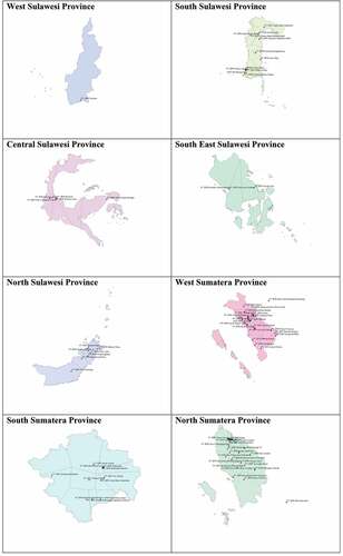
The market boundary (BOUNDARY) is constructed using Thiessen polygons. A Thiessen polygon is a geometrical approach. The boundaries in this polygon define the area closest to each point relative to all other points (have the same distance to two centers). These polygons are mathematically described by the perpendicular bisectors of the lines between all points (Brassel & Reif, 1979). I create and calculate the Thiessen polygons using ArcGIS software. First, I assign the latitude and longitude coordinates to each province map in the shp file. Then I compute the area of the Thiessen polygon as a proxy of the market boundary in km squared. Each Thiessen polygon in Figure A1 defines individual areas of influence around each set of points. This study calculates the square meter region in which rural banks operate per province.⁷

I control bank concentration, measured as market concentration, using the Herfindahl Hirschman index (HHI) for industry-specific characteristics. The concentration indices are estimated based on the banks’ share of assets using bank-level data. I also control for specific dummies variables, the FSA Zone, and ownership types.

Next, I control some provincial macroeconomic variables. Provincial inflation (PROV_INF) is expected to affect bank efficiency. Under inflationary conditions, banks might feel less pressure to maintain their inputs and become less efficient. However, when interest rates are high, banks’ opportunity to earn a profit margin is also higher. Using provincial inflation is more appropriate than national inflation, as some provinces have a dominant influence. Inflation is a regional phenomenon because each province has a different economic situation. Another macroeconomic variable is the provincial gross domestic product (PROV_GDP). Higher provincial GDP growth stimulates investment. Thus, the GDP growth rate is expected to positively affect profitability and efficiency (Demirgüç-Kunt & Huizinga, 1999). This study also uses provincial GDP, as the disparities and inequality among Indonesian regions still exist.

3.4. Methodology and Empirical Specifications

This study uses the stochastic frontier approach (SFA) to analyze the rural banks’ efficiency. It estimates a parametric frontier of the best possible practices given a standard cost function. According to Daraio and Simar (2007), using the parametric model is because applying full nonparametric models can suffer from different problems, such as extreme values or outliers. It allows for a random error, which accounts for measurement errors. Output price can be proxied by observable variables but not for marginal cost, as it has to be estimated. The marginal cost can be done by modeling the cost function. To assess banks’ efficiency, I estimate the cost frontier using a translog function following Christensen et al. (1973). Competition among banks as high regulatory institutions and low innovation (in this study, rural banks) is mainly cost-driven. Thus, modeling the cost function rather than the profit function is generally considered more appropriate. The assumptions of the cost function based on Evans and Heckman (1984) are non-negative and continuous, linear homogenous in the input prices, monotonically increasing in both input prices and outputs, and show concavity in the input prices.

Cost efficiency is the ratio of the minimum cost to a given production volume. Cost efficiency considers a bank inefficient if its prices are higher than predicted for an efficient bank producing the same output under the same existing conditions with the difference unexplainable by statistical noise. Specifically, a stochastic cost function model implies that the bank’s observed total cost deviates from the efficient frontier. Efficiency ranges from 0 to 1.

According to the SFA, the general form of cost efficiency takes the following specification:

(6) $T{C}_{it}=f\left(q_{it},p_{it},\beta \right)+\left(V_{it}+U_{it}\right)$(6)

where

TC_it = total costs (expenses) of the bank

q_it is a vector of outputs

p_it is a vector of input prices

β is a vector of other variables

V_it is a random variable that is assumed independent and identically distributed, with a mean zero

U_it is inefficiency.

It is independently distributed as truncations at zero of the $N\left(m_{it},{\sigma }_U^2\right)$ distribution.

The general form of translog frontier analysis is shown as the equation:

(7) $ln\left(T{C}_i\right)={\beta }_0+\sum \frac{1}{2}{\beta }_i{\left(ln\left(Y_i\right)\right)}^2+\sum \frac{1}{2}{\beta }_j{\left(ln\left(W_j\right)\right)}^2+\sum \sum {\beta }_{ij}ln\left(Y_i\right)ln\left(W_j\right)+V_i+U_i$(7)

where TC_i is total cost; Y_i is output variables; W_j is input price; V_i is a random error; and U_i is cost inefficiency.

This paper selects the translog cost function, reflecting the interaction between explanatory and explained variables. Following Liadaki and Gaganis (2010), a simple way to impose the homogeneity constraints is to normalize all the variables in the translog equation. Thus, I normalize the cost function with one of the input prices. The model is written as follows:

(8) $ln\frac{TC}{P_3}={\beta }_0+{\beta }_{1}ln(Q_1)+{\beta }_{2}ln(Q_2)+{\beta }_{3}ln(Q_3)+{\beta }_{4}ln\left(\frac{P_1}{P_3}\right)+{\beta }_{5}ln\left(\frac{P_2}{P_3}\right)+{\beta }_6\frac{1}{2}{[ln(Q_1)]}^2+{\beta }_{7}ln(Q_1)ln(Q_2)+{\beta }_{8}ln(Q_1)ln(Q_3)+{\beta }_9\frac{1}{2}{[ln(Q_2)]}^2+{\beta }_{10}ln(Q_2)ln(Q_3)+{\beta }_{11}\frac{1}{2}{[ln(Q_3)]}^2+{\beta }_{12}\frac{1}{2}{\left[ln\left(\frac{P_1}{P_3}\right)\right]}^2+{\beta }_{13}ln\left(\frac{P_1}{P_3}\right)ln\left(\frac{P_2}{P_3}\right)+{\beta }_{14}\frac{1}{2}{\left[ln\left(\frac{P_2}{P_3}\right)\right]}^2+{\beta }_{15}ln(Q_1)ln\left(\frac{P_1}{P_3}\right)+{\beta }_{16}ln(Q_1)ln\left(\frac{P_2}{P_3}\right)+{\beta }_{17}ln(Q_2)ln\left(\frac{P_1}{P_3}\right)+{\beta }_{18}ln(Q_2)ln\left(\frac{P_2}{P_3}\right)+{\beta }_{19}ln(Q_3)ln\left(\frac{P_1}{P_3}\right)+{\beta }_{20}ln(Q_3)ln\left(\frac{P_2}{P_3}\right)+(V_{it}+U_{it})$(8)

where TC is defined as the total costs, P_i is the vector of input prices; Q_i is a vector of variable outputs. This model is estimated using a stochastic frontier model. To calculate the level of cost efficiency, based on Battese and Coelli (1992), I use the ratio of the observed cost relative to the potential cost, defined by:

(9) $CostInefficienc{y}_{it}=\frac{C_{it}^{\ast }}{C_{it}}=\frac{exp\left(x_{it}\beta \right)}{exp\left(x_{it}\beta +u_{it}\right)}=exp\left(-u_{it}\right)$(9)

(10) $Efficienc{y}_{it}=1-exp\left(-u_{it}\right)$(10)

The cost efficiency model for SFA could be expanded with netput variables and other control variables, as follows:

(11) $T{C}_{it}=f\left(Q_{it},P_{it},N_{it}\right)+v_{it}+u_{it}$(11)

Where $T{C}_{it}$ stands for the total cost of bank i at time t, $Q_{it}$ is a vector of inputs, $P_{it}$ is a vector of outputs, $N_{it}$ is a vector of quasi-fixed netputs, $v_{it}$ stands for the random variables, which are assumed independent and identically distributed, with mean zero and constant variance and independent of the $u_{it}$ as inefficiency (non-negative random variables). Following Battese and Coelli (1995), the error is distributed as truncations at zero of the $N\left(m_{it},{\sigma }_u^2\right)$ distribution, where the mean, $m_{it}$, is assigned as $m_{it}=z_{it}\delta$, where $z_{it}$ is a vector of variances that affect the efficiency, and $\delta$ is the vector with the parameters to be estimated. This study includes quasi-fixed netput, the fixed assets of each bank (N1). Furthermore, equity (N2) is a second quasi-fixed netput representing an alternative funding source for banks. Therefore, it might affect their cost structure (Fiordelisi et al., 2011).

The translog cost function is constructed as follows:

(12) $ln{TC}_{it}={\alpha }_0+\sum _i{\alpha }_{i}ln{Q}_{it}+\sum _i{\beta }_{i}ln{P}_{it}+\sum _i\zeta ln{N}_{it}+\frac{1}{2}\sum _i\sum _j{\alpha }_{i}ln{Q}_{it}ln{Q}_{jt}+\frac{1}{2}\sum _i\sum _j{\beta }_{i}ln{P}_{it}ln{P}_{jt}+\frac{1}{2}\sum _i\sum _j{\zeta }_{i}ln{N}_{it}ln{N}_{jt}+\sum _i\sum _j{\delta }_{ij}ln{Q}_{it}ln{P}_{jt}+\frac{1}{2}\sum _i\sum _j{\theta }_{i}ln{Q}_{it}ln{N}_{jt}+\sum _i\sum _j{k}_{ij}ln{P}_{it}ln{N}_{jt}+v_{it}+u_{it}$(12)

(13) $ln\frac{TC}{P_3}={\beta }_0+{\beta }_{1}ln(Q_1)+{\beta }_{2}ln(Q_2)+{\beta }_{3}ln(Q_3)+{\beta }_{4}ln(N_1)+{\beta }_{5}ln(N_2)+{\beta }_{6}ln\left(\frac{P_1}{P_3}\right)+{\beta }_{7}ln\left(\frac{P_2}{P_3}\right)+{\beta }_8\frac{1}{2}{[ln(Q_1)]}^2+{\beta }_{9}ln(Q_1)ln(Q_2)+{\beta }_{10}ln(Q_1)ln(Q_3)+{\beta }_{11}12{[ln(Q_2)]}^2+{\beta }_{12}ln(Q_2)ln(Q_3)+{\beta }_{13}\frac{1}{2}{[ln(Q_3)]}^2+{\beta }_{14}12{[ln(N_1)]}^2+{\beta }_{15}ln(N_1)ln(N_2)+{\beta }_{16}12{[ln(N_2)]}^2+{\beta }_{17}\frac{1}{2}{\left[ln\left(\frac{P_1}{P_3}\right)\right]}^2+{\beta }_{18}ln\left(\frac{P_1}{P_3}\right)ln\left(\frac{P_2}{P_3}\right)+{\beta }_{19}\frac{1}{2}{\left[ln\left(\frac{P_2}{P_3}\right)\right]}^2+{\beta }_{20}ln(Q_1)ln\left(\frac{P_1}{P_3}\right)+{\beta }_{21}ln(Q_1)ln\left(\frac{P_2}{P_3}\right)+{\beta }_{22}ln(Q_2)ln\left(\frac{P_1}{P_3}\right)+{\beta }_{23}ln(Q_2)ln\left(\frac{P_2}{P_3}\right)+{\beta }_{24}ln(Q_3)ln\left(\frac{P_1}{P_3}\right)+{\beta }_{25}ln(Q_3)ln\left(\frac{P_2}{P_3}\right)+{\beta }_{26}ln(N_1)ln\left(\frac{P_1}{P_3}\right)+{\beta }_{27}ln(N_1)ln\left(\frac{P_2}{P_3}\right)+{\beta }_{28}ln(N_2)ln\left(\frac{P_1}{P_3}\right)+{\beta }_{29}ln(N_2)ln\left(\frac{P_2}{P_3}\right)+{\beta }_{30}ln(N_1)ln(Q_1)+{\beta }_{31}ln(N_1)ln(Q_2)+{\beta }_{32}ln(N_1)ln(Q_3)+{\beta }_{33}ln(N_2)ln(Q_1)+{\beta }_{34}ln(N_2)ln(Q_2)+{\beta }_{35}ln(N_2)ln(Q_3)+(V_{it}+U_{it})$(13)

Hence, the inefficiency, $U_{it}$, is obtained by truncation of the normal distribution with mean, $m_{it}=z_{it}\delta$. It takes the following form:

(14) $m_{it}={\delta }_0+{\delta }_{1}SpatialCompetitio{n}_{it}+{\delta }_{2}HH{I}_{it}+{\delta }_{3}GD{P}_{jt}+{\delta }_{4}Inflatio{n}_{jt}+{\epsilon }_{it}$(14)

3.5. Descriptive statistics

Table 1 provides a list of variables with symbols and definitions. This table contains summary statistics for the variables employed in analyzing the effect of spatial competition on bank efficiency. There are 20,443 bank-quarter observations in the final sample over the entire period from Q1–2014 to Q4–2018. As I avoid a disturbance by extreme economic conditions, I control the provincial characteristics in the model.

Table 1. Variables definition and summary statistics

Variable	Symbol	Definition	Obs	Mean	St. Dev	Min	Max	P25	P50	P75
Distance	DISTANCE	Distance from bank to nearest rival bank (in meters)	20,443	5,687	14,222	8.91	102,507	478.92	1,212	3,813
Log Natural Distance	LN_DISTANCE	Natural log of distance from bank to a nearest rival bank	20,443	7.131	1.807	2.187	11.538	6.172	7.100	8.246
Boundary	BOUNDARY	Area of Thiessen polygon for each bank (in km squared)	20,443	1,190	4,140	0.224	31,100	9.727	69.5	406
Log Natural Boundary	LN_BOUNDARY	Natural log of the area of Thiessen polygon for each bank	20,443	18.067	2.541	12.322	24.159	16.090	18.056	19.823
HHI	HHI	The market concentration of assets	20,443	1,197.19	1,565.70	155.32	8,405.31	541.23	715.88	1,257.20
Log Natural HHI	LN_HHI	Natural log of market concentration of assets	20,443	6.585	0.977	5.045	9.037	6.294	6.574	7.137
GDP	PROV_GDP	Growth of provincial GDP by Expenditures in Constant Prices	20,443	0.054	0.010	−0.001	0.084	0.052	0.054	0.059
Inflation	PROV_INF	Provincial Inflation	20,443	0.043	0.038	−0.041	0.179	0.023	0.040	0.056
Total Assets	Y	Total Assets (billion rupiah)	20,443	53.6	92.3	1.961	602	11.6	22.5	49
Price	P	Total revenues to total assets	20,443	0.367	0.125	0.167	0.757	0.277	0.343	0.430
Total Cost	TC	Total Interest Expenses + Total Operational Expenses (billion rupiah)	20,443	15.60	26.00	0.653	174	3.365	6.907	15.5
Outputs:
Loans	$Q_1$	Loans to other rural banks + Loans to commercial banks + Loans to non-bank-related parties + Loans to non-bank-unrelated parties (billion rupiah)	20,443	40.10	70.8	1.305	464	8.221	16.7	36.7
Other earning assets	$Q_2$	Interbank placement (billion rupiah)	20,443	11.4	21.3	0.183	138	1.928	4.367	10.1
Non-interest income	$Q_3$	Non-interest income (billion rupiah)	20,443	0.677	1.160	0.011	7.867	0.125	0.290	0.694
Inputs:
Price of labor	$P_1$	The ratio of administrative expenses to total assets	20,443	0.106	0.052	0.023	0.276	0.068	0.097	0.134
Price of physical capital	$P_2$	The ratio of depreciation expenses to fixed assets	20,443	0.606	0.186	0.135	0.924	0.481	0.619	0.754
Price of borrowed funds	$P_3$	The ratio of interest expenses to total deposits	20,443	0.095	0.044	0.034	0.292	0.069	0.086	0.106
Netput 1	$N_1$	Fixed assets (billion rupiah)	20,443	0.914	1.666	0.014	10.7	0.160	0.344	0.818
Netput 2	$N_2$	Equity (billion rupiah)	20,443	8.806	13.6	0.516	89.7	2.526	4.482	8.509

This table presents the definition of all variables and their summary statistics. The sample covers all Indonesian rural banks from 2014:Q1 to 2018:Q4. All financial ratios are winsorized at a 1 percent level on the top and bottom of the distribution. I also annualized all financial variables. All level financial variables are denominated in billions of Indonesian rupiah (IDR), deflated using the 2014 Consumer Price Index (CPI) deflator.

Regarding input prices, the highest value is the price of physical capital (60.56 percent), among other input prices, price of labor, and price of funds, which are 10.6 and 9.5 percent, respectively.⁸ As found in many previous studies, the physical capital expenses (depreciation and occupancy expenses) to fixed assets are mostly high, as banks spend many of their sources on building, inventory, and equipment.

Rural banks have less than 2 percent of total assets compared with commercial banks. Thus, rural banks have a relatively small market share in the industry. However, even though rural banks have only less than two percent of the total asset compared to commercial banks, they have a significant role in the Indonesian banking system as IDIC guarantees their deposits. However, they have high-interest rates to compensate for their risk, as they provide services mostly to local economies or opaque businesses.⁹ Thus, these banks require more return on assets than commercial banks, around 3 percent. This implication can be seen as a potential adverse selection in the financial system. It can occur when opaque or risky borrowers are likely to produce an undesirable outcome (then create a non-performing loan). Capital adequacy is measured by the ratio of capital, the sum of a bank’s Tier 1 (core capital and includes disclosed reserves) to total assets. The minimum of this ratio is 8 percent. Indonesia’s Financial Services Authority (Otoritas Jasa Keuangan/OJK) determines the core capital level to open the bank according to bank classification and risk profile (FSA Zone) under Regulation No. 20/POJK.03/2014.

It is turning to the main variables of interest, the spatial variables: distance from a bank to the closest rival bank and market boundary. I observe that the median of the distance in the sample is 1,212 m, and the nearest distance between a bank and its rival bank is about six kilometers (5,687 m) located in the same province. Another variable of interest, the boundary (the meter square of the polygon area for each bank), has 1,190 m squared, on average, as the boundary. It shows that the distance between banks is close enough to each other. This geographic factor is relevant when studying the rural banking market, despite new technology that might have suggested otherwise (Brevoort & Hannan, 2006). The data on bank location is collected from Bank Indonesia, and the addresses of the FSA office in each province are also collected to build excluded instruments for IV estimation (see the endogeneity section). Finally, the data on the population at the provincial level are taken from the Indonesian Central Bureau of Statistics.

Part of this study’s theoretical motivation relates to measuring market concentration. Hence, I construct a measure of market concentration using the HHI, reflecting the market differentiation degree and its monopoly. The average HHI of rural banks is 1,197 during the sample period, which is moderately concentrated. Similar to some findings for ASEAN countries (see Nguyen T.L.A, 2018 and Rao Subramaniam, V. P., 2019). The rural banking market per province tends to be more concentrated in a larger boundary. It also highlights the range of variation within provinces, where the maximum HHI exceeds 8,000 and 155 for the minimum. Moreover, it shows small variability and less monopoly power for the Indonesian rural banking sector.

Turning to the macroeconomics variables, the average provincial GDP and inflation growth rate reflecting each province’s economic environment shows 5.41 percent and 4.27 percent, respectively. However, it varies considerably across provinces. The GDP ranges from the lowest, −0.1 percent, to the highest, 8.4 percent. In contrast to the GDP growth rate, inflation seems much more volatile across provinces, ranging from−4.1 percent and 17.9 percent. These relatively high numbers show that Indonesia is an emerging market with high growth expectations.

Next, I include ownership types and FSA Zone dummies to reflect empirical findings of the existing literature. Specifically, rural banks are distinguished by three ownership types: 1) public/state ownership, 2) privately owned, and 3) cooperative. Based on FSA regulation, there are four zones based on economic potential and level of banking competition in a region. The rural banks are mostly privately owned and established in Zone 2, requiring a minimum capital of IDR 8 billion (approximately USD 570,000).

I also report a correlation matrix for the independent variables. Table 2 presents the pairwise correlation coefficients. As shown from the table, there is no correlation between each independent variable above 70 percent (strong linear correlation). Thus, the independent variables do not suffer from multicollinearity problems (Gujarati & Porter, 2004). However, the correlations are significant at the 1 percent level.

Table 2. Correlation matrix

	DISTANCE	BOUNDARY	W1	W2	W3	LERNER	MC	HHI	PROV_GDP	PROV_INF
DISTANCE	1
BOUNDARY	0.63^a	1
W1	0.07^a	0.14^a	1
W2	−0.05^a	0.01^a	0.27^a	1
W3	−0.06 ^a	−0.17^a	−0.09^a	−0.08^a	1
LERNER	−0.03^a	0.05^a	0.02^a	0.02^b	−0.16^a	1
MC	0.05^a	0.02^a	0.38^a	0.10^a	0.18^a	−0.84^a	1
HHI	0.20^a	0.30^a	0.08^a	0.01^a	0.03^a	−0.03^a	0.06^a	1
PROV_GDP	−0.07^a	−0.19^a	−0.04^a	0.00^a	0.13^a	−0.05^a	0.04^a	0.03^a	1
PROV_INF	0.03^a	0.01^a	0.03^a	−0.00^a	0.04^a	−0.40^a	0.39^a	0.04^a	0.05^a	1

^asignificant at 1 percent level

^bsignificant at 5 percent level

^csignificant at 10 percent level

This table presents the pairwise correlation between independent variables. The sample covers all Indonesian rural banks from 2014:Q1 to 2018:Q4. All financial ratios are winsorized at the 1 percent level on the top and bottom of the distribution. I also annualized all financial variables. All level financial variables are denominated in billions of Indonesian rupiah (IDR), deflated using the 2014 Consumer Price Index (CPI) deflator.

4. Empirical results and analysis

4.1. The effect of spatial competition on bank efficiency

The cost efficiency is measured using the parametric approach, SFA. To assess banks’ cost efficiency, I estimate the cost frontier using a translog function as in Eq. (12)(12) $ln{TC}_{it}={\alpha }_0+\sum _i{\alpha }_{i}ln{Q}_{it}+\sum _i{\beta }_{i}ln{P}_{it}+\sum _i\zeta ln{N}_{it}+\frac{1}{2}\sum _i\sum _j{\alpha }_{i}ln{Q}_{it}ln{Q}_{jt}+\frac{1}{2}\sum _i\sum _j{\beta }_{i}ln{P}_{it}ln{P}_{jt}+\frac{1}{2}\sum _i\sum _j{\zeta }_{i}ln{N}_{it}ln{N}_{jt}+\sum _i\sum _j{\delta }_{ij}ln{Q}_{it}ln{P}_{jt}+\frac{1}{2}\sum _i\sum _j{\theta }_{i}ln{Q}_{it}ln{N}_{jt}+\sum _i\sum _j{k}_{ij}ln{P}_{it}ln{N}_{jt}+v_{it}+u_{it}$(12) . This study uses the Battese and Coelli (1995) model as the baseline. Next, I run the SFA model using sfpanel produced by Belotti et al. (2015). As noted in their study, sfpanel is designed to estimate SFA models using panel data and allows a broader range of time-varying inefficiency models compared with the xtfrontier command. The estimation of the effect of spatial competition on bank efficiency is shown in Table 3. The average cost efficiency in the sample is 82.43 percent, with a minimum efficiency score of 79.03 percent and a maximum of 86.31 percent. Finally, I run the mean of inefficiency, which includes distance. The coefficient of distance is a positive 0.0294 and statistically significant at 1 percent. All mean variables are significant except for GDP growth and ownership types dummy. The insignificant effect of bank ownership on bank efficiency is against Antunes et al. (2022), which found that state-owned banks have the highest efficiency.

Table 3. Stochastic Frontier Analysis (SFA) estimation using distance as a spatial variable

$\mathit{l}n\frac{TC}{W_3}$	Coefficient		Coefficient
Frontier
$ln\left(Q_1\right)$	0.9984*** (10.60)	$ln\left(Q_1\right)ln\left(\frac{P_1}{P_3}\right)$	−0.0264* (−1.84)
$ln\left(Q_2\right)$	0.5161*** (9.08)	$ln\left(Q_1\right)ln\left(\frac{P_2}{P_3}\right)$	0.0507*** (3.13)
$ln\left(Q_3\right)$	−0.0586 (−1.42)	$ln\left(Q_2\right)ln\left(\frac{P_1}{P_3}\right)$	−0.0379*** (4.39)
$ln\left(N_1\right)$	0.1913*** (3.50)	$ln\left(Q_2\right)ln\left(\frac{P_2}{P_3}\right)$	0.0050 (0.46)
$ln\left(N_2\right)$	−0.4120*** (−5.45)	$ln\left(Q_3\right)ln\left(\frac{P_1}{P_3}\right)$	−0.0082 (−1.30)
$ln\left(\frac{P_1}{P_3}\right)$	1.096*** (9.68)	$ln\left(Q_3\right)ln\left(\frac{P_2}{P_3}\right)$	0.0124* (1.70)
$ln\left(\frac{P_2}{P_3}\right)$	0.6247*** (5.22)	$ln\left(N_1\right)ln\left(\frac{P_1}{P_3}\right)$	−0.0037 (−0.36)
$\frac{1}{2}{\left[ln\left(Q_1\right)\right]}^2$	0.0839*** (5.50)	$ln\left(N_1\right)ln\left(\frac{P_2}{P_3}\right)$	−0.1150*** (−8.59)
$ln\left(Q_1\right)ln\left(Q_2\right)$	−0.1867*** (−25.77)	$ln\left(N_2\right)ln\left(\frac{P_1}{P_3}\right)$	0.0554*** (4.81)
$ln\left(Q_1\right)ln\left(Q_3\right)$	−0.0009 (−0.18)	$ln\left(N_2\right)ln\left(\frac{P_2}{P_3}\right)$	0.018 (1.28)
$\frac{1}{2}{\left[ln\left(Q_2\right)\right]}^2$	0.1433*** (24.38)	$ln\left(N_1\right)ln\left(Q_1\right)$	−0.0214*** (−2.81)
$ln\left(Q_2\right)ln\left(Q_3\right)$	0.0037 (1.09)	$ln\left(N_1\right)ln\left(Q_2\right)$	0.0144*** (2.94)
$\frac{1}{2}{\left[ln\left(Q_3\right)\right]}^2$	0.0017 (0.50)	$ln\left(N_1\right)ln\left(Q_3\right)$	0.0003 (0.11)
$\frac{1}{2}{\left[ln\left(N_1\right)\right]}^2$	−0.0088 (−1.26)	$ln\left(N_2\right)ln\left(Q_1\right)$	0.0956*** (8.94)
$ln\left(N_1\right)ln\left(N_2\right)$	0.0227*** (3.77)
$\frac{1}{2}{\left[ln\left(N_2\right)\right]}^2$	−0.1315*** (−11.59)	$ln\left(N_2\right)ln\left(Q_2\right)$	0.0256*** (4.41)
$\frac{1}{2}{\left[ln\left(\frac{P_1}{P_3}\right)\right]}^2$	0.2370*** (10.40)	$ln\left(N_2\right)ln\left(Q_3\right)$	−0.0007 (−0.18)
$ln\left(\frac{P_1}{P_3}\right)ln\left(\frac{P_2}{P_3}\right)$	−0.1202*** (−5.31)	constant	−0.6114 (−1.30)
$\frac{1}{2}{\left[ln\left(\frac{P_2}{P_3}\right)\right]}^2$	−0.1662*** (5.49)
Mu
DISTANCE	0.0294*** (4.98)
HHI	0.12998*** (12.01)
PROV_GDP	1.2416 (1.42)
PROV_INF	11.42*** (42.07)
ZONE1	0.3069*** (7.11)
ZONE2	0.1986*** (5.84)
ZONE3	0.2044*** (5.14)
STATE	0.0956 (1.14)
PRIVATE	0.0649 (0.82)
Constant	−1.6184 (−12.01)
Cost-efficiency	Mean 0.8243	Min 0.7903	Max 0.8631

This table presents the SFA estimation of bank cost efficiency using distance as a spatial variable. ***, **, * indicate significance at the 1 percent, 5 percent, and 10 percent levels, respectively. The numbers in parentheses are t-statistics.

Then, I also run the model, which includes the boundary in the mean equation, as shown in Table 4. The coefficient is−0.0193 and significant at 1 percent. All of the variables show consistent results with the previous one. The negative coefficient of the exogenous variable in the regression indicates that banks with larger values of the variables tend to have a lower level of inefficiency (they are more efficient). It means that distance has a negative effect on bank efficiency.

Table 4. Stochastic Frontier Analysis (SFA) estimation using boundary as a spatial variable

$\mathit{l}n\frac{TC}{W_3}$	Coefficient		Coefficient
Frontier
$ln\left(Q_1\right)$	1.0012*** (10.64)	$ln\left(Q_1\right)ln\left(\frac{P_1}{P_3}\right)$	−0.0246* (−1.72)
$ln\left(Q_2\right)$	0.5103*** (8.97)	$ln\left(Q_1\right)ln\left(\frac{P_2}{P_3}\right)$	0.0496*** (3.06)
$ln\left(Q_3\right)$	−0.0612 (−1.48)	$ln\left(Q_2\right)ln\left(\frac{P_1}{P_3}\right)$	−0.0371*** (−4.30)
$ln\left(N_1\right)$	0.1926*** (3.52)	$ln\left(Q_2\right)ln\left(\frac{P_2}{P_3}\right)$	0.0058 (0.53)
$ln\left(N_2\right)$	−0.4006*** (−5.30)	$ln\left(Q_3\right)ln\left(\frac{P_1}{P_3}\right)$	−0.0092 (−1.46)
$ln\left(\frac{P_1}{P_3}\right)$	1.1001*** (9.72)	$ln\left(Q_3\right)ln\left(\frac{P_2}{P_3}\right)$	0.0130* (1.77)
$ln\left(\frac{P_2}{P_3}\right)$	0.6154*** (5.14)	$ln\left(N_1\right)ln\left(\frac{P_1}{P_3}\right)$	−0.0032 (−0.31)
$\frac{1}{2}{\left[ln\left(Q_1\right)\right]}^2$	0.0852*** (5.60)	$ln\left(N_1\right)ln\left(\frac{P_2}{P_3}\right)$	−0.1167*** (−8.69)
$ln\left(Q_1\right)ln\left(Q_2\right)$	−0.1864*** (−25.74)	$ln\left(N_2\right)ln\left(\frac{P_1}{P_3}\right)$	0.0527*** (4.59)
$ln\left(Q_1\right)ln\left(Q_3\right)$	−0.0009 (−0.17)	$ln\left(N_2\right)ln\left(\frac{P_2}{P_3}\right)$	0.0203 (1.44)
$\frac{1}{2}{\left[ln\left(Q_2\right)\right]}^2$	0.1431*** (24.35)	$ln\left(N_1\right)ln\left(Q_1\right)$	−0.0210*** (−2.76)
$ln\left(Q_2\right)ln\left(Q_3\right)$	0.0036 (1.06)	$ln\left(N_1\right)ln\left(Q_2\right)$	0.0147*** (2.99)
$\frac{1}{2}{\left[ln\left(Q_3\right)\right]}^2$	0.0015 (0.47)	$ln\left(N_1\right)ln\left(Q_3\right)$	0.0003 (0.11)
$\frac{1}{2}{\left[ln\left(N_1\right)\right]}^2$	−0.0098 (−1.41)	$ln\left(N_2\right)ln\left(Q_1\right)$	0.0936*** (8.78)
$ln\left(N_1\right)ln\left(N_2\right)$	0.0231*** (3.82)	$ln\left(N_2\right)ln\left(Q_2\right)$	0.0256*** (4.41)
$\frac{1}{2}{\left[ln\left(N_2\right)\right]}^2$	−0.1308*** (−11.55)	$ln\left(N_2\right)ln\left(Q_3\right)$	−0.0005 (−0.12)
$\frac{1}{2}{\left[ln\left(\frac{P_1}{P_3}\right)\right]}^2$	0.2376*** (10.43)	constant	−0.6670 (−1.41)
$ln\left(\frac{P_1}{P_3}\right)ln\left(\frac{P_2}{P_3}\right)$	−0.1183*** (5.22)
$\frac{1}{2}{\left[ln\left(\frac{P_2}{P_3}\right)\right]}^2$	−0.1697*** (−5.60)
Mu
BOUNDARY	−0.0193*** (−4.26)
HHI	0.1376*** (12.60)
PROV_GDP	0.6310 (0.71)
PROV_INF	11.48*** (42.09)
ZONE1	0.1523*** (3.31)
ZONE2	0.0611* (1.73)
ZONE3	0.1202*** (2.98)
STATE	0.1026 (1.22)
PRIVATE	0.0362 (0.45)
Constant	−1.4143 (−10.26)
Cost-efficiency	Mean 0.8195	Min 0.7872	Max 0.8593

This table presents the SFA estimation of bank cost efficiency using boundary as a spatial variable. ***, **, * indicate significance at the 1 percent, 5 percent, and 10 percent levels, respectively. The numbers in parentheses are t-statistics.

On the other hand, the boundary positively affects bank efficiency. The possible explanation is since rural banks face the lower competition of new entrants as they can only open a business in their province, this less openness could be associated with a lower degree of contestability. In addition, the HHI also shows that a more concentrated market (less competition) results in inefficiency. These results support the argument that more concentrated markets tend to be more collusive, and banks earn monopolistic profits, aligning with the SCP paradigm (Lloyd-Williams et al., 1994). The results of HHI are also consistent with some previous research. For instance, Vinh (2017) examines the effect of concentration on the Vietnamese banking sector from 2005 to 2015 and finds that the HHI effect on profit is significantly positive at a 5 percent level. Khan et al. (2018) also conclude that higher profits are found in a concentrated market. In a study by Ho and Ishii (2011), consumers prefer closer banks. Thus, when banks are more distant from other banks, the consumer will choose the closest one, as interest rates on small business loans increase the distance between borrowers and lenders (Belluci et al., 2013). In this respect, the results support the positive impact of competition on efficiency, which aligns with C. F. Chen’s (2007) findings and Dick and Lehnert’s (2010)

4.2. Endogeneity in SFA model

The SFA model can lead to endogeneity issues. One of the concerns is the maximum likelihood estimation, which gives inconsistent parameter estimates (Greene, 2005). I address this problem by following the recent work of Karakaplan and Kutlu (2017), which can treat the endogeneity of frontier and inefficiency variables. Using this method will result in more robust estimations. This model needs instrumental variables (IVs) to address the endogeneity issue.

As noted in some previous frontier models, I also include variables that capture differences across ownership types and groups (FSA Zone) and use the netputs of equity and fixed assets (Hughes & Mester, 1993). Heterogeneity can lead to poor estimates of banks’ efficiency, so I include these variables, as I know that a standard benchmark of a single cost function cannot be used (Mester, 1997).

I conducted the model using the xtsfkk command in STATA (Karakaplan & Kutlu, 2017) and used the BC95 model. I still utilize the translog cost function with three input prices (the price of labor, the price of physical capital, and the price of funds), three outputs (loan, other earning assets, and non-interest income), and two netputs (fixed assets and equity). The estimation results are shown in Table 5. There are two models presented, the EX and EN model. Model EX ignores endogeneity, while Model EN handles endogeneity. HHI and spatial competition variables are endogenous in this model. As I find in the previous results, the HHI has a positive effect on cost inefficiency, and it is statistically significant, which agrees with the quiet life hypothesis and against with Yin (2021)

Table 5. Endogenous Panel Stochastic Frontier Analysis (SFA) using distance as a spatial variable

Dependent Variable: $ln\frac{TC}{W_3}$	Model EX	Model EN
$ln\left(Q_1\right)$	0.395* (0.200)	0.397 (0.230)
$ln\left(Q_2\right)$	0.288* (0.119)	0.275* (0.126)
$ln\left(Q_3\right)$	0.145 (0.089)	0.145 (0.092)
$ln\left(N_1\right)$	0.160 (0.123)	0.176 (0.134)
$ln\left(N_2\right)$	−0.070 (0.174)	−0.064 (0.195)
$ln\left(\frac{P_1}{P_3}\right)$	1.003*** (0.259)	0.991*** (0.275)
$ln\left(\frac{P_2}{P_3}\right)$	0.861*** (0.254)	0.872** (0.266)
$\frac{1}{2}{\left[ln\left(Q_1\right)\right]}^2$	0.130*** (0.028)	0.133*** (0.037)
$ln\left(Q_1\right)ln\left(Q_2\right)$	−0.138*** (0.015)	−0.138*** (0.018)
$ln\left(Q_1\right)ln\left(Q_3\right)$	−0.017 (0.011)	−0.018 (0.012)
$\frac{1}{2}{\left[ln\left(Q_2\right)\right]}^2$	0.124*** (0.013)	0.124*** (0.013)
$ln\left(Q_2\right)ln\left(Q_3\right)$	0.000 (0.007)	−0.001 (0.007)
$\frac{1}{2}{\left[ln\left(Q_3\right)\right]}^2$	0.004 (0.007)	0.006 (0.007)
$\frac{1}{2}{\left[ln\left(N_1\right)\right]}^2$	0.008 (0.015)	0.007 (0.016)
$ln\left(N_1\right)ln\left(N_2\right)$	0.024 (0.013)	0.023 (0.015)
$\frac{1}{2}{\left[ln\left(N_2\right)\right]}^2$	−0.105*** (0.026)	−0.103** (0.036)
$\frac{1}{2}{\left[ln\left(\frac{P_1}{P_3}\right)\right]}^2$	0.1999*** (0.055)	0.205*** (0.057)
$ln\left(\frac{P_1}{P_3}\right)ln\left(\frac{P_2}{P_3}\right)$	−0.120* (0.052)	−0.121* (0.054)
$\frac{1}{2}{\left[ln\left(\frac{P_2}{P_3}\right)\right]}^2$	0.015 (0.060)	0.010 (0.062)
$ln\left(Q_1\right)ln\left(\frac{P_1}{P_3}\right)$	−0.009 (0.032)	−0.004 (0.037)
$ln\left(Q_1\right)ln\left(\frac{P_2}{P_3}\right)$	0.084* (0.034)	0.079* (0.040)
$ln\left(Q_2\right)ln\left(\frac{P_1}{P_3}\right)$	−0.036 (0.020)	−0.037 (0.021)
$ln\left(Q_2\right)ln\left(\frac{P_2}{P_3}\right)$	−0.060** (0.022)	−0.057* (0.023)
$ln\left(Q_3\right)ln\left(\frac{P_1}{P_3}\right)$	−0.019 (0.014)	−0.022 (0.015)
$ln\left(Q_3\right)ln\left(\frac{P_2}{P_3}\right)$	0.010 (0.016)	0.012 (0.016)
$ln\left(N_1\right)ln\left(\frac{P_1}{P_3}\right)$	−0.007 (0.024)	−0.008 (0.026)
$ln\left(N_1\right)ln\left(\frac{P_2}{P_3}\right)$	−0.060* (0.028)	−0.062* (0.029)
$ln\left(N_2\right)ln\left(\frac{P_1}{P_3}\right)$	0.048 (0.026)	0.047 (0.031)
$ln\left(N_2\right)ln\left(\frac{P_2}{P_3}\right)$	−0.036 (0.030)	−0.034 (0.034)
$ln\left(N_1\right)ln\left(Q_1\right)$	−0.026 (0.016)	−0.027 (0.019)
$ln\left(N_1\right)ln\left(Q_2\right)$	−0.007 (0.011)	−0.006 (0.011)
$ln\left(N_1\right)ln\left(Q_3\right)$	0.008 (0.007)	0.008 (0.008)
$ln\left(N_2\right)ln\left(Q_1\right)$	0.045* (0.023)	0.043 (0.035)
$ln\left(N_2\right)ln\left(Q_2\right)$	0.036** (0.012)	0.037** (0.014)
$ln\left(N_2\right)ln\left(Q_3\right)$	0.002 (0.010)	0.002 (0.010)
constant	9.918*** (1.088)
Mu
DISTANCE	0.115*** (0.035)	0.002 (0.042)
HHI	0.252*** (0.056)	0.115 (0.066)
PROV_GDP	−1.922 (3.466)	−2.530 (3.558)
PROV_INF	23.710*** (0.798)	23.756*** (0.806)
ZONE1	0.739** (0.229)	0.386 (0.234)
ZONE2	0.148 (0.180)	−0.225 (0.189)
ZONE3	−0.038 (0.227)	−0.363 (0.232)
STATE	0.436 (0.503)	0.461 (0.498)
PRIVATE	0.147 (0.479)	0.113 (0.475)
Constant	−6.655*** (0.673)
Endogenous Variables
HHI	0.026*** (0.007)	0.026*** (0.007)
DISTANCE	0.017*** (0.004)	0.017*** (0.004)
Instrumental Variables
DIST_FSA_POP
BOUNDARY_PROVINCE_POP
Mean Cost-Efficiency	0.8662	0.8649
Min Cost-Efficiency	0.7963	0.7821
Max Cost-Efficiency	0.8798	0.8755

This table presents an endogenous SFA estimation of bank cost efficiency using distance as a spatial variable. Instrumental variables are included. Panel A is Model EX, and Panel B is Model EN. ***, **, * indicate significance at the 1 percent, 5 percent, and 10 percent levels, respectively. The numbers in parentheses are standard errors.

Furthermore, it indicates that higher market concentration leads to higher inefficiency. In line with H. Chen and Strathearn (2020), banks avoid market concentration and spatial socioeconomic appears from neighbors’ banks. I use the bank’s distance to FSA per population and boundary ratio to province area per population as the instrumental variables. The inefficiency variables in model BC95 include HHI, spatial competition variable (distance and boundary), macroeconomics variables (provincial GDP growth and inflation), and the dummy FSA Zone and ownership types dummy variables. I argue that using the Batesse Coelli 95 model is efficient because this study directly includes the inefficiency factors rather than using two-step regression. The results confirm a previous Degl’innocenti et al. (2017) study, which shows that the spatial variable (distance) affects bank efficiency. However, they use a fully nonparametric methodology in a sample of the US and UK. The result also agrees with X. Chen and Lu (2021) in term of the effect of GDP on efficiency.

As can be seen from Table 6, the mean cost efficiencies under Model EN are slightly less than Model EX, as it handles the heterogeneity and endogeneity problems (Karakaplan & Kutlu, 2017). According to this model, the mean cost efficiency is 86.49 percent with distance as a spatial variable and 86.77 percent with a boundary as a spatial variable. Based on the results in Table 6, the only significant inefficiency factors are HHI, bank distance, inflation, and a dummy variable for FSA Zone 1. I find that the rural bank market concentration has a negative effect on efficiency. In terms of spatial variables, the distance from the bank to the closest rival has a negative impact on efficiency. A possible explanation is the substitution effect, which creates price rivalry for loans, deposits, and other bank services in the market. The bank may also use its network advantage to get the customer’s information from the rival bank. Rural banks are generally close to the community, so creditors’ and debtors’ information can be collected easier, especially in districts. The probability of creating a collusive duopoly may also become the reason to extract profits.

Table 6. Endogenous panel stochastic frontier analysis (SFA) using boundary as a spatial variable

Dependent Variable: $ln\frac{TC}{W_3}$	Model EX	Model EN
$ln\left(Q_1\right)$	0.386* (0.197)	0.397 (0.209)
$ln\left(Q_2\right)$	0.279* (0.118)	0.266* (0.121)
$ln\left(Q_3\right)$	0.145 (0.088)	0.150 (0.090)
$ln\left(N_1\right)$	0.163 (0.122)	0.169 (0.128)
$ln\left(N_2\right)$	−0.059 (0.173)	−0.051 (0.181)
$ln\left(\frac{P_1}{P_3}\right)$	0.991*** (0.256)	0.998*** (0.264)
$ln\left(\frac{P_2}{P_3}\right)$	0.848*** (0.252)	0.856*** (0.259)
$\frac{1}{2}{\left[ln\left(Q_1\right)\right]}^2$	0.133*** (0.028)	0.132*** (0.033)
$ln\left(Q_1\right)ln\left(Q_2\right)$	−0.138*** (0.015)	−0.136*** (0.016)
$ln\left(Q_1\right)ln\left(Q_3\right)$	−0.018 (0.011)	−0.018 (0.012)
$\frac{1}{2}{\left[ln\left(Q_2\right)\right]}^2$	0.124*** (0.013)	0.124*** (0.013)
$ln\left(Q_2\right)ln\left(Q_3\right)$	−0.000 (0.007)	−0.001 (0.007)
$\frac{1}{2}{\left[ln\left(Q_3\right)\right]}^2$	0.005 (0.007)	0.005 (0.007)
$\frac{1}{2}{\left[ln\left(N_1\right)\right]}^2$	0.006 (0.015)	0.006 (0.015)
$ln\left(N_1\right)ln\left(N_2\right)$	0.024 (0.013)	0.025 (0.014)
$\frac{1}{2}{\left[ln\left(N_2\right)\right]}^2$	−0.105*** (0.026)	−0.105*** (0.030)
$\frac{1}{2}{\left[ln\left(\frac{P_1}{P_3}\right)\right]}^2$	0.202*** (0.054)	0.207*** (0.056)
$ln\left(\frac{P_1}{P_3}\right)ln\left(\frac{P_2}{P_3}\right)$	−0.117* (0.051)	−0.119* (0.053)
$\frac{1}{2}{\left[ln\left(\frac{P_2}{P_3}\right)\right]}^2$	0.006 (0.060)	0.006 (0.061)
$ln\left(Q_1\right)ln\left(\frac{P_1}{P_3}\right)$	−0.004 (0.032)	−0.001 (0.034)
$ln\left(Q_1\right)ln\left(\frac{P_2}{P_3}\right)$	0.082* (0.034)	0.077* (0.037)
$ln\left(Q_2\right)ln\left(\frac{P_1}{P_3}\right)$	−0.034 (0.020)	−0.035 (0.020)
$ln\left(Q_2\right)ln\left(\frac{P_2}{P_3}\right)$	−0.059** (0.022)	−0.058* (0.023)
$ln\left(Q_3\right)ln\left(\frac{P_1}{P_3}\right)$	−0.023 (0.014)	−0.024 (0.014)
$ln\left(Q_3\right)ln\left(\frac{P_2}{P_3}\right)$	0.012 (0.016)	0.013 (0.016)
$ln\left(N_1\right)ln\left(\frac{P_1}{P_3}\right)$	−0.006 (0.024)	−0.007 (0.025)
$ln\left(N_1\right)ln\left(\frac{P_2}{P_3}\right)$	−0.064* (0.028)	−0.063* (0.029)
$ln\left(N_2\right)ln\left(\frac{P_1}{P_3}\right)$	0.043 (0.026)	0.043 (0.028)
$ln\left(N_2\right)ln\left(\frac{P_2}{P_3}\right)$	−0.031 (0.030)	−0.030 (0.032)
$ln\left(N_1\right)ln\left(Q_1\right)$	−0.026 (0.016)	−0.027 (0.018)
$ln\left(N_1\right)ln\left(Q_2\right)$	−0.006 (0.010)	−0.007 (0.011)
$ln\left(N_1\right)ln\left(Q_3\right)$	0.008 (0.007)	0.008 (0.008)
$ln\left(N_2\right)ln\left(Q_1\right)$	0.043 (0.022)	0.043 (0.029)
$ln\left(N_2\right)ln\left(Q_2\right)$	0.036** (0.012)	0.036** (0.013)
$ln\left(N_2\right)ln\left(Q_3\right)$	0.003 (0.010)	0.002 (0.010)
constant	9.989*** (1.077)	9.882*** (1.110)
Mu
BOUNDARY	−0.059* (0.028)	−0.081** (0.031)
HHI	0.268*** (0.056)	0.138* (0.067)
PROV_GDP	−3.266 (3.528)	−4.297 (3.603)
PROV_INF	24.079*** (0.810)	24.091*** (0.810)
ZONE1	0.242 (0.260)	0.014 (0.270)
ZONE2	−0.272 (0.193)	−0.491* (0.203)
ZONE3	−0.278 (0.232)	−0.514* (0.238)
STATE	0.458 (0.506)	0.455 (0.499)
PRIVATE	0.063 (0.482)	0.055 (0.476)
Constant	9.989*** (1.077)
Endogenous Variables
HHI	0.023*** (0.006)	0.023*** (0.006)
BOUNDARY	0.006* (0.003)	0.006* (0.003)
Instrumental Variables
DIST_FSA_POP
BOUNDARY_PROVINCE_POP
Mean Cost-Efficiency	0.8687	0.8677
Min Cost-Efficiency	0.7932	0.7845
Max Cost-Efficiency	0.8789	0.8774

This table presents an endogenous SFA estimation of bank cost efficiency using boundary as a spatial variable. Instrumental variables are included. Panel A is Model EX, and Panel B is Model EN. ***, **, * indicate significance at the 1 percent, 5 percent, and 10 percent levels, respectively. The numbers in parentheses are standard errors.

Looking at the level of economic development in a province, the characteristics of GDP and inflation are high. The economic condition of the province presumably has less-functioning financial systems than the developed ones. The results show that provincial inflation affects negatively on bank cost efficiency. The results support previous studies concluding that distance (spatial variable) matters in estimating bank profitability (Brevoort & Hannan, 2006; Degl’innocenti et al., 2017).

On the other hand, the boundary positively affects bank efficiency. For example, suppose the bank operates in a wide area or location, in line with the theory of the Hotelling model of spatial competition in Kalnins (2003). In that case, the bank will get more market share, as I assume the number of customers is higher, creating profit. In addition, a less competitive market is expected in the Indonesian rural banking sector mainly because of its remote location, moderated concentrated market structure, and population characteristics. These results are consistent with the results using sfpanel frontier regression. Overall, the results support the competition-efficiency hypothesis. It also helps the idea that banks have mark-up pricing (higher market power) and may choose to reduce their effort to maximize profit (Hicks, 1935).

4.3. Additional analysis: Non-rural banks

To see whether commercial and foreign banks could impact competition in rural banking markets, this study further investigates the effects of big-bank presence on the performance of rural banks. Even though the competition in rural banking is mostly between themselves, competition from other banks may impact rural bank profitability. To assess the effect, I collect data, including the physical addresses of other (non-rural) banks. I calculate the distance of these banks to each rural bank in the sample. Following Cyree and Spurlin (2012), I assess the effect of big bank presence in the rural banking market. The model is shown below

(15) $\begin{array}{rl}& RuralBankEfficiency=f(Distance,BIG\mathrm{\_}Dummy,SpatialCompetition,HHI,\\ & ControlsofBankSpecificCharacteristics,\\ & Provincialmacroeconomics,FSA\mathrm{\_}Zone)\end{array}$(15)

BIG_Dummy is the distance for each nearest commercial or non-rural bank in one province. I assign the dummy variable, BIG_Dummy, to take on the value of 1 if the closest bank to a rural bank is commercial/non-rural and zero otherwise. To instrument the distance variable, which is potentially endogenous, as previously, I use the distance from the bank to the regional FSA office in a province divided by its population.

Table 7 reports that the BIG_Dummy has a negative effect on cost inefficiency which means that the presence of BIG banks affects efficiency positively. However, this effect is not statistically significant. Therefore, I can assume that efficiency is affected by other factors unique to rural banks. My findings suggest a commercial or non-rural bank nearby does not affect rural bank efficiency.

Table 7. Additional analysis (non-rural banks presence) with Stochastic Frontier Analysis (SFA)

$ln\frac{TC}{W_3}$	Coefficient		Coefficient
Frontier
$ln\left(Q_1\right)$	0.9795*** (10.44)	$ln\left(Q_1\right)ln\left(\frac{P_1}{P_3}\right)$	−0.0249* (−1.74)
$ln\left(Q_2\right)$	0.5123*** (9.03)	$ln\left(Q_1\right)ln\left(\frac{P_2}{P_3}\right)$	0.0505*** (3.12)
$ln\left(Q_3\right)$	−0.0559 (−1.36)	$ln\left(Q_2\right)ln\left(\frac{P_1}{P_3}\right)$	−0.0378*** (−4.39)
$ln\left(N_1\right)$	0.2011*** (3.69)	$ln\left(Q_2\right)ln\left(\frac{P_2}{P_3}\right)$	0.0052 (0.47)
$ln\left(N_2\right)$	−0.4078*** (−5.40)	$ln\left(Q_3\right)ln\left(\frac{P_1}{P_3}\right)$	−0.0082 (−1.30)
$ln\left(\frac{P_1}{P_3}\right)$	1.0703*** (9.49)	$ln\left(Q_3\right)ln\left(\frac{P_2}{P_3}\right)$	0.0122* (1.67)
$ln\left(\frac{P_2}{P_3}\right)$	0.6490*** (5.43)	$ln\left(N_1\right)ln\left(\frac{P_1}{P_3}\right)$	−0.0039 (−0.38)
$\frac{1}{2}{\left[ln\left(Q_1\right)\right]}^2$	0.0853*** (5.61)	$ln\left(N_1\right)ln\left(\frac{P_2}{P_3}\right)$	−0.1158*** (−8.65)
$ln\left(Q_1\right)ln\left(Q_2\right)$	−0.1868*** (−25.82)	$ln\left(N_2\right)ln\left(\frac{P_1}{P_3}\right)$	0.0555*** (4.83)
$ln\left(Q_1\right)ln\left(Q_3\right)$	−0.0011 (−0.21)	$ln\left(N_2\right)ln\left(\frac{P_2}{P_3}\right)$	0.0176 (1.25)
$\frac{1}{2}{\left[ln\left(Q_2\right)\right]}^2$	0.1434*** (24.42)	$ln\left(N_1\right)ln\left(Q_1\right)$	−0.0215*** (−2.84)
$ln\left(Q_2\right)ln\left(Q_3\right)$	0.0037 (1.11)	$ln\left(N_1\right)ln\left(Q_2\right)$	0.0145*** (2.96)
$\frac{1}{2}{\left[ln\left(Q_3\right)\right]}^2$	0.0015 (0.46)	$ln\left(N_1\right)ln\left(Q_3\right)$	0.0003 (0.10)
$\frac{1}{2}{\left[ln\left(N_1\right)\right]}^2$ $ln\left(N_1\right)ln\left(N_2\right)$	−0.0088 (−1.27) 0.0224*** (3.72)	$ln\left(N_2\right)ln\left(Q_1\right)$	0.0958*** (8.97)
$\frac{1}{2}{\left[ln\left(N_2\right)\right]}^2$	−0.1319*** (−11.62)	$ln\left(N_2\right)ln\left(Q_2\right)$	0.0257*** (4.43)
$\frac{1}{2}{\left[ln\left(\frac{P_1}{P_3}\right)\right]}^2$	0.2389*** (10.52)	$ln\left(N_2\right)ln\left(Q_3\right)$	−0.0006 (−0.14)
$ln\left(\frac{P_1}{P_3}\right)ln\left(\frac{P_2}{P_3}\right)$	−0.1204*** (−5.33)	constant	−0.5653 (−1.20)
$\frac{1}{2}{\left[ln\left(\frac{P_2}{P_3}\right)\right]}^2$	−0.1688*** (5.57)
Mu
BIG_DUMMY	−0.0225 (−0.88)
DISTANCE	0.0329*** (4.69)
HHI	0.1329*** (11.96)
PROV_GDP	1.199 (1.36)
PROV_INF	11.50*** (41.85)
ZONE1	0.3190*** (7.14)
ZONE2	0.1993*** (5.82)
ZONE3	0.2065*** (5.16)
STATE	0.1078 (1.27)
PRIVATE	0.0802 (0.99)
Constant	−1.656 (−12.13)
Cost-efficiency	Mean 0.8144	Min 0.7870	Max 0.8437

This table presents the SFA estimation of bank cost efficiency on BIG banks’ presence using distance as a spatial variable. ***, **, * indicate significance at the 1 percent, 5 percent, and 10 percent levels, respectively. The numbers in parentheses are t-statistics.

5. Limitations and implications

The limitation of this study is some adjustments to the input prices. For example, the salary account and the employees’ total number are unavailable in the reports, so I change them to general and administration expenses. Furthermore, I use depreciation expenses for physical capital, as the actual material expenditures in the quarterly reports are so high. Regarding the spatial variable, I only use distance from a bank to a rival bank, as the customer’s data or borrower location is not provided. However, I add some additional analysis using commercial and non-rural banks’ distance dummies and see whether their presence can affect rural bank profitability and cost efficiency. To overcome the endogeneity issues, I use distance from a bank to an FSA office divided by its population as an instrumental variable. Furthermore, I include more than 1,000 rural banks as samples; a number is sufficient for the present study.

For the implications of this study, the banking stakeholders (including the policymakers and banking regulators) should be concerned about the location of rural banks because it significantly affects bank efficiency. Moreover, the areas of rural banks are scattered throughout the country. Besides, understanding the degree of competition is helpful in many policy issues. Therefore, policymakers and banking regulators should have a keen eye for the level of banking competition. On the one hand, effective competition between rural banks is essential for local people to reap the benefits (lower prices). Still, on the other hand, imperfect competition may have adverse effects on opaque firms or borrowers. A bank’s performance is affected not only by its characteristics but also by external factors. Location matters in rural banking because people mostly go directly to the bank. Considering the present study’s results, the bank should be located close to other banks but in a broad market area for more cost efficiency.

Nonetheless, further research can be obtained as confirming the results with other rural banking markets is still necessary. The additional spatial variable, such as consumers’ distance from bank branches, may be valuable and exciting to discuss the allocation of costs of bank access between the bank and the consumer. Using a single country in this study but consisting of many provinces, such as Indonesia, rural banking with different provincial characteristics, the methodology of this study can be applied to other banking markets.

6. Conclusion

This paper analyses the importance of physical distance between banks and their closest rival bank and the area or market boundary as a proxy of spatial competition. Using quarterly data of rural banks in Indonesia from Q1-2014 to Q4-2018, I estimate the effect of spatial competition together with bank-specific characteristics, industry-specific characteristics, and macroeconomic variables on bank performance measured by cost efficiency. I use stochastic frontier analysis (SFA) as a parametric approach to estimating cost efficiency. I also include ownership types and FSA Zone as dummy variables. Finally, I handle the endogeneity using model EN in the cost efficiency model.

The result finds that the spatial variable (distance) affects bank efficiency and confirms a previous study by Degl’innocenti et al. (2017). Specifically, the distance from the bank to the closest rival has a negative effect on efficiency, but the boundary positively impacts bank efficiency. Overall, the results support the competition-efficiency hypothesis. In addition, the additional analysis of a commercial or non-rural bank nearby shows no effect on rural bank cost efficiency.

Disclosure statement

No potential conflict of interest was reported by the author.

Notes

1. Bank Indonesia has only released a license for 11 rural banks to issue ATMs.

2. 1 USD = 14,230.80 IDR (as per December 2018).

3. Commonly abbreviated as OJK (Otoritas Jasa Keuangan), an independent institution which has authority to regulate, supervise, examine, and investigate against the activities in the financial services sector established in 2011.

4. These data are available online via the Indonesian Financial Service Authority (Otoritas Jasa keuangan)’s website http://www.ojk.go.id.

5. Commonly abbreviated as BPS (Badan Pusat Statistik), a government institute of Indonesia that is responsible for conducting statistical surveys established in 1960. These data are available online via BPS’s website http://www.bps.go.id.

6. There are two other cost in the rural bank income statement: Marketing expenses and Research and Development expenses. However most of the banks do not put any amount in these accounts. So the effect is mostly zero.

7. I create the boundary using Thiessen polygon for each province as the border. For Java province, for instance, I run the ArcGIS software to get the these polygons for each bank. Thus, the sea and international boundaries are not included in the boundaries, because rural banks can only operate in one province.

8. The price of physical capital of rural banks in Indonesia is relatively high because their characteristic of high depreciation expenses of building and inventory.

9. The average lending rate for rural banks is 20 percent (2018).

APPENDICES

Figure A1. Thiessen Polygons for Each Province in Indonesia.

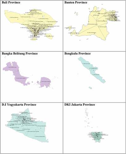
Figure A1. (Continued).

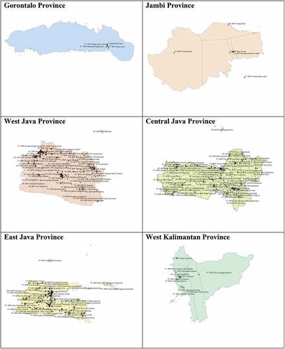
Figure A1. (Continued).

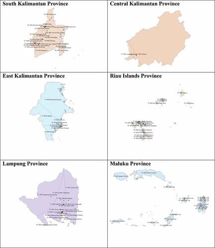
Figure A1. (Continued).

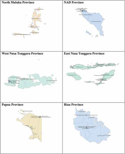
Figure A1. (Continued).

References

- Agarwal, S., & Hauswald, R. (2010). Distance and private information in lending. The Review of Financial Studies, 23(7), 2757–37. https://doi.org/10.1093/rfs/hhq001
- Akhavein, J., Goldberg, L. G., & White, L. J. (2004). Small banks, small business, and relationships: An empirical study of lending to small farms. Journal of Financial Services Research, 26(3), 245–261. https://doi.org/10.1023/B:FINA.0000040051.30624.e2
- Alessandrini, P., Croci, M., & Zazzaro, A. (2009). The geography of banking power: The role of functional distance. In D. Silipo (Ed.), The banks and the Italian economy (pp. 93–123). Physica Springer Berling Heidelberg.
- Alessandrini, P., Presbitero, A. F., & Zazzaro, A. (2008). Banks, distances, and firms’ financing constraints. Review of Finance, 13(2), 261–307. https://doi.org/10.1093/rof/rfn010
- Amel, D. F., & Liang, J. N. (1997). Determinants of entry and profits in local banking markets. Review of Industrial Organization, 12(1), 59–78. https://doi.org/10.1023/A:1007796520286
- Antunes, J., Hadi-Vencheh, A., Jamshidi, A., Tan, Y., & Wanke, P. (2022). Bank efficiency estimation in China: DEA-RENNA approach. Annals of Operations Research, 315(2), 1373–1398. https://doi.org/10.1007/s10479-021-04111-2
- Battese, G. E., & Coelli, T. J. (1992). Frontier production functions, technical efficiency and panel data: With application to paddy farmers in India. Journal of Productivity Analysis, 3(1–2), 153–169. https://doi.org/10.1007/BF00158774
- Battese, G. E., & Coelli, T. J. (1995). A model for technical inefficiency effects in a stochastic frontier production function for panel data. Empirical Economics, 20(2), 325–332. https://doi.org/10.1007/BF01205442
- Bellucci, A., Borisov, A., Giombini, G., & Zazzaro, A. (2019). Collateralization and distance. Journal of Banking & Finance, 100, 205–217.
- Bellucci, A., Borisov, A., & Zazzaro, A. (2013). Do banks price discriminate spatially? Evidence from small business lending in local credit markets. Journal of Banking & Finance, 37(11), 4183–4197. https://doi.org/10.1016/j.jbankfin.2013.06.009
- Bellucci, A., Borisov, A., & Zazzaro, A. (2013). Do banks price discriminate spatially? Evidence from small business lending in local credit markets. Journal of Banking & Finance, 37(11), 4183–4197.
- Belotti, F., Daidone, S., Atella, V., & Ilardi, G. (2015). SFPANEL: Stata module for panel data stochastic frontier models estimation. Statistical Software Components. Boston College Department of Economics.
- Berger, A. N., Demirgüç-Kunt, A., Levine, R., & Haubrich, J. G. (2004). Bank concentration and competition: An evolution in the making. Journal of Money, Credit, and Banking, 36(3b), 433–451. https://doi.org/10.1353/mcb.2004.0040
- Berger, A. N., & Humphrey, D. B. (1997). Efficiency of financial institutions: International survey and directions for future research. European Journal of Operational Research, 98(2), 175–212. https://doi.org/10.1016/S0377-2217(96)00342-6
- Berger, A. N., & Udell, G. F. (1998). The economics of small business finance: The roles of private equity and debt markets in the financial growth cycle. Journal of Banking & Finance, 22(6–8), 613–673. https://doi.org/10.1016/S0378-4266(98)00038-7
- Bowles, P. (2000). Assessing the impact of proposed bank mergers on rural communities: A case study of British Columbia. Social Indicators Research, 51(1), 17–39. https://doi.org/10.1023/A:1006935709125
- Brassel, K. E., & Reif, D. (1979). A procedure to generate Thiessen polygons. Geographical Analysis, 11(3), 289–303. https://doi.org/10.1111/j.1538-4632.1979.tb00695.x
- Brei, M., & Von Peter, G. (2018). The distance effect in banking and trade. Journal of International Money and Finance, 81, 116–137. https://doi.org/10.1016/j.jimonfin.2017.10.002
- Brevoort, K. P., & Hannan, T. H. (2006). Commercial lending and distance: Evidence from community reinvestment act data. Journal of Money, Credit and Banking, 1991-2012, 38(8), 1991–2012. https://doi.org/10.1353/mcb.2007.0000
- Brighi, P., & Venturelli, V. (2016). How functional and geographic diversification affect bank profitability during the crisis. Finance Research Letters, 16, 1–10. https://doi.org/10.1016/j.frl.2015.10.020
- Carbo-Valverde, S., Rodriguez-Fernandez, F., & Udell, G. F. (2009). Bank market power and SME financing constraints. Review of Finance, 13(2), 309–340. https://doi.org/10.1093/rof/rfp003
- Chen, C. F. (2007). Applying the stochastic frontier approach to measure hotel managerial efficiency in Taiwan. Tourism Management, 28(3), 696–702. https://doi.org/10.1016/j.tourman.2006.04.023
- Chen, X., & Lu, C. C. (2021). The impact of the macroeconomic factors in the bank efficiency: Evidence from the Chinese city banks. The North American Journal of Economics and Finance, 55, 101294. https://doi.org/10.1016/j.najef.2020.101294
- Chen, H., & Strathearn, M. (2020). A spatial model of bank branches in Canada (No. 2020-4). Bank of Canada Staff Working Paper.
- Christensen, L. R., Jorgenson, D. W., & Lau, L. J. (1973). Transcendental logarithmic production frontiers. The Review of Economics and Statistics, 55(1), 28–45. https://doi.org/10.2307/1927992
- Claessens, S., & Laeven, L. (2004). Competition in the financial sector and growth: A cross-country perspective. In Charles A. E. G. (Ed.), Financial development and economic growth (pp. 66–105). Palgrave MacMillan.
- Cole, R. A., Goldberg, L. G., & White, L. J. (2004). Cookie cutter vs. character: The micro structure of small business lending by large and small banks. The Journal of Financial and Quantitative Analysis, 39(2), 227–251. https://doi.org/10.1017/S0022109000003057
- Coval, J. D., & Moskowitz, T. J. (1999). Home bias at home: Local equity preference in domestic portfolios. The Journal of Finance, 54(6), 2045–2073. https://doi.org/10.1111/0022-1082.00181
- Cyree, K. B., & Spurlin, W. P. (2012). The effects of big-bank presence on the profit efficiency of small banks in rural markets. Journal of Banking & Finance, 36(9), 2593–2603.
- Daraio, C., & Simar, L. (2007). Conditional nonparametric frontier models for convex and nonconvex technologies: A unifying approach. Journal of Productivity Analysis, 28(1–2), 13–32. https://doi.org/10.1007/s11123-007-0049-3
- De Bonis, R., Marinelli, G., & Vercelli, F. (2018). Playing yo-yo with bank competition: New evidence from 1890 to 2014. Explorations in Economic History, 67, 134–151. https://doi.org/10.1016/j.eeh.2017.10.002
- Degl’innocenti, M., Matousek, R., Sevic, Z., & Tzeremes, N. G. (2017). Bank efficiency and financial centres: Does geographical location matter? Journal of International Financial Markets, Institutions and Money, 46, 188–198. https://doi.org/10.1016/j.intfin.2016.10.002
- Degryse, H., & Ongena, S. (2005). Distance, lending relationships, and competition. The Journal of Finance, 60(1), 231–266. https://doi.org/10.1111/j.1540-6261.2005.00729.x
- Degryse, H., & Ongena, S. (2008). Competition and regulation in the banking sector: A review of the empirical evidence on the sources of bank rents. Handbook of Financial Intermediation and Banking, 483–554.
- De Juan, R. (2003). The independent submarkets model: An application to the Spanish retail banking market. International Journal of Industrial Organization, 21(10), 1461–1487. https://doi.org/10.1016/S0167-7187(03)00059-6
- Dell’ariccia, G. (2001). Asymmetric information and the structure of the banking industry. European Economic Review, 45(10), 1957–1980. https://doi.org/10.1016/S0014-2921(00)00085-4
- Demirgüç-Kunt, A., & Huizinga, H. (1999). Determinants of commercial bank interest margins and profitability: Some international evidence. The World Bank Economic Review, 13(2), 379–408. https://doi.org/10.1093/wber/13.2.379
- Devaney, M., & Weber, B. (1995). Local characteristics, contestability, and the dynamic structure of rural banking: A market study. The Quarterly Review of Economics and Finance, 35(3), 271–287. https://doi.org/10.1016/1062-9769(95)90069-1
- Diamond, D. W. (1984). Financial intermediation and delegated monitoring. The Review of Economic Studies, 51(3), 393–414. https://doi.org/10.2307/2297430
- Dick, A. A., & Lehnert, A. (2010). Personal bankruptcy and credit market competition. The Journal of Finance, 65(2), 655–686. https://doi.org/10.1111/j.1540-6261.2009.01547.x
- Duc-Nguyen, N., Mishra, A. V., & Daly, K. (2023). Variation in the competition− efficiency nexus: Evidence from emerging markets. International Review of Economics & Finance, 83, 401–420. https://doi.org/10.1016/j.iref.2022.09.008
- Evans, D. S., & Heckman, J. J. (1984). A test for subadditivity of the cost function with an application to the bell system. The American Economic Review, 74(4), 615–623.
- Fiordelisi, F., Marques-Ibanez, D., & Molyneux, P. (2011). Efficiency and risk in European banking. Journal of Banking & Finance, 35(5), 1315–1326. https://doi.org/10.1016/j.jbankfin.2010.10.005
- Goddard, J., Molyneux, P., Wilson, J. O., & Tavakoli, M. (2007). European banking: An overview. Journal of Banking & Finance, 31(7), 1911–1935. https://doi.org/10.1016/j.jbankfin.2007.01.002
- Goetz, M. R., Laeven, L., & Levine, R. (2016). Does the geographic expansion of banks reduce risk? Journal of Financial Economics, 120(2), 346–362. https://doi.org/10.1016/j.jfineco.2016.01.020
- Greene, W. (2005). Reconsidering heterogeneity in panel data estimators of the stochastic frontier model. Journal of Econometrics, 126(2), 269–303. https://doi.org/10.1016/j.jeconom.2004.05.003
- Gujarati, D., & Porter, D. C. (2004). Basic Econometrics. McGraw-Hill.
- Hannan, T. H., & Prager, R. A. (2009). The profitability of small single-market banks in an era of multi-market banking. Journal of Banking & Finance, 33(2), 263–271. https://doi.org/10.1016/j.jbankfin.2008.07.018
- Hauswald, R., & Marquez, R. (2003). Information technology and financial services competition. The Review of Financial Studies, 16(3), 921–948. https://doi.org/10.1093/rfs/hhg017
- Hegerty, S. W. (2020). “Banking deserts,” bank branch losses, and neighborhood socioeconomic characteristics in the city of Chicago: A spatial and statistical analysis. The Professional Geographer, 72(2), 194–205. https://doi.org/10.1080/00330124.2019.1676801
- Hicks, J. R. (1935). Annual survey of economic theory: The theory of monopoly. Econometrica: Journal of the Econometric Society, 3(1), 1–20. https://doi.org/10.2307/1907343
- Ho, K., & Ishii, J. (2011). Location and competition in retail banking. International Journal of Industrial Organization, 29(5), 537–546. https://doi.org/10.1016/j.ijindorg.2010.11.004
- Hotelling, H. (1929). Stability in competition. Economic Journal, 41(153), 2224–21441. https://doi.org/10.2307/2224214
- Hughes, J. P., & Mester, L. J. (1993). A quality and risk-adjusted cost function for banks: Evidence on the “too-big-to-fail” doctrine. Journal of Productivity Analysis, 4(3), 293–315. https://doi.org/10.1007/BF01073414
- Jiménez, G., Salas, V., & Saurina, J. (2009). Organizational distance and use of collateral for business loans. Journal of Banking & Finance, 33(2), 234–243. https://doi.org/10.1016/j.jbankfin.2008.07.015
- Kalnins, A. (2003). Hamburger prices and spatial econometrics. Journal of Economics & Management Strategy, 12(4), 591–616. https://doi.org/10.1162/105864003322538965
- Karakaplan, M. U., & Kutlu, L. (2017). Endogeneity in panel stochastic frontier models: An application to the Japanese cotton spinning industry. Applied Economics, 49(59), 5935–5939. https://doi.org/10.1080/00036846.2017.1363861
- Khan, H. H., Ahmad, R. B., & Chan, S. G. (2018). Market structure, bank conduct and bank performance: Evidence from ASEAN. Journal of Policy Modeling, 40(5), 934–958.
- Liadaki, A., & Gaganis, C. (2010). Efficiency and stock performance of EU banks: Is there a relationship? Omega, 38(5), 254–259. https://doi.org/10.1016/j.omega.2008.09.003
- Lloyd-Williams, D. M., Molyneux, P., & Thornton, J. (1994). Market structure and performance in Spanish banking. Journal of Banking & Finance, 18(3), 433–443. https://doi.org/10.1016/0378-4266(94)90002-7
- Malloy, C. J. (2005). The geography of equity analysis. The Journal of Finance, 60(2), 719–755. https://doi.org/10.1111/j.1540-6261.2005.00744.x
- Martín-Oliver, A., Ruano, S., & Salas-Fumás, V. (2020). How does bank competition affect credit risk? Evidence from loan-level data. Economics Letters, 109524, 109524. https://doi.org/10.1016/j.econlet.2020.109524
- Meslier, C., Morgan, D. P., Samolyk, K., & Tarazi, A. (2016). The benefits and costs of geographic diversification in banking. Journal of International Money and Finance, 69, 287–317. https://doi.org/10.1016/j.jimonfin.2016.07.007
- Mester, L. J. (1997). Measuring efficiency at US banks: Accounting for heterogeneity is important. European Journal of Operational Research, 98(2), 230–242. https://doi.org/10.1016/S0377-2217(96)00344-X
- Nguyen, T. L. A. (2018). Diversification and bank efficiency in six ASEAN countries. Global Finance Journal, 37, 57–78.
- Petersen, M. A., & Rajan, R. G. (2002). Does distance still matter? The information revolution in small business lending. The Journal of Finance, 57(6), 2533–2570. https://doi.org/10.1111/1540-6261.00505
- Pilloff, S. J. (1999). Multimarket contact in banking. Review of Industrial Organization, 14(2), 163–182. https://doi.org/10.1023/A:1007779814751
- Rakshit, B., & Bardhan, S. (2022). An empirical investigation of the effects of competition, efficiency and risk-taking on profitability: An application in Indian banking. Journal of Economics and Business, 118, 106022. https://doi.org/10.1016/j.jeconbus.2021.106022
- Ramakrishnan, R. T., & Thakor, A. V. (1984). Information reliability and a theory of financial intermediation. The Review of Economic Studies, 51(3), 415–432. https://doi.org/10.2307/2297431
- Rao Subramaniam, V. P., Ab-Rahim, R., & Selvarajan, S. K. (2019). Financial Development, Efficiency, and Competition of ASEAN Banking Market. Asia-Pacific Social Science Review, 19(3).
- Richards, T. J., Acharya, R. N., & Kagan, A. (2008). Spatial competition and market power in banking. Journal of Economics and Business, 60(5), 436–454. https://doi.org/10.1016/j.jeconbus.2007.06.002
- Salop, S. C. (1979). Monopolistic competition with outside goods. Bell Journal of Economics, 10(1), 141–156. https://doi.org/10.2307/3003323
- Stein, J. C. (2002). Information production and capital allocation: Decentralized versus hierarchical firms. The Journal of Finance, 57(5), 1891–1921. https://doi.org/10.1111/0022-1082.00483
- Thiessen, A. H. (1911). Precipitation averages for large areas. Monthly Weather Review, 39(7), 1082–1089. https://doi.org/10.1175/1520-0493(1911)39<1082b:PAFLA>2.0.CO;2
- Titotto, D., & Ongena, S. (2017). Shadow banking and competition: Decomposing market power by activity. In Handbook of Competition in Banking and Finance (pp. 264–304). Edward Elgar Publishing.
- Vennet, R. V. (2002). Cost and profit efficiency of financial conglomerates and universal banks in Europe. Journal of Money, Credit, and Banking, 34(1), 254–282. https://doi.org/10.1353/mcb.2002.0036
- Vinh, N. T. H. (2017). The impact of non-performing loans on bank profitability and lending behavior: Evidence from Vietnam. Journal of Economic Development, (JED, 24(3)), 27–44.
- Yin, H. (2021). The impact of competition and bank market regulation on banks’ cost efficiency. Journal of Multinational Financial Management, 61, 100677. https://doi.org/10.1016/j.mulfin.2021.100677