How monetary policy affects industrial activity in Malawi: Evidence from ARDL and VAR models

Abstract

In this paper, the impact of monetary policy on industrial production is investigated for Malawi. Using the ARDL bounds testing approach, and VAR models, it is shown that tight monetary conditions negatively affect industrial production both in the short run and in the long run. This is the case whether the central bank’s policy rate or reserve money is used as the policy tool. The study further establishes the interest rate channel, and money supply channel as the main mechanisms through which this effect of monetary policy is transmitted to industrial production. Given these results, a recommendation is made that the Reserve Bank of Malawi should refrain from prolonged use of tight monetary policy in their quest to achieve stability of prices as this stifles growth of the industrial sector. Rather monetary policy should be used as a temporary stabilization tool when faced with temporary shocks to the bank’s policy objectives.

Keywords:

• monetary policy
• industrial production
• autoregressive-distributed lag, vector autoregression

JEL Classification:

• E50
• E52
• E60

Public Interest Statement

The Reserve Bank of Malawi (RBM) conducts monetary policy aimed at achieving macroeconomic stability in Malawi. This is done by adjusting interest rates and money supply to affect the country’s output, prices, and exchange rate. However, the high interest rates as the RBM pursues low inflation negatively affects industrial activity thus raising questions about the appropriateness of the RBM’s monetary policies. This study confirms that tight monetary policy by the RBM negatively affects the industrial sector in Malawi both in the short run and in the long run, and recommends that the RBM refrains from prolonged use of monetary policy as tools for tackling structural inflation.

1. Introduction

The impact of monetary policy on the real economy has long been of high interest to macroeconomic policy makers all over the world. As such, a great deal of empirical research has been conducted for various countries and different conclusions have been reached. The issue is more complicated for lesser developed economies like Malawi as these tend to be characterized by underdeveloped financial markets that make monetary policy transmission much more challenging. Nevertheless, as central banks continue to pursue monetary policy aimed at influencing economic growth and price stability, establishing its efficacy in achieving these objectives remains an empirical issue of high importance.

In this paper, I investigate how monetary policy conducted by the Reserve Bank of Malawi (RBM) affects the production of industrial goods in the country. This is done in order to determine whether the bank’s monetary policy stance hinders or facilitates growth of the industrial sector. The study seeks to add to existing literature on monetary policy effectiveness in Malawi, most of which addresses its potency in influencing aggregate output and prices. Therefore, the main contribution of this study is to isolate and show monetary policy’s impact that is specific to the industrial sector, a sector which the government of Malawi considers to be of strategic importance for the long-term growth and development of the country’s economy.¹

In the current literature, several studies have been conducted on Malawi with the aim of demonstrating the macroeconomic impact of monetary policy (Ngalawa and Viegi (2012), Mangani (2012), Chiumia (2015), Chavula (2016), Matola and Gonzalez (2019), and Bangara (2019)). These studies analyzed how monetary policy affects aggregate output, consumer prices, and the exchange rate. However, since a large section of the Malawi economy operates at a subsistence level and is in the informal sector,² its poor linkage to formal credit markets pose significant limitations to monetary policy transmission. As such, perhaps a more informative approach would be to focus on assessing how the policy affects specific sectors, particularly those known to be better connected to the financial markets. This is the rationale behind this study’s focus on the industrial sector.

Further motivation for the study is drawn from similar work by Pandey and Shettigar (2018) and Ezeaku et al. (2018), both of whom found evidence of functioning relationships between monetary policy and industrial activity in the cases of India and Nigeria respectively. Although these two economies are much different from that of Malawi in terms of level of development and the relative size of the industrial sector, this study recognizes the importance that the Malawi government places on growing its industrial sector and the role that monetary policy may have in that regard.

In order to answer our research question, an econometric analysis is conducted in which Autoregressive Distributed Lag (ARDL) models and structural Vector Autoregression (VAR) models are estimated. Following the argument of Ngalawa and Viegi (2012) that monetary authorities in Malawi employ hybrid monetary policy that targets both interest rates and monetary aggregates, such policy setting is assumed and used to identify monetary policy shocks in this paper.

The study finds that industrial output in Malawi reacts negatively to tight monetary policy (the converse holds true). This is the case whether the central bank adjusts the policy rate or the monetary base. The study further establishes that the interest rate and money supply channels are the main mechanisms through which industrial activity reacts to monetary policy adjustments. These findings are in line with conventional macroeconomic thought and are consistent with the findings of Ngalawa and Viegi (2012), Chiumia (2015), and Mwabutwa et al. (2016) all of whom found that tight monetary policy lowers aggregate output in Malawi. The results are also similar to what Pandey and Shettigar (2018) and Ezeaku et al. (2018) found in India and Nigeria.

2. Some stylized facts about Malawi’s economy

2.1. Business cycles and industrial sector in Malawi

Malawi is a small low-income country located south eastern Africa. The country is endowed with natural resources, good weather, and political stability. Despite these advantages, Malawi remains one of the poorest countries in the world. While the economy has been growing robustly over the last two decades, averaging 4.46 percent in annual growth between 1996 and 2017, it remains heavily dependent on the agriculture sector which contributes around 30 percent of GDP, 64 percent of all employment, and generates 80 percent of all export revenue. Therefore, the economy remains structurally undeveloped and in need of transformation from agriculture towards industrialization.

Currently Malawi’s industrial sector is small and has been stagnant for the past couple of decades.³ Within it, manufacturing has been the largest sub-sector, constituting about 81 percent of its output while utilities (electricity and water) constitute 11 percent, and mining and quarrying make up the remaining 8 percent. As a share the country’s GDP, the industrial sector typically contributes a little over 11 percent and this has been the case for nearly 3 decades. Figure 1(a) provides a visual impression of the sector’s stagnation in relation to overall economic growth. While total GDP has grown over time, the industrial sector produces roughly the same amount of output today as it did in the 1980s. This is so despite government’s efforts over the years to facilitate industrial growth by making it one of the priority areas in the country’s economic development strategies. Moreover, the country has doubled its population over the last three decades thus increasing demand for industrial products which in turn should have helped the sector grow.

Figure 1. Industrial sector productivity and contribution to GDP.

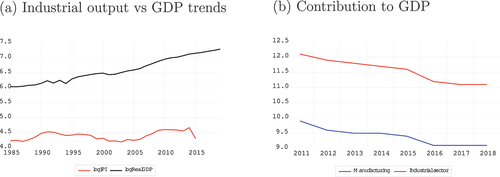
As of 2018, the industrial sector’s contribution to GDP stood at 11.1 percent (see 2019 Annual Economic Report). This added to a decade long downward trend of the sector’s contribution towards GDP, aided by the continuous decline in the share of manufacturing as can be seen in Figure 1(b).⁴ These trends reflect the fact that industrial activity has been growing at a slower pace compared to aggregate GDP. It is therefore the job of policy makers in Malawi to ensure that the trends in industrial production are reversed if structural transformation of the economy is to be achieved.

2.2. Malawi’s monetary policy in practice

The conduct of monetary policy in Malawi is guided by the Reserve Bank of Malawi Act of 1989 which was revised in 2018. The act mandates the RBM to formulate and execute monetary policy by using financial instruments at its disposal in to order to achieve stipulated economic objectives. Up until the revision of the Act in 2018, the stated objective of monetary policy had been “to implement measures designed to influence the money supply and the availability of credit, interest rates and exchange rates with the view to promoting economic growth, employment, stability in prices and a sustainable balance of payments position”.

In practice however, the bank has increasingly become more focused on stabilizing prices and less focused on the output and employment objectives. This is evident in its monetary policy statements which began to state that the main objective of monetary policy is to achieve low and stable prices, that preserve the value of the Kwacha, and encourages investment needed to achieve sustainable economic growth and employment creation”. Accordingly, the revised Act of 2018 recasts the objective of monetary policy which now states: “the primary objectives of the Bank is to maintain price and financial stability”. The revised Act further states: “in case of conflict between price and financial stability, the price stability objective shall take precedence”.

Operationally, the RBM has two intermediate targets namely market interest rates and money supply as measured by broad money (M2). In targeting money supply, the bank tracks the growth of the monetary base (M0) and does so using several instruments that include the bank’s policy rate (RBM bank rate), Open Market Operations (OMOs), Liquidity Reserve Requirement (LRR), and purchases and sales of foreign exchange. These instruments have direct links with both M0 and market interest rates. The bank rate for instance serves as a reference rate for commercial banks’ interest rates and OMOs, LRR and foreign exchange purchases/sales directly alters M0. Whether or not the two intermediate targets affect the bank’s principle objectives is an empirical matter.

In terms of the bank’s monetary policy stance, it can be argued that over the last couple of years the RBM pursued monetary policy characterized by notable inconsistencies. This is because the bank typically maintained high interest rates while at the same time growing the monetary base at a high rate. Between 2005 and 2019, the bank’s policy rate averaged 19.58 percent while the monetary base grew at an annual average of 26.2 percent, peaking at 51.5 percent in 2008. This shows that whilst the bank’s interest rate policy was contractionary, the rate at which it grew the monetary base was characteristic of an expansionary policy.

The RBM’s inconsistency on the stance of monetary policy suggests is that it likely uses the bank rate and reserve money for different policy objectives regardless of whether these objectives are in conflict with one another. Specifically, the policy rate appears to be mainly used for controlling inflation while reserve money is mainly used for moderating business cycles. This observation is empirically supported by Ngalawa and Viegi (2012) who showed that the RBM would respond to a drop in output by increasing the monetary base while at the same time raising the bank rate. The former is consistent with moderating the business cycle while the later suggests attempts at price stabilization.

3. Literature review

This section provides a review of monetary policy in theory and practice. In particular, the Classical, Keynesian and monetarists views of monetary policy transmission and effectiveness are compared before reviewing the empirical evidence for Malawi and other developing countries.

3.1. Monetary policy in theory: Effectiveness and transmission

3.1.1. The classical view

Classical economists believed that the economy is always in or near equilibrium such that changes in economic policy variables are fully absorbed by prices. As such, monetary policy that increases money supply would only lead to a rise in prices and not changes in real output. At the core of this view is the “equation of exchange” which is an identity that links money supply ($M$), money velocity ($V$), real output ($Y$), and prices ($P$). The equation given as

$MV=PY$

which states that nominal output ($PY$) or the money value of all goods and services supplied in the economy equals the total amount of money circulating in the economy times the number of times it circulates.

With the assumption that the economy is in equilibrium, classical economists treat $Y$ in the equation of exchange as fixed. Furthermore, $V$ is also assumed to be stable over time and therefore is fixed as well. Fixing $Y$ and $V$ in the equation at $\bar{Y}$ and $\bar{V}$ , respectively, we get

$M\bar{V}=P\bar{Y}$

This means that any increase in $M$ by the monetary authorities results in a proportional increase in $P$ and no changes in $Y$. This is the so called neutrality of money.

3.1.2. The Keynesian view

The Keynesian view of monetary policy rejects the classical economists’ idea that the economy is always at or near the equilibrium levels such that real output in the equation of exchange can be assumed to be fixed. The Keynesians school of thought posits that price and wage setting rigidities prevent immediate price and wage adjustments thereby creating periods of disequilibrium in the economy where monetary (and fiscal) policy can be used effectively to manipulate aggregate demand and by extension real output.

At the core of’ Keynesian models are three equations which govern the short-run dynamics between real output, investment, savings, employment, prices, and interest rates in the economy. These equations include the IS equation which shows levels of interest rates and output at which investment (I) equals saving (S), the Phillips equation depicting relationship between prices and real output or employment, and the Taylor rule which sets the short-term interest rates.

The Taylor rule sums up the Keynesian view of how monetary policy should be conducted in order to ensure stability of prices and output. The rule, as initially proposed by John B. Taylor,⁵ is given as

$i_t=r_t^{\ast }+1.5({\pi }_t-{\pi }_t^{\ast })+0.5(y_t-{\bar{y}}_t)$

where $i_t$ is the short-term nominal interest rate targeted by the central bank, $r_t^{\ast }$ is the equilibrium real interest rate, ${\pi }_t$ is the actual inflation rate, ${\pi }_t^{\ast }$ is the target inflation rate, $y_t$ is log of real GDP, and ${\bar{y}}_t$ is log of potential real GDP. Other versions of the Taylor rule have been proposed for different settings to include other variables deemed important by the particular central banks in question.

3.1.3. Monetarist View

The monetarist view which is mostly based on the work of Milton Friedman, sees money supply growth as the main determinant of short-run output and long-run inflation. This view sees money supply as an important factor determining aggregate demand in the economy which then translates into increased production. The idea behind is that consumers tend to maintain a certain level of money holdings and any significant deviation from this caused by increased money supply will result in increased consumption and investment expenditure as the consumers attempt to use up the excess money. This then creates the excess demand in the economy.

Central to the monetarist view is the Quantity Theory of Money (QTM) which is based on the equation of exchange. QTM treats $M$ in the equation of exchange as the main change inducing variable. $V$ on the other hand is taken to be relatively stable or predictable such that we have

$M\bar{V}=PY$

This implies that increasing $M$ must result in increased $P$ or $Y$ or both. Precisely, the monetarist view posits that in the long-run $P$, will fully adjust to changes in $M$ and therefore monetary policy will affect output only in the short run and prices in the long run (long-run neutrality of money).

Given its view of money, real output and inflation, monetarism advocates for central banks to maintain a stable growth of money instead of discretionary policy targeting interest rates. Economist Bennett T. McCallum proposed the so called McCallum rule to guide central banks in adjusting money supply (reserve money) to achieve the desired levels of inflation and real output. This rule, an alternative to the Taylor rule, is given as

${\dot{m}}_t={\dot{m}}_{t-1}+{\bar{v}}_{t-16}+1.5(\bar{\pi }+\bar{y})+0.5{\dot{Y}}_{t-1}$

where ${\dot{m}}_t$ is reserve money growth in quarter $t$, ${\bar{v}}_{t-16}$ is the average growth in the velocity of base money over the last 16 quarters, $\bar{\pi }$ is the inflation target, $\bar{y}$ is the long-run average quarterly real GDP growth, and ${\dot{Y}}_{t-1}$ is the nominal GDP growth for the quarter $t-1$.

3.2. Evidence of monetary policy effectiveness

Impact of monetary policy on real output has been studied extensively and the results have been mixed. Several studies have focused on Malawi including Chavula (2016) who investigates the impact of monetary policy on some key macroeconomic variables using a small macroeconometric model. The paper finds no evidence that Malawi’s monetary policy affects real output. This is so despite the study showing that an upward adjustment in the policy rate has a positive impact on lending rates and negative impacts on money supply. A lack of monetary policy effectiveness was also found by Mangani (2012) but with regard to prices. He too found that monetary policy implemented through a policy rate adjustment was capable of affecting lending rates and credit supply but this did not transmit to prices.

Other studies on Malawi’s monetary policy have given a more positive verdict regarding the effectiveness of monetary policy in stimulating growth. Like Mangani (2012), Ngalawa and Viegi (2012) used the VAR approach to analyze the dynamic effects of monetary policy in Malawi. In this study, shocks to the policy rate and reserve money (the two monetary policy operating targets for the RBM) were identified and analyzed with respect to their impact on aggregate output and prices and the transmission mechanisms involved. The study found that both the policy rate and reserve money did in fact affect real output by causing Malawi’s GDP to decline when the RBM raised the policy rate or reduce reserve money. The money effect and bank lending channels were established as the transmission mechanisms for that enabled these effects. The study found no link between monetary policy and exchange rates, but nevertheless the latter was found to be the most important factor in the determination of prices and an important variable for determining output.

A significant impact of monetary policy on real GDP was also found by Chiumia (2015) who used the Factor Augmented Vector Autoregressions (FAVAR) to eliminate the price and liquidity puzzles that are found in the other studies using ordinary VARs. This study found that positive interest rate shocks induced a negative reaction in GDP in line with Keynesian school of thought. No impact of base money innovations on real GDP was found although broad money showed a positive impact on GDP. The study also concludes that policy reversals in monetary and exchange rate policies could be responsible for the monetary policy ineffectiveness found in other studies.

In his work using a Time Varying Parameter VAR (TVP-VAR), Mwabutwa et al. (2016) found that prior to the year 2001, monetary policy transmission mechanisms were unclear and monetary policy had no impact on real output. However, after 2001, policy rate changes did affect GDP but in a rather non-conventional way whereby a rise in the RBM bank rate caused an increase in GDP. The study further found the interest rate channel and the exchange rate channel to be functional and in line with theory while the credit channel was found to be weak.

Aside from the VAR based literature, there has been other studies have used the general equilibrium framework to study monetary policy in Malawi. Matola and Gonzalez (2019) used a New Keynesian Dynamic Stochastic General Equilibrium (NK-DSGE) model to study monetary policy rules in Malawi. The study showed a functional and effective Taylor type of monetary policy rule whereby the central bank responded to inflation more strongly than to output. Nonetheless, positive adjustments to the policy rate were found to be effective in moderating real output in line with the postulations of the new Keynesian theory. Similary Bangara (2019) who also uses a NK-DSGE to investigate implications of foreign exchange constraints on key macroeconomic variables in Malawi, also finds that monetary policy was effective in influencing output.

Although no studies linking monetary policy to the industrial sector specifically have been done in Malawi, some literature on other developing countries exists. Ezeaku et al. (2018) in their study on the industry effects of monetary policy transmission channels in Nigeria found that there was a a long-run relationship between monetary policy and real output growth in the industrial sectors of Nigeria. The study used an ARDL model to show that private sector credit, interest rate, and exchange rate were functional transmission channels from monetary policy to Nigeria’s industrial output.

On their part, Kutu and Ngalawa (2016) looked at the impact of monetary policy on industrial output in South Africa using a structural VAR model fitted with monthly data from 1994 to 2012. The study finds a positive impact of money supply shocks on industrial output. However, interest rates and exchange rates are found to have no bearing on industrial growth. Overall, the study concludes that monetary authorities in South Africa had limited control over the country’s industrial sector. More definitive results are found by Pandey and Shettigar (2018) in the case of India. Their study used a Vector Error Correction Model (VECM), an ARDL—bounds test model, and VAR to estimate the short-run and long-run relationships between broad money and weighted average lending rate (WALR) on one hand and industrial production on the other hand. Their results show that both monetary variables affected India’s industrial output and that policy to control only inflation would adversely affect the country’s industrial sector.

4. Methodology

Four methodological approaches are employed for the econometric analysis carried out in this study. These include: the Autoregressive Distributed Lag (ARDL) model, Least Squares with Breakpoints model, Conditional Error Correction (CEC) model (bounds test), and the Vector Autoregression (VAR) model. The first two models are used for analyzing the overall responsiveness of industrial output to changes in monetary policy, the CEC model is used to isolate short-run effects from the long-run impact of monetary policy, and lastly the VAR model is used to analyze the short-run dynamics between industrial production and monetary policy and the transmission mechanisms involved. Sections 4.1–4.3 provide the theoretical backgrounds for the four models and section 4.4 describes the actual variables that are used in the models in this paper.

4.1. Autoregressive distributed lag models

The ARDL model is a single equation standard least squares regression model that includes lags of the dependent variable as regressors in addition to other explanatory variables and their lags. For a given regressand $y$, explanatory variables $x_i$, deterministic terms $w$, and parameters $\theta$, ${\beta }_i$, and $\gamma$, the ARDL model can be expressed as follows.

(1) $\theta (L,p)y_t=\sum _{i=1}^k{\beta }_i(L,q_i)x_{i,t}+\gamma w_t+{\epsilon }_t$(1)

where $L$ is the lag operator, and $\theta (L;p)\equiv 1-{\theta }_{1}L-{\theta }_2{L}^2-\dots -{\theta }_p{L}^p$ and $\beta (L,q_i)\equiv \hspace{0.17em}1-{\beta }_{i1}L-{\beta }_{i2}{L}^2-\dots -{\beta }_{i}q{L}^{q_i}$ are lag polynomials such that for a given variable $z_t$, $L^0{z}_t\equiv z_t$, $L^1{z}_t\equiv z_{t-1}$, $L^2{z}_t\equiv z_{t-2}$, and so on and so forth. ${\epsilon }_t$ is a residual term.

The ARDL model can be cast in several different representations depending on the kind of relationships between the variables that one wants to observe. The conditional error correction form is arguably the most interesting representation of the model, in part due to its ability to capture both the short-run and long-run effects of the explanatory variables on the explained variable. The method, known as the ARDL cointegration technique or bound cointegration technique, involves first testing for cointegration using the bounds test and then fitting the error correction form of the model.

The ARDL cointegration technique has become a popular analytical tool for single equation time series analysis following the works of H. M. Pesaran and Shin (1999) and H. M. Pesaran et al. (2001). The technique has the advantage that it can be used to analyze cointegrating relationships without necessitating prior determination of the order of integration of the variables in the model. Thus one can apply this method to a set of data that contains I(0) variables, I(1) variables, or a mix of both.

The ARDL cointegration model can be derived by applying some mathematical manipulations to equation (1)(1) $\theta (L,p)y_t=\sum _{i=1}^k{\beta }_i(L,q_i)x_{i,t}+\gamma w_t+{\epsilon }_t$(1) in order to get

(2) $\mathrm{\Delta }{y}_t=\gamma w_t+\theta (1)E{C}_{t-1}+({\tilde{\theta }}^{\ast }(L)\mathrm{\Delta }{y}_{t-1}+\sum _{i=1}^k{\tilde{\beta }}_i(L)\mathrm{\Delta }{x}_{i,t-1})+\sum _{i=1}^k{\beta }_i(L)\mathrm{\Delta }{x}_{i,t}+{\epsilon }_t$(2)

where ${\tilde{\theta }}^{\ast }(L)\equiv (1-L{)}^{-1}({\theta }^{\ast }(L)L^{-1}-\theta (1))$ for ${\theta }^{\ast }(L)\equiv {\sum }_j^p{\theta }_j{L}_j$ and ${\tilde{\beta }}_i(L)\equiv (1-L{)}^{-1}({\beta }_i(L)-{\beta }_i(1))$, and $E{C}_t\equiv y_t-{\sum }_{i=1}^k{\beta }_i(1)x_{i,t}$ is the error correction term when $y_t$ and $x_t$ are cointegrated.

4.2. Least squares with breakpoints

To incorporate potential structural breaks in the data, an analysis using the Least Squares with Breakpoints technique (hereinafter LSBP) is also conducted. The LSBP method is useful for situations where some variables in the model are known to have changed structurally and the exact periods in which the structural change occurred are known before hand. Estimating the model therefore requires that the breaking variables and the breakpoints are identified first before estimation is done. This can be done with the aid of apriori information or econometric based techniques such as the sequential breaks test. The model is estimated as follows.

Let $X_t$ be a set of variables that do not have any structural breaks over the sample period, and $Z_t$ be the set of variables that have $m\ge 1$ breaks corresponding to $r=m+1$ regimes in the sample period. The regression equation may be specified as

(3) $y_t=X_t\zeta +Z_t{\delta }_r+{\mu }_t$(3)

where $\zeta$ is the set of time invariant coefficients for the non-breaking regressors, ${\delta }_r$ are the regime specific parameters for the breaking regressors, and ${\mu }_t$ is the residual term. The LSBP method estimates equation 3(3) $y_t=X_t\zeta +Z_t{\delta }_r+{\mu }_t$(3) by introducing regime dummy variables to get

(4) $y_t=X_t\zeta +{\tilde{Z}}_t\tilde{\delta }+{\tilde{\mu }}_t$(4)

where ${\tilde{Z}}_t$ is an expanded set of regressors derived by interacting $Z_t$ with the regime dummies, and $\tilde{\delta }\equiv ({\delta }_1,\dots ,{\delta }_r)$ are the estimated regime specific parameters. Equation 4(4) $y_t=X_t\zeta +{\tilde{Z}}_t\tilde{\delta }+{\tilde{\mu }}_t$(4) is then estimated using standard regression techniques.

4.3. Vector autoregression model

For the analysis of the short-run dynamics and transmission mechanisms from monetary policy to industrial production, the study makes use of the VAR approach. VAR models are simple yet very useful tools for analyzing interrelationships between variables that potentially have feedback effects among each other. The model is expressed as a system of equations in which each variable in the system is dependent on its own lags and the lags of all the other variables.

In the VAR literature, an important distinction is made between a reduced form VAR and a structural VAR. Reduced form VARs are estimated without imposing any theoretically based restrictions and as such one can not draw causal inferences between the variables, but rather only how they move together. Though adequate for forecasting, one can not use reduced form VARs to establish how changes in one variable affects the other variables. Doing so requires transforming the reduced form VAR into a structural VAR by imposing theory based restrictions so that structural shocks can be identified and causal effects observed. To see how structural VARs and reduced form VARs relate to one other, consider the following.

Let $X_t$ denote the column vector of $n$ endogenous variables forming a system of dynamic equations. Further, let the structural VAR(p) model for $X_t$ with lags $j=1,2,\dots ,p$ take the form

(5) $X_t=\alpha +A_0{X}_t+\sum _{j=1}^p{A}_j{X}_{t-j}+u_t$(5)

where $\alpha$ is the $n\times 1$ vector of intercepts, $A_0$ and $A_j$ are $n\times n$ matrices of structural coefficients, and $u_t$ is an $n\times 1$ vector of orthogonal disturbances with zero mean and variance, ${\sum }_u=I_n$. Note that equation (5)(5) $X_t=\alpha +A_0{X}_t+\sum _{j=1}^p{A}_j{X}_{t-j}+u_t$(5) can not be estimated due to the presence of the dependent variables on the right hand side of the equation. However, it can be transformed into its estimable reduced form counterpart by solving for $X_t$ and deriving the reduced form coefficients to get

(6) $X_t=\beta +\sum _{j=1}^p{B}_j{X}_{t-j}+e_t$(6)

where $\beta \equiv (I_n-A_0{)}^{-1}\alpha$ and $B_j\equiv (I_n-A_0{)}^{-1}{A}_j$ are the coefficients of the reduced form model, and $e_t\equiv (I_n-A_0{)}^{-1}{u}_t$ is a vector of correlated forecast errors with zero mean and variance, ${\sum }_e$.

The task therefore is to identify the matrix ($I_n-A_0$), which enables us to derive equation (5)(5) $X_t=\alpha +A_0{X}_t+\sum _{j=1}^p{A}_j{X}_{t-j}+u_t$(5) from equation (6)(6) $X_t=\beta +\sum _{j=1}^p{B}_j{X}_{t-j}+e_t$(6) . A number of identification strategies have been proposed and used in literature one of which is the recursive ordering method. In a recursive VAR, variables are ordered according to their level of exogeinity within the system and the matrix ($I_n-A_0$) is set to be the inverse of the Cholesky factor of ${\sum }_e$. Therefore, the structural model is identified based on the presumed contemporaneous relationships between the variables. In our case, it is assumed that the policy variables affect the policy objectives contemporaneously while the objective variables affect policy with a time lag. This follows the argument by Stock and Watson (1989) and Bernanke and Blinder (1992) who argue that delays in the availability of economic data make policy makers to also delay policy implementation.

Whilst the recursive ordering method is easy to implement, it suffers the drawback that the results tend to be sensitive to the ordering of the variables thus making identification of shocks not so robust. To address this problem, H. Pesaran and Shin (1998) proposed the generalized impulse analysis which does not require orthogonalization of shocks and does not depend on the ordering of the variables in the VAR. In this study, this approach is used in the derivation of the impulse responses and variance decomposition analysis.

4.4. Data and sources

The study uses monthly data spanning a period of 146 months from 2004/04 to 2016/05.⁶ For the two ARDL models, the LSBP model, and the baseline VAR model, 5 variables are used and these include: industrial production ($ip$), inflation rate ($inf$), exchange rate ($ex$), monetary base ($mb$), and the policy rate ($br$). Additional variables including the lending rate ($lr$), bank loans to the private sector ($bl$), broad money ($m2$), and consumer price ($cp$) are used in the analysis of monetary policy transmission mechanisms.

Actual definitions of the data series used for each variable and the sources are given in Table 1. $ip$ is the IMF’s industrial production index (base year = 2010). $inf$ is the IMF’s monthly inflation rate defined as percentage change in consumer prices ($cp$) measured by the Consumer Price Index (CPI). The two interest rates, $br$ and $lr$, are nominal rates provided by the RBM. The rest of the series ($mb$, $m2$, $ex$, and $bl$) are level form nominal values also sourced from the RBM and these, together with $ip$ and $cp$, are transformed into their natural logarithms. All variables are tested for stationarity using the Augmented Dickey Fuller unit root test and the results are also indicated in Table 1.

Table 1. Data description and sources

Variable	Series Used and Order of Integration	Source
industrial output, $ip$	industrial production index (base = 2010) - I(0)	IFS
consumer price, $cp$	consumer price index (base = 2010) - I(1)	IFS
inflation, $inf$	percentage change in CPI - I(0)	IFS
exchange rate, $ex$	Malawi Kwacha per US dollar exchange rate - I(1)	RMB
monetary base, $mb$	monetary base - I(1)	RMB
policy rate, $br$	RBM bank rate - I(1)	RMB
lending rate, $lr$	commercial banks’ average lending rate - I(1)	RMB
bank loans, $bl$	banking systems’ gross claims on private sector - I(1)	RMB
money supply, $m2$	broad money (m2) - I(1)	RMB

5. Results and analysis

In this section, estimation results from the econometric models described in section 2 are presented. For the ARDL models and the LSBP model, the elasticities of industrial output ($ip$) due to changes in monetary policy ($br$ and $mb$) are analyzed for each of the models. For the VAR model, the results are presented in the form of impulse responses and forecast error variance decomposition (FEVD). The former shows the short-run dynamic effects of identified shocks while the latter indicates percentage contribution of each shock to the variations in the variables in the model. The main findings can be summarized as follows.

1. Tight monetary policy has a negative impact on industrial production both in the short run and in the long run.

2. Market interest rates and money supply are the main transmission channels through which this effect takes place.

3. Aside from own shocks, variations in industrial output are mainly due to changes in monetary policy.

5.1. Trend analysis

Before analyzing the causal relationships between monetary policy and industrial production, a trend analysis of the variables is conducted so as to show how monetary policy and industrial output have associated with one another overtime. Therefore, trends in industrial activity are compared with those of the RBM bank rate and money supply.

Panel (a) of Figure 2 plots the annual growth rate of industrial output (IP_GROWTH) against the annual average of the bank rate (BR) while panel (b) plots the log of industrial production (LOG_IP) against the log of base money (LOG_MB). The graphs show that between 2005 and 2015, growth of industrial output and the bank rate moved in opposite directions while industrial output and money supply both trended upwards albeit at different paces. Correlation analysis show that the bank rate and industrial production growth (IPGR) have a Pearson correlation coefficient of −0.49 while that of base money and industrial output is 0.48. These trends would be consistent with a negative (positive) reaction of industrial production following tightened (loosened) monetary policy, an issue explored in more detail in sections 5.2 and 5.3 below.

Figure 2. Industrial production and monetary policy trends.

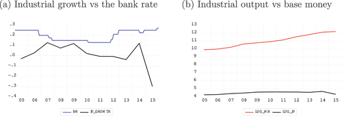
Figure 2 further shows that while the RBM maintains high interest rates, it simultaneously grows the monetary base at a high rate. This observation is confirmed in Table 2 where it is shown that between 2005 and 2015, the bank rate averaged 19.7 percent and at its lowest point it only fell to 13 percent. Money growth on the other hand averaged 26.2, reaching a maximum growth rate of 51.51 percent in 2008. This shows that the monetary authorities have been inconsistent on the stance of monetary policy and this has the potential to slow economic activity including that of the industrial sector whose annual growth over that same period averaged only 1.13 percent.

Table 2. Descriptive statistics for monetary policy and industrial production

	bank rate	base money growth	industrial output growth
Mean	19.74	26.22	1.13
Median	18.54	24.63	12.79
Maximum	25.33	51.51	2016
Minimum	13.00	7.45	−29.62
Std.Dev	5.02	14.76	11.89

5.2. Short-run impact of monetary policy on industrial output

The analysis of the impact of monetary policy on industrial output in the short run is based on the ARDL and LSBP models. The CEC model in section 4.3 looks at both short-run and long-run impacts. The number of lags to be included for each variable in the ARDL models is determined by the Hannan-Quinn criterion which suggests 4 lags for $ip$, 2 lags for $br$, and no lags (only contemporaneous effects) for $mb$, $ex$, and $inf$. Same lag structure is maintained in estimating the LSBP model. As for the structural breaks in the LSBP model, these are determined by the Bai-Perron test which finds one structural break at 2013/12. Results of the two models are presented in Table 3.

Table 3. ARDL and LSBP parameter estimates

	ARDL	LSBP
Dep. var : $i{p}_t$		2004/04–2013/12	2014/01–2016/5
$b{r}_t$	0.36 (0.99)	−0.30 (0.96)
$b{r}_{t-1}$	−3.49 (1.25)**	−3.63 (1.20)
$b{r}_{t-2}$	2.42 (0.89)**	3.00 (0.87)**
$m{b}_t$	0.16 (0.05)**	0.18 (0.06)**
$e{x}_t$	0.17 (0.08)*	−0.11 (0.10)
$in{f}_t$	0.00 (0.01)	0.01 (0.01)
$i{p}_{t-1}$	0.79 (0.08)**	0.67 (0.07)**
$i{p}_{t-2}$	−0.12 (0.10)	−0.12 (0.10)
$i{p}_{t-3}$	0.01 (0.10)	0.01 (0.10)
$i{p}_{t-4}$	−0.23 (0.07)**	−0.30 (0.07)**
$cons.$	1.73 (0.32)**	2.05 (0.54)**

Notes: Values in the parentheses are standard errors. ** and * mean coefficient is significant at 1% and 5%, respectively.

Although the two models both show no evidence contemporaneous impact of $br$ on $ip$, lagged effects were found in both models. Specifically, the ARDL model estimates that a 1 percentage point increase in $br$ in month $t$ caused $ip$ to decrease by 3.49 percent in month $t+1$. However, in month $t+2$, $ip$ gained 2.42 percent of the initial amount. Similar results are found with the LSBP model which estimates that during the first regime (2004/04–2013/12), $ip$ decreased by 3.63 percent in month $t+1$ following a 1 percentage point rise in $br$ in month $t$, but gained 3.0 percent in month $t+2$. The impact of $br$ was much greater in regime 2 (2014/01–2016/05) where a 1 percentage point increase in $br$ caused $ip$ to decline by 8.08 percent after two months.

For changes in money supply, the two models also give similar results as both show that expanding the monetary base leads to higher industrial output. Specifically, increasing $mb$ by 1 percent caused $ip$ to rise by 0.16 percent per the ARDL model, and by 0.18 percent and 0.23 percent in the first and second regimes of the LSBP model, respectively. These findings support the theoretical expectation that tight (loose) monetary policy negatively (positively) affects industrial output.

In terms of inflation and exchange rate shocks, the ARDL model finds significant evidence that the exchange rate affects industrial output but no evidence for inflation effects. The parameter estimate for $ex$ shows that a 1 percent depreciation of the domestic currency causes industrial output to decline by 0.17 percent. This can be explained by the fact that Malawi is a net importer which relies heavily on imported inputs for production, thus a depreciation of the Malawi Kwacha increases the cost of production in the sector thereby reducing its output. However, contrary to the ARDL model, results of the LSBP model show no evidence on the impact of the exchange rate and some significant impact of inflation. In the second regime, inflation is shown to have a negative impact on industrial the sector which declines by 0.04 percent following a 1 percentage point rise in inflation.

5.3. Long-run impacts of monetary policy on industrial output

In order to isolate the long-run impact of monetary policy from the short-run effects, a CEC model is estimated and the PSS (2001) bounds test conducted. The results, which are presented in Table 4, show the existence of a long-run relationship between monetary policy and industrial production. This finding is confirmed by both the long-run parameter estimates and the bounds test in Table 5 where the null hypothesis that there is no cointegration is rejected at 1 percent significance level. The estimated parameters show that a 1 percentage point increase in the RBM bank rate causes industrial output to decline by 1.26 percent in the long run. Furthermore, when the monetary base is increased by 1 percent, it results in a 0.29 percent increase in industrial production. The speed of adjustment to the long-run equilibrium, the error correction term, is found to be 0.55.

Table 4. ARDL conditional error correction model

Dep. Var: $\mathit{i}{p}_t$
		Coeff.	Std. Err
Long run
	$ECT$	−0.55**	0.07
	$b{r}_{t-1}$	−1.26*	0.63
	$m{b}_{t-1}$	0.29**	0.09
	$e{x}_{t-1}$	−0.31*	0.14
	$in{f}_{t-1}$	−0.00	0.02
	cons.	3.16**	0.39
Short run
	$\mathrm{\Delta }i{p}_{t-1}$	0.34**	0.07
	$\mathrm{\Delta }i{p}_{t-4}$	0.22**	0.07
	$\mathrm{\Delta }i{p}_{t-3}$	0.23**	0.07
	$\mathrm{\Delta }b{r}_{t-1}$	0.37	0.85
	$\mathrm{\Delta }b{r}_{t-2}$	−2.43**	0.85

Note: ** and * imply significance at 1% and 5%, respectively.

Table 5. H. M. Pesaran et al. (2001) F-Bounds test

${\mathit{H}}_o$: no level relationship							$\mathit{F}=9.827431$
	Kripfganz and Schneider (2018) critical values
	$\mathbf{10}\mathbf{\%}$		$\mathbf{5}\mathbf{\%}$		$\mathbf{2.5}\mathbf{\%}$		$\mathbf{1}\mathbf{\%}$
	I(0)	I(1)	I(0)	I(1)	I(0)	I(1)	I(0)	I(1)
$F$	2.2	3.09	2.56	3.49	2.88	3.87	3.29	4.37

The CEC model also estimates the short-run effects of monetary policy and the results agree with those of the ARDL and LSBP models shown above. Looking at the estimated coefficients of $\mathrm{\Delta }b{r}_t$, we see that there is no contemporaneous impact of the policy rate on industrial production. The impact is lagged one period where a 1 percentage point increase in $br$ in period $t$ causes a 2.42 percent drop in industrial output in period $t+1$. These results also confirm the expectation that tight monetary policy reduces output and loose monetary policy boosts production.

The findings from all the three models above regarding the impact of monetary policy are consistent with the findings of Chiumia (2015) and Ngalawa and Viegi (2012) both of whom worked within the VAR framework and showed that monetary policy in Malawi affected real aggregate output as per the predictions of macroeconomic theory. Similar results were also found by Matola and Gonzalez (2019), and Mwabutwa et al. (2016) whose studies employed estimated DSGE models. Furthermore, these results are also comparable to what Pandey and Shettigar (2018) and Ezeaku et al. (2018) found in the cases of India and Nigeria respectively. Both studies showed that tight monetary policy negatively affected production the industrial sector. As a result of their findings, Pandey and Shettigar (2018) recommended that monetary policy in India should not be overly focused on controlling inflation but rather it should also be mindful of the implications that it has on industrial activity. The same recommendation is made in this study.

5.4. Dynamic effects of monetary policy on industrial output

In order to understand the dynamic effects of monetary policy, a structural VAR model is estimated as per procedure explained in section 4.3. The model is fitted with all five variables ($br$, $mb$, $ex$, $inf$, and $ip$) in levels even though $br$, $mb$ and $ex$ are found to be non-stationary. This practice has become common in VAR literature since the work of Sims (1980) who showed that estimates derived in such a way are still consistent. For the lag order, all the econometric based lag selection criteria recommend lag structures whose models are not stable as the highest root of the characteristic polynomial lie outside the unit circle (see Table A1 for lag recommendations). In fact, among all models with lags between 1 and 6, only VAR (2) models are found to be stable (Table A2). For this reason I proceed to estimate the VAR (2) models.

5.4.1. Impulse response analysis

For a shock increase in the bank rate, the single period and accumulated impulse responses of industrial production are depicted in panels (a) and (b) of Figure 3. There it is shown that a positive shock to the bank rate induces a decline in industrial output within three months following the shock. This decline is quite persistent as it goes beyond 18 months without rebounding to the pre-shock levels. Furthermore the accumulated impulse response show that cumulatively the overall impact of the bank rate shock remains negative which further confirms the results from the ARDL, LSBP, and CEC models.

Figure 3. Impulse response of industrial production to monetary policy shocks.

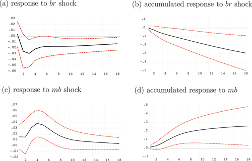
With regard to the impact of a money supply shock, panels (c) and (d) of Figure 3 show the single period and accumulated impulse responses of industrial production given a shock to the monetary base. There it is shown that a monetary expansion through an increase in the monetary base results in increased industrial output. This effect also takes place within three months of the shock and lasts at least another four months. As for the overall impact as suggested by the accumulated impulse response, the VAR results are also indicate a positive impact of monetary policy on industrial output, a result that is also consistent with the findings from the ARDL, LSBP, and CEC models.

As a check to these findings, the Granger Causality tests is carried out in order to confirm the causal direction between the monetary policy variables and industrial output. Results of the test are presented in Table 6. There it is shown that whilst we can not conclusively determine the causal direction between money supply and industrial output using this test, we can conclusively say that changes in the policy rate indeed affect industrial production. Interestingly though, shocks to industrial production do not induce changes in monetary policy which suggests that the monetary authorities in Malawi do not react to cycles in the industrial sector. This is perhaps due to the fact that monetary policy is focused on other objectives such low inflation and stable exchange rate as Table 6 further suggests.

Table 6. Pairwise granger causality test

Null Hypothesis	F-statistic	p-value
$br$ does not Granger cause $ip$	9.43587	0.0001
$ip$ does not Granger cause $br$	0.31229	0.7323
$mb$ does not Granger cause $ip$	1.36623	0.2584
$ip$ does not Granger cause $mb$	0.18395	0.8322
$cp$ does not Granger cause $br$	6.67746	0.0017
$ex$ does not Granger cause $br$	5.88303	0.0035

5.4.2. Variance decomposition analysis

In order to determine how much influence monetary policy has on industrial production relative to the other shocks in the model, the forecast error variance decomposition for industrial production is analyzed. The results are reported in Table 7 where it is shown that aside from own shocks, policy rate and money supply shocks are the most important determinants of industrial production. Overtime, up to 12.4 percent of the variation in industrial production is attributable to movements in the policy rate and 11.7 percent can be attributed to money supply shocks. This implies that changes in monetary policy are responsible for about 24 percent of the movements in industrial production. The exchange rate and inflation account for 7.2 percent and 5.6 percent respectively. These results also support the findings from the ARDL models in that they confirm the long-run relationship between monetary policy and industrial production.

Table 7. Forecast error variance decomposition for industrial production

Month	br	mb	ex	cp	ip
1	0.13	1.73	0.00	0.02	98.10
3	3.74	4.05	0.45	2.54	89.19
6	5.43	11.12	5.81	5.29	72.33
9	6.96	12.17	6.85	5.30	68.70
12	8.38	12.23	6.89	5.32	67.16
18	10.33	12.11	6.94	5.44	65.15
24	11.43	11.95	7.03	5.54	64.03
30	12.05	11.82	7.13	5.61	63.36
36	12.40	11.76	7.25	5.65	62.91

5.5. Transmission mechanisms from monetary policy to industrial production

Having established the impact that monetary policy in Malawi has on the county’s industrial output, the actual transmission mechanisms at play are examined next. Three monetary policy transmission mechanisms that are deemed relevant to Malawi are investigated and these include: the interest rate channel, the money supply channel, and the exchange rate channel. Each of these channels is investigated using a different specification of the VAR model such that the only variables included are those involved in the transmission, in addition to industrial production and prices. This is done to avoid using one over-parameterized model and also to minimize possible multicollinearity. This approach is used also in other previous studies including Ngalawa and Viegi (2012) and Mangani (2012).

5.5.1. Interest rate channel

The interest rate channel posits that monetary policy affects real output and prices via its effect on market rates and therefore on the cost of credit. Tight monetary policy for instance causes both nominal and real market interest rates to rise and this is enabled by the rigidity of prices. The rise in real interest rates translates into increased cost of borrowing and this causes households and firms to cut back on investment thus leading to a decrease in output.

For countries whose financial sectors are dominated by commercial banks, the interest rate channel is one of the more relevant transmission channels given that in such circumstances the banking system plays the biggest role in transmitting monetary policy. In the case of Malawi, bank lending happens to be the main source of external financing for firms as evidenced by the low participation of firms on the local capital market. This renders the interest rate channel potentially an important monetary policy transmission channel in Malawi.

To investigate this channel, a VAR model containing the monetary policy variables, commercial banks’ lending rate, commercial bank’s loans to the private sector, and the monetary policy objective variables is estimated. Thus from equation 2(2) $\mathrm{\Delta }{y}_t=\gamma w_t+\theta (1)E{C}_{t-1}+({\tilde{\theta }}^{\ast }(L)\mathrm{\Delta }{y}_{t-1}+\sum _{i=1}^k{\tilde{\beta }}_i(L)\mathrm{\Delta }{x}_{i,t-1})+\sum _{i=1}^k{\beta }_i(L)\mathrm{\Delta }{x}_{i,t}+{\epsilon }_t$(2) , the vector of endogenous variables $X_t$ is set as:

$X_t=[brmblrblcpip{]}^T$

where $lr$ is commercial banks’ lending rate, $bl$ is amount of bank loans extended to the private sector, and $br$, $mb$, $cp$ and $ip$ are as defined before.

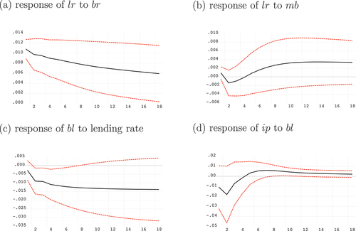
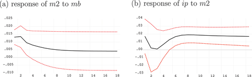
The impulse responses depicting the transition mechanism are presented in Figure 4. There it is shown that lending rates are influenced by shocks to the policy rate but not by shocks to the monetary base. Specifically, an increase in the policy rate results in an immediate and persistent rise in lending rates (Figure 4a). This is because in Malawi the policy rate acts as the reference rate for commercial bank rates. The rise in the lending rates results in lower private sector borrowing (Figure 4c). Finally, the impact of decreased borrowing on industrial production is shown in Figure 4d where a positive relationship between bank loans and industrial production is established. There it is shown that higher (lower) credit today causes industrial output to rise (decline) within 8 months. Put together, these results offer evidence that adjusting the policy rate can affect industrial output through the interest rate channel.

Figure 4. Impulse responses for the interest rate channel.

5.5.2. Money supply channel

The money supply channel is derived from the quantity theory of money which emphasizes the importance of money supply in influencing real output. The idea is that a sudden increase in the quantity of money will lead to higher spending by economic agents due to the perceived increase in real income. This perception is a result of failure by the economic agents to correctly interpret the increase in their money holdings as inflationary. The increased spending results in increased output by producers.

To capture the money supply channel, a model is estimated in which broad money is included to measure money supply in the economy. Furthermore, the policy rate is removed from the model and inflation rate replaced with aggregate prices, $cp$, to be more consistent with the specification of the quantity theory. Thus $X_t$, the vector of endogeneous variables for this model is set as:

$X_t=[mbm2cpip{]}^T$

where all variables are as defined before. The impulse responses are shown in Figure 5 where it is shown that a positive shock to the monetary base immediately increases broad money which in turn increases industrial production. The increase in industrial output is quite pronounced and persistent which indicates that money supply channel is one of the most effective monetary policy transmission mechanisms in Malawi at least in as far as industrial activity is concerned.

Figure 5. Impulse responses for the money supply channel.

5.5.3. Exchange rate channel

Last, the exchange rate channel for monetary policy transmission is investigated. For this channel, monetary policy works by altering the exchange rate which in turn affects competitiveness of internationally traded goods. On one hand, a depreciation of the domestic currency causes domestically produced goods to become relatively cheaper thereby enabling local firms to produce and export more. On the other hand, imported goods become relatively expensive which raises production costs for products that use imported inputs thereby putting negative pressure on their output.

With regard to how monetary policy can affect the exchange rate to begin with, there are two main ways. First, monetary policy affects market interest rates and therefore capital flows. A rise in market rates caused by tightening of monetary policy will attract capital in flows which would result in a strengthened domestic currency. Secondly, monetary policy can affect the exchange rate through changes in money supply. An increase in money supply for instance implies that there is more of the local currency to exchange with foreign currencies. The excess supply of the domestic currency would weaken it. In order to explore these mechanisms, the following model is estimated.

$X_t=[brmblrm2exinfip{]}^T$

Figure 6 presents selected impulse responses from this model. As the figure shows, no significant relationship is found between the exchange rate and market interest rates. However, an increase in broad money is associated with a depreciation of the domestic currency. Figure 6 further shows that a positive shock to the exchange rate (depreciation) leads to decreased industrial production. Although this is contrary to conventional thought, it is explainable by the fact that Malawi is a net importer which heavily relies on imported inputs for production activities. As such a depreciation of the domestic currency increases the cost of production which in turn causes a large enough decline in industrial output that offsets any export led gains in production.

Figure 6. Impulse responses for the exchange rate channel.

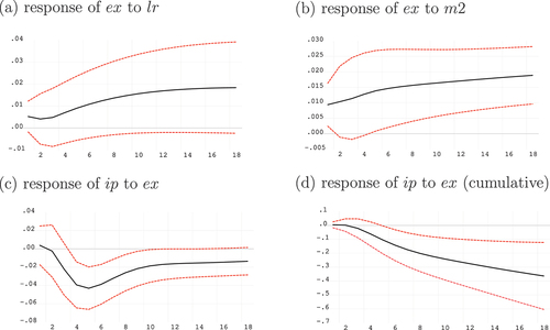
Since monetary authorities can affect broad money by altering the monetary base (recall from the discussion on the money supply transmission channel), they can therefore also affect industrial output through exchange rates. However, in this case it is a stronger domestic currency that benefits industrial production thus causing the exchange rate channel to work in opposite direction to the interest rate and money supply channels. Therefore, one can conclude that the exchange rate channel is not responsible for the negative impact of monetary policy on industrial production established in this study.

6. Conclusion and policy recommendations

In this paper, the impact of monetary policy on industrial production in Malawi is examined using ARDL and VAR models. The study finds that monetary policy affects industrial production regardless of whether the policy rate or the monetary base is used as the policy tool. Specifically, tight monetary policy lowers industrial output both in the short run and in the long run. The study also reveal that the interest rate channel and the money supply channel are two of the mechanisms that monetary policy is conventionally transmitted to industrial production. The exchange rate is another working transmission channel even though the transmission process deviates from the convention.

In view of these findings, the study recommends that the RBM should refrain from prolonged use of tight monetary policy in their quest to achieve stability of prices and the exchange rate. This contributes to the stagnation of the industrial sector. Rather monetary policy should be used only as a temporary measure to counter temporary shocks that threaten the attainment of the bank’s objectives. The country’s high inflation and depreciation rates should be considered structural issues that require structural changes.

Disclosure statement

No potential conflict of interest was reported by the author.

Additional information

Notes on contributors

Joseph Upile Matola

Joseph Upile Matola is an experienced economist who has worked as Principal Economist for Ministry of Economic Planning and Development in Malawi, specializing in macroeconomic policy analysis. He holds a Ph.D. in Development Economics from the National Graduate Institute for Policy Studies in Japan where he researched on various aspects of Malawi’s fiscal and monetary policies. He has also worked with the South African Institute of International Affairs where he has analyzed the macroeconomic impact of COVID-19 on 6 low- and middle-income countries in Africa.

Notes

1. The industrial sector is one of the areas prioritized in the Malawi Growth and Development Strategy.

2. Medina et al. (2017) estimates the that the informal sector contributes between 20 percent and 40 percent of Malawi’s GDP. Furthermore, according to the 2013 Malawi Labour Force Survey report, up to 89 percent of employed people in Malawi worked in the informal sector.

3. Per IMF’s definition, the industrial sector aggregates three activities from the International Standard Industrial Classification of All Economic Activities (ISIC) namely: manufacturing, mining and quarrying, and electricity and water supply.

4. See the Annual Economic Reports for 2019 and years before for sectoral shares of GDP and other national accounts information.

5. John B. Taylor was an economic adviser to US president George H. W. Bush. He proposed the rule in 1992 for the US Federal Reserve Bank to use in setting interest rates to stabilize prices and output.

6. The sample period reflects data availability particularly for industrial production index. Currently, Malawi’s industrial production index data in the IFS is updated with a 4 year time lag. At the time of the analysis the data was available only up to 2016/07. The last two observations are not included in our analysis because they cause instability of the VAR models. Nevertheless, including them does not affect the estimation results in terms of size and significance of parameter estimates.

Appendices

Table A1. VAR Lag Order Selection Criteria for the baseline model

Lag	LogL	LR	FPE	AIC	SC	HQ
0	−22.80307	NA	1.01e-06	0.380864	0.483042	0.422381
1	745.2263	1472.933	3.83e-11	−9.797620	−9.184551*	−9.548516*
2	780.1543	64.59283	3.34e-11	−9.933620	−8.809659	−9.476929
3	807.5899	48.85801	3.24e-11	−9.966985	−8.332132	−9.302707
4	831.9809	41.76536	3.29e-11	−9.958642	−7.812898	−9.086777
5	852.8053	34.23185	3.51e-11	−9.901442	−7.244806	−8.821990
6	873.5167	32.62753	3.78e-11	−9.842694	−6.675166	−8.555655
7	898.6482	37.86940	3.84e-11	−9.844495	−6.166076	−8.349870
8	925.6446	38.83054	3.84e-11	−9.871844	−5.682534	−8.169631
9	959.1425	45.88743	3.53e-11	−9.988253	−5.288051	−8.078453
10	990.4904	40.79527	3.38e-11	−10.07521	−4.864117	−7.957824
11	1027.947	46.17937	3.00e-11	−10.24585	−4.523864	−7.920876
12	1089.629	71.82160*	1.94e-11*	−10.74834*	−4.515467	−8.215783

* indicates lag order selected by the criterion

LR: sequential modified LR test statistic (each test at 5% level)

FPE: Final prediction error

AIC: Akaike information criterion

SC: Schwarz information criterion

HQ: Hannan-Quinn information criterion

Table A2. Roots of Characteristic Polynomial for baseline VAR (2) model

Root	Modulus
0.998642	0.998642
0.951352	0.951352
0.811676	0.811676
0.561987–0.264018i	0.620914
0.561987 + 0.264018i	0.620914
−0.328452	0.328452
0.051395–0.251406i	0.256605
0.051395 + 0.251406i	0.256605
0.233694	0.233694
−0.130116	0.130116

No root lies outside the unit circle.

VAR satisfies the stability condition.

References

- Bangara, B. C. (2019). A new Keynesian dsge model for low income economies with foreign exchange constraints. ERSA working papers (795).
- Bernanke, B. S., & Blinder, A. S. (1992). The federal funds rate and the channels of monetary transmission. The American Economic Review, 82(4), 901–21.
- Chavula, H. K. (2016). Monetary policy effects and output growth in Malawi: Using a small macroeconometric model. Open Journal of Modelling and Simulation, 4(4), 169–191. https://doi.org/10.4236/ojmsi.2016.44013
- Chiumia, A. (2015). Effectiveness of monetary policy in Malawi: Evidence from a factor augmented vector autoregressive model (favar). Macroeconomic, Finance Management Institute of Eastern, and Southern Africa.
- Ezeaku, H. C., Ibe, I. G., Ugwuanyi, U. B., Modebe, N., & Agbaeze, E. K. (2018). Monetary policy transmission and industrial sector growth: Empirical evidence from Nigeria. Sage Journals, 8(2), 215824401876936. https://doi.org/10.1177/2158244018769369
- Kripfganz, S., Schneider, D.C. 2018 ardl: Estimating Autoregressive Distributed Lag and EquilibriumCorrection Models 2018 London Stata Conference London 6-7 September
- Kutu, A. A., & Ngalawa, H. (2016). Monetary policy shocks and industrial sector performance in south Africa. Journal of Economics and Behavioral Studies, 8(3), 26–40. https://doi.org/10.22610/jebs.v8i3(J).1286
- Mangani, R. (2012). The effects of monetary policy on prices in Malawi. AERC Research Papers (252).
- Matola, J. U., & Gonzalez, R. L. (2019). Fiscal and monetary policy rules in Malawi: A new Keynesian dsge analysis. Grips Discussion Paper 19–03.
- Medina, L., Jonelis, A., & Cangul, M. (2017). The informal economy in sub-saharan Africa: Size and determinants. IMF Working Papers, 2017(156), 1. https://doi.org/10.5089/9781484305942.001
- Mwabutwa, C., Viegi, N., & Bittencourt, M. (2016). Evolution of monetary policy transmission mechanism in Malawi: A tvp-var approach. Journal of Economic Development, 41(1), 33–55. https://doi.org/10.35866/caujed.2016.41.1.003
- Ngalawa, H. P., & Viegi, N. (2012). Dynamic effects of monetary policy shocks in Malawi. South African Journal of Economics, 79(3), 224–250. https://doi.org/10.1111/j.1813-6982.2011.01284.x
- Pandey, A., & Shettigar, J. (2018 Relationship Between Monetary Policy and Industrial Production in India Bandi, K., Shylajan, C.S., Aruna, M., Mukherjee, S., Venkata Seshaiah, S. Current Issues in Economics and Finance 1 (Springer Singapore) 37–52 doi:https://doi.org/10.1007/978-981-10-5810-3). .
- Pesaran, H., & Shin, Y. (1998). Generalized impulse response analysis in linear multivariate models. Economics Letters, 58(1), 17–29. https://doi.org/10.1016/S0165-1765(97)00214-0
- Pesaran, H. M., & Shin, Y. (1999). An Autoregressive Distributed Lag Modelling Approach to Cointegration Analysis. Cambridge University Press.
- Pesaran, H. M., Shin, Y., & Smith, R. J. (2001). Bounds testing approaches to the analysis of level relationships. Journal of Applied Econometrics, 16(3), 289–326. https://doi.org/10.1002/jae.616
- Sims, C. A. (1980). Macroeconomics and reality. Econometrica, 48(1), 1–48. https://doi.org/10.2307/1912017
- Stock, J. H., & Watson, M. (1989). Interpreting the evidence on money - income causality. Journal of Econometrics, 40(1), 161–182. https://doi.org/10.1016/0304-4076(89)90035-3