The impact of political instability on inflation volatility: The case of the Middle East and North Africa region

Abstract

This study examines the impact of political instability on inflation volatility in the Middle East and North Africa (MENA) region. First, it analyzes the multidimensionality of political instability by adopting a factor analysis technique and finds five dimensions of political instability. Next, it adopts GARCH, EGARCH, and TGARCH volatility specifications to model country-specific monthly inflation data. Finally, it examines the impact of the five dimensions of political instability on GARCH conditional inflation volatility by employing the dynamic Generalized Method of Moments (GMM) panels. This paper reports both positive and negative effects of political instability on inflation volatility in the MENA region. Specifically, we show that the instability of the political regime dimension significantly increases inflation volatility, while the dimension of government instability significantly reduces inflation volatility. Our results hold for a set of robustness checks, including the MIDAS weighted conditional inflation volatility measures.

Keywords:

• Political instability
• inflation volatility
• GMM
• MENA

1. Introduction

It is widely accepted that political instability (PI) can be detrimental to economic performance. PI is likely to shorten policymakers’ horizons and lead to a more frequent switching of policies, creating volatility and leading to sub-optimal macroeconomic policies (Aisen & Veiga, 2013). There is now a sizable literature highlighting the negative impact of PI on a wide range of macroeconomic variables including, GDP growth, investment, inflation, taxation and public expenditures (Aisen & Veiga, 2006, 2008; Alesina et al., 1996; Chen & Feng, 1996; Darby et al., 2004; Devereux & Wen, 1998; Jong-A-Pin, 2009). However, the effects of PI are complex, and can change over time and place. This is partly because of the multidimensional nature of PI, with potentially differing effects on economic performance.

PI is a result from a combination of social, political, cultural, and economic factors as well as various events, such as civil protest, cabinet change, government change, government stability, coups, riots, and armed conflicts. Jong-A-Pin (2009) argues that much early research in this area employed measures of PI that were somewhat arbitrary and did not fully account for the multidimensional nature of the issue. As such, a more systematic approach based on principle component analysis (PCA) or factor analysis (FA) is required. These methods are able to reduce a large set of samples into a smaller number of components or factors (Aisen & Veiga, 2008; Barugahara, 2015; Jong-A-Pin, 2009).

Inflation volatility (IV) is another key issue for economic performance. There is a sizeable literature reporting a negative relationship between IV and economic growth (Elder, 2004; Emara, 2012; Judson & Orphanides, 1999; K. B. Grier & Perry, 2000; Montero Kuscevic et al., 2018; R. Grier & Grier, 2006; Sethi, 2015). Rizvi and Naqvi (2009) clarify, uncertainty about future prices makes it difficult to plan and negatively affect the investment. Although high inflation is a key economic problem in developing countries, there is a dearth of literature on this issue (Hossain, 2014). Early investigations (particularly until the early 1980s) adopted either the standard deviation or variance of inflation as proxies to measure IV, such as Fischer (1981) for the US. However, based on the behavior of IV, such as volatility clustering, asymmetry, and high persistence, the conditional variance has become a more popular proxy for estimating IV. Therefore, an increasing number of the literature have used Autoregressive Conditional Heteroscedasticity (ARCH) and its derivatives (Hossain, 2014).

Paldam (1987) studied the relationship between inflation and PI in eight Latin American countries from 1946 to 1984. Examining how military and civilian regimes affected inflation, Paldam (1987) reported that military regimes are relatively stronger than civilian regimes in controlling inflation. Using a sample of 100 countries for the period 1960–99, Aisen and Veiga (2006) employed the GMM approach to investigate the relationship between PI and inflation. They find that cabinet changes and government crises lead to higher inflation whilst indexes of political freedom and polity scale reduced inflation.

Using the system-GMM approach on a panel of 39 countries over the period 1983–2002, Telatar et al. (2010) find that the government stability index negatively affects inflation for developed countries (and for low inflation countries) but not for developing countries (or for high inflation countries). Similarly, the index of political freedom also reduced inflation, but only for politically free countries. At the country level, both Qureshi et al. (2010) and Khan et al. (2011) find a positive relationship between PI on inflation in Pakistan, albeit using different PI indicators and using alterative estimation techniques.

The only two investigations considering the relationship between PI and IV were conducted by Aisen and Veiga (2008) and Barugahara (2015). Aisen and Veiga (2008) used the same sample and PI indicators used in Aisen and Veiga (2006) and reported qualitatively identical results. Moreover, Aisen and Veiga (2008) employed seven PI indicators, by using the PCA technique, three PI indexes are obtained (see Table 1). All indexes were reported to have a significant positive impact on IV. Barugahara (2015) covered a sample of 49 African countries for the period from 1985 to 2009 and used three PI indexes (see Table 1). Barugahara (2015) stated that all the PI indexes reported a significant positive impact on IV except for the ethnic war and genocide indicators where the results were insignificant.

Table 1. Summary of the PI indicators

Aisen and Veiga (2006)	Aisen and Veiga (2008)	Barugahara (2015)*	Khan et al. (2011)	Qureshi et al. (2010)
1. Cabinetchanges 2. Governmentcrises 3. Index ofeconomicfreedom 4. Polity scale	1. Index 1 -Assassinations -Cabinet changes -Constitutional changes -Coups -Executive changes -Government crises -Revolutions.	1. State failureindex - Ethnic wars - Revolutionarywars, - Genocides.	1. Polity scale 2. Governmentcrisis 3. Cabinetchanges	1. General strikes 2. Demonstrations 3. Riots 4. Governmentlongevity 5. Governmentchange 6. War 7. Regime type
	2. Index 2 -Assassinations -Constitutional changes -Coups -Government crises -Revolutions	2. Fragility index - effectiveness and legitimacy scores for each country in four dimensions: political, economic, social, and security
	3. Index 3 -Cabinet changes -Executive changes -Government crises.	3. Incidence of coup d’Etat -Success coup - Trail but not succeeded - Plotted coup - Alleged coup

Note: *Used PCA for the first index only.

In this study, we aim to reduce the scarcity of empirical research focusing on the effect of PI on IV by concentrating on the MENA region. MENA countries represent a politically unstable region directly impacted by the 2003 Iraq invasion and the events of Arab spring in 2010; hence, these countries shall be fruitful for investigation. Moreover, inflation rate in the MENA region is higher and more volatile than the inflation rate in rest of the world ¹ This may return to a low of financial resources, weak trade levels, high level of poverty and unemployment. Therefore, the inflation rate will be strongly affected by the rise in prices globally. Therefore, we consider a set of 19 PI indicators for 14 countries in total. This permits us to provide a more comprehensive view on the PI-IV relationship ² to what is typically provided in the literature (e.g., Aisen and Veiga (2008) and Barugahara (2015) consider only 7 PI indicators). Next, we measure conditional IV through the best performing GARCH model out of the GARCH, EGARCH and TGARCH. In contrast, Aisen and Veiga (2008) considered the standard deviation of inflation as a measure of IV, while Barugahara (2015) evaluated the IV by applying the standard GARCH model only. Considering the EGARCH and TGARCH models permits us to capture data asymmetry that is a common characteristic of different volatility measures (Hossain, 2014). Furthermore, we weight the obtained monthly conditional IV with Mixed Data Sampling (MIDAS) weights to capture complex time-series dynamics of MENA countries IV. To the best of our knowledge, this is the first investigation that considers MENA countries in the context of PI-IV and applies MIDAS weighting schemes to ensure robustness of the results and conducted analysis. Moreover, we consider all the PI indicators (19) that affected the MENA region for the period of 2006–2018, and measure the multidimensional of PI by adopting FA technique, we find five dimensions of PI. To the best of our knowledge, this is the first study that investigates the PI-IV relationship and uses FA technique. Apart from the applied methodological gains, our research contains several valuable empirical findings for researchers and policy makers, such as a significant positive and negative impact of different PI dimensions on IV.

The reminder of this paper is organised as follows: Section 2 presents the Methodology, Section 3 presents the empirical results, Section 3 disscuss the other robustness checks, Section 5 disscuss the results and Section 6 is the conclusion.

2. Methodology

2.1. Model specification

The main aim of this paper is to empirically test the impact of PI on IV, the empirical models are therefore written as:

(1) $\mathrm{I}{\mathrm{V}}_{\mathrm{i}\mathrm{t}}=\hspace{0.17em}{\beta }_0+{\beta }_{1\hspace{0.17em}}\mathrm{P}{\mathrm{I}}_{\mathrm{i}\mathrm{t}}+\delta \mathrm{X}+{\mathrm{u}}_{\mathrm{i}\mathrm{t}},$(1)

where $I{V}_{it}$ represents the annual average of conditional variance of the monthly inflation level that obtained from GARCH models, $P{I}_{it}$ is PI dimensions obtained from FA technique, $X$ is a vector of other control variables affecting IV, such as inflation level, trade openness, real GDP per capita, volatility of money supply, and the share of the agriculture sector in the economy, and $u_{it}$ is the error term.

A country-specific fixed effect is assumed for the error term as

(2) $u_{it}=\hspace{0.17em}{\eta }_i+\hspace{0.17em}{\in }_{it},$(2)

where $u_{it}$ represents the error term that contains: ${\eta }_i$, country-specific fixed effects that are time-invariant, and $\hspace{0.17em}{\in }_{i,t},$ independent and identically distributed disturbance term with zero mean and variance ${\sigma }^2$ overtime and cross-countries; ${\in }_{i,t}\sim IID\left(0,{\sigma }_v^2\right)$.

2.2. Econometric methodology

This paper uses a dynamic panel model with system-GMM. The dynamic models are including the lagged dependent variables as regressor to solve the orthogonality assumption.

Therefore, Equation (1)(1) $\mathrm{I}{\mathrm{V}}_{\mathrm{i}\mathrm{t}}=\hspace{0.17em}{\beta }_0+{\beta }_{1\hspace{0.17em}}\mathrm{P}{\mathrm{I}}_{\mathrm{i}\mathrm{t}}+\delta \mathrm{X}+{\mathrm{u}}_{\mathrm{i}\mathrm{t}},$(1) in the form of the dynamic model will be as follows

(3) $I{V}_{it}={\beta }_0+{\beta }_{1}I{V}_{it-1}+{\beta }_{2}P{I}_{it}+\delta X+u_{it},$(3)

where $I{V}_{it}$ represents the conditional variance of inflation level obtained from GARCH models at time t, $I{V}_{it-1}$ represents the conditional variance of inflation level obtained from GARCH models at time $t-1$, $P{I}_{it}$ is PI dimensions obtained from the FA technique, $x$ is a vector of other controls, and $u_{it}$ is the error term.

The system-GMM estimator was introduced by Arellano and Bond (1991) and Blundell and Bond (1998), in this approach, the endogeneity (occur when there is a correlation between the explanatory variables and the error term in the model) is corrected by introducing more instruments to improve efficiency, transforming the instruments to make them uncorrelated (exogenous) with their fixed effects. Thus, the system GMM builds a system of two equations; the first equation is expressed with the first differences as instruments, whereas the endogenous variables are instrumented with the lags of their levels, and the second is the level equation, where the endogenous variables are instrumented with the lags of their first differences.

The consistency of the system-GMM estimator is assessed by two specification tests: first, the Hansen (1982) or the Sargan (1958) tests of over-identifying restrictions tests, failure to reject the null hypothesis of overall validity of the instruments used gives support to choose the instruments. And the second test examines the null hypothesis that the error term is not serially correlated by testing the null hypothesis that the differenced error term in the first and the second order is not serially correlated. Failure to reject the null hypothesis implies that the original error term is serially uncorrelated, and the moment conditions are correctly specified.

2.3. Factor analysis

Two main statistical methods are employed in the literature to examine the dimensions of PI; Principal Component Analysis (PCA) and FA. Both methods are multivariate statistical methods, and they examine a group of variables to reduce a large dimension of the sample to a smaller number of components or factors. However, PCA is a mathematical technique that transforms the data; it takes the observed variables as they are then interpreted as a combination of common components and the error components (including unique characteristics of each variable). While FA is a reinterpretation data technique, it differentiates between two kinds of data, the observed and latent data (not measured directly but inferred from the systematic covariance among variables), and considers the common factor only (Santos et al., 2019). Therefore, this paper will consider FA technique to measure the multidimensionality of the PI.

2.4. GARCH models

This paper estimates the IV by measuring the conditional variance of inflation level constructed from monthly data. To get the conditional variance of inflation; GARCH, EGARCH and TGARCH are applied.

The GARCH process with a time-varying conditional variance ${\sigma }_t^{2\hspace{0.17em}}$as follows:

(4) $I_{\mathrm{t}}={\mathrm{a}}_0+\hspace{0.17em}{\mathrm{a}}_{\mathrm{i}}{\mathrm{I}}_{\mathrm{t}-1}+\hspace{0.17em}{\mathrm{u}}_{\mathrm{t}}$(4)

(5) ${\sigma }_{\mathrm{t}}^2={\mathrm{a}}_0+\sum _{\mathrm{n}=1}^{\mathrm{q}}{\mathrm{a}}_{\mathrm{i}}{\mathrm{u}}_{\mathrm{t}-1}^2+\sum _{\mathrm{j}=1}^{\mathrm{p}}{\beta }_{\mathrm{j}}{\sigma }_{\mathrm{j}-1}^2,$(5)

where Equation (4)(4) $I_{\mathrm{t}}={\mathrm{a}}_0+\hspace{0.17em}{\mathrm{a}}_{\mathrm{i}}{\mathrm{I}}_{\mathrm{t}-1}+\hspace{0.17em}{\mathrm{u}}_{\mathrm{t}}$(4) is the mean equation of the rate of inflation ${\mathrm{I}}_t$, measured as the percentage change of the Consumer Price Index (CPI), and $u_t$ is the error term, while the variance Equation (5)(5) ${\sigma }_{\mathrm{t}}^2={\mathrm{a}}_0+\sum _{\mathrm{n}=1}^{\mathrm{q}}{\mathrm{a}}_{\mathrm{i}}{\mathrm{u}}_{\mathrm{t}-1}^2+\sum _{\mathrm{j}=1}^{\mathrm{p}}{\beta }_{\mathrm{j}}{\sigma }_{\mathrm{j}-1}^2,$(5) solves the negative estimate the coefficient $a_i\hspace{0.17em}$and suggests that the conditional variance at time t depends on the lagged squared error terms and lagged variance for previous period.

GARCH model assumes symmetric reaction of the conditional variance of positive and negative inflation shocks. Nevertheless, Baunto et al. (2007) argued that the IV responded to increase more in the case of positive inflation shocks rather than negative inflation shocks on equal magnitude. Therefore, GARCH model is not an appropriate method to estimate IV consistently. Numerous extensions of the GARCH model have been developed to solve this GARCH restriction. Most common extensions that are able to capture the asymmetric behavior of IV to the sign of inflation’s shock are Exponential GARCH (EGARCH) and Threshold GARCH (TGARCH) models. Thus, they allow for good and bad news to leave different effects on volatility.

The EGARCH equation for conditional variance is given by,

(6) $log({\sigma }_{\mathrm{t}}^2)={\mathrm{a}}_0+{\mathrm{a}}_{\mathrm{i}}\left|\frac{{\mathrm{u}}_{\mathrm{t}-1}}{{\sigma }_{\mathrm{t}-1}}\right|+\gamma \frac{{\mathrm{u}}_{\mathrm{t}-1}}{{\sigma }_{\mathrm{t}-1}}+\beta log({\sigma }_{t-1}^2).$(6)

The use of the logarithm form of variance series allows the parameters to be negative, while $\sigma$ remains always positive, and $\gamma$captures the leverage effect; if $\gamma <0$, the bad news (negative inflation shocks) generates larger volatility than good news (positive inflation shocks) of equal magnitude.

TGARCH or GJR-GARCH model includes dummy variables to capture the influence of positive and negative shocks on volatility as follows,

(7) ${\sigma }_{\mathrm{t}}^2={\mathrm{a}}_0+{\mathrm{a}}_{\mathrm{i}}{\mathrm{u}}_{\mathrm{t}-1}^2+{\gamma \mathrm{u}}_{\mathrm{t}-1}^2{\mathrm{I}}_{\mathrm{t}-1}+{\beta }_{\mathrm{j}}{\sigma }_{\mathrm{t}-1}^2$(7)

where the ${\mathrm{I}}_{t-1}$ is the dummy variable (${\mathrm{I}}_{t-1}=1$ if $u_{t-1}^2<o$ and ${\mathrm{I}}_{t-1}=0$ if $u_{t-1}^2>0$). Positive news (lower-than-expected inflation) have an impact on $a_i$ while negative news (higher-than-expected inflation) have an impact on $a_i+\gamma$. If $\gamma >0,$ the negative news has a greater effect on volatility (leverage effect). If $\gamma <0,$ the positive news has a greater impact on volatility.

Therefore, the current research will measure the symmetric and asymmetric reactions of the conditional variance of positive and negative inflation shocks. Therefore, it will apply GARCH, EGARCH, and TGARCH to the time-series data for each country. Then, the best IV measurement model for each country will be selected according to the lower values of the Akaike and Schwarz information criterion.

3. Results

3.1. Political instability measurement

This study aims to measure the PI by reducing the number of PI indicators into a small number of dimensions. Hence, it adopts FA. PI is estimated following the five-step FA protocol proposed by Yong and Pearce (2013). Due to the data availability, the sample considered 14 MENA region countries³ and covered the period from 2006 until 2018.⁴ A total of 15⁵ PI indicators and 182 observations, so the sample size and the sample-to-variable ratio are acceptable. To examine the sample adequacy, the Kaiser–Meyer–Olkin (KMO) and Bartlett’s Sphericity tests were checked, and both are significant, as presented in Table 2.

Table 2. KMO and bartlett’s test

Kaiser–Meyer–Olkin measure of sampling adequacy
Bartlett’s Test of Sphericity
	Approx. Chi-Square	764.578
	Df	120
	Sig.	.000

According to the scree test that displayed in Figure 1 five factors have a large eigenvalue.

Figure 1. Scree plot.

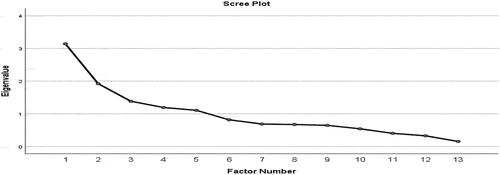
Table 3 reports the rotated factors, their loading, and their unique variance. As shown, this study finds five dimensions of PI. Considering the variables with loading ≥.32, the first factor has high loadings on successful coups, riots, and the number of major constitutional changes named instability of the political regime. The second factor has high loadings on guerrilla warfare and ethnic warfare named as war. The third factor has high loadings on the number of major cabinet changes, changes in effective executive, and the number of legislative elections named government instability. The fourth factor with high loadings on assassinations, government crises, and revolutions named aggression (1). And the fifth factor has high loadings on anti-government demonstrations, and alleged Coups is named aggression (2). The general strike and purges indicators did not load on any factors, so they are removed from the analysis.

Table 3. Factor-loading matrix and unique variances estimates

Factors
	Instability of the political regime	War	Government instability	Aggression (1)	Aggression (2)	Unique Variance
Riots	.834	.131	.092	−.041	.277	0.20
Successful Coups	.588	.003	−.101	.087	−.104	0.63
Number of Major Constitutional Changes	.511	−.064	.078	.052	−.067	0.72
Guerrilla Warfare	.100	.846	−.022	.057	−.127	0.25
ethnic warfare	−.032	.713	.022	.038	.119	0.47
Number of Major Cabinet Changes	.012	−.103	.920	.012	−.072	0.14
Changes in Effective Executive	.278	.056	.448	.009	−.167	0.69
Number of Legislative Elections	−.078	.041	.411	.033	.068	0.82
Assassinations	−.090	.189	−.048	.717	−.015	0.44
Government Crises	−.006	.063	.141	.579	.044	0.64
Revolutions	.197	−.171	−.013	.413	.042	0.76
Anti-Government Demonstrations	.604	.016	.165	−.077	.643	0.19
Alleged Coup	−.032	.000	−.026	.043	.348	0.88

Extraction Method: Maximum Likelihood.

Rotation Method: Oblimin with Kaiser Normalization.

3.2. Inflation volatility measurement

This research aims to estimate the conditional volatility of the inflation rate by employing three GARCH models (GARCH, TGARCH, and EGARCH) for each country. For this purpose, it used monthly time series of the CPI for the 14 MENA countries from January 2006 until December 2018. Table 4 provides descriptive statistics of the selected monthly inflation by country. Most of the inflation rates in the selected countries are positively skewed and reported high values of kurtosis, which indicates that the series has followed a leptokurtic distribution. However, GARCH models easily replicates the fat tails (leptokurtic) in the inflation series data. The augmented Dickey–Fuller unit-root test strongly rejects the null hypothesis that the inflation series have a unit root for all the countries. The Jarque—Bera statistic test rejects the null hypothesis that the inflation series is normally distributed for most countries. In addition, the ARCH test for heteroscedasticity rejects the null hypothesis that the error variance is homoscedastic for most of the countries. Accordingly, these diagnostic tests suggested the existence of the ARCH effect on the selected inflation series; therefore, they are suitable for modeling in the ARCH family process.

Table 4. Descriptive statistics of the selected monthly inflations by country

	Mean	Median	Std. Dev	Skew	Kurt.	Lag^1	Unit root test		Normality test		Heteroscedasticity^4
							ADF^2	p-value	JB^3	p-value	F-test	p-value
Algeria	0.391	0.455	0.885	−0.022	2.846	4	−9.880	0.000***	0.166	0.920	4.597	0.034**
Bahrain	0.251	0.255	0.663	−1.197	8.480	3	−12.203	0.000***	233.300	0.000***	4.336	0.001***
Djibouti	0.261	0.338	0.930	−0.590	6.903	5	−4.678	0.000***	108.638	0.000***	7.951	0.005***
Egypt	0.996	0.990	1.143	0.171	2.902	1	−7.670	0.000***	16.056	0.000***	3.608	0.059*
Iran	1.450	1.217	1.197	1.631	6.707	3	−3.037	0.034**	158.262	0.000***	18.079	0.000***
Iraq	0.274	0.177	0.926	0.582	4.574	12	−3.845	0.017**	24.911	0.000***	17.186	0.000***
Israel	0.120	0.101	0.412	0.224	3.363	17	−4.430	0.003**	2.154	0.341	2.123	0.027**
Jordan	0.304	0.260	0.828	1.619	18.40	10	−9.392	0.000***	1618.900	0.000***	0.053	0.818
Kuwait	0.306	0.171	0.459	1.539	6.627	10	−3.761	0.021**	146.480	0.000***	4.451	0.037**
Morocco	0.126	0.148	0.609	−0.005	3.302	4	−10.647	0.000***	4.217	0.121	26.961	0.000***
Oman	0.248	0.171	0.456	0.812	3.793	4	−6.185	0.000***	21.550	0.000***	7.043	0.009***
Saudi Arabia	0.273	0.184	0.517	3.211	22.12	1	−10.344	0.000***	2655.700	0.000***	0.332	0.566
Tunisia	0.364	0.356	0.298	−0.026	2.883	2	−6.101	0.000***	0.106	0.948	0.047	0.829
United Arab Emirates	0.238	0.113	0.753	6.697	65.08	0	−10.643	0.000***	26365.5	0.000***	4.285	0.040**

1. The optimal lag length obtained from the standard VAR model, based on Akaike information criterion. 2. ADF denotes coefficient of augmented Dickey-Fuller unit-root test performed with every country optimal lag. 3. JB denotes coefficient of Jarque-Bera of normality. 4. Based on ARCH test (Squared Lagged Residuals)* Statistical significance at 1% level.** Statistical significance at 5% level.*** Statistical significance at 10% level.

After applying GARCH models, the best-fitted model has been chosen by comparing three benchmark indicators: the Akaike Information Criterion (AIC) and Schwarz Information Criterion (SIC), ARCH Lagrange Multiplier (LM) test, and serial correlation test (Correlogram of Standardized Residuals Squared). Strong indicators were the AIC and SIC, while the ARCH LM test was used due to the GARCH process employment. The ARCH LM results show whether an ARCH effect is still present in the inflation series after applying the GARCH model or not.

According to Table 5, the relatively high p-value for the ARCH LM test suggests that GARCH parameterization is appropriate for the conditional variance processes for all models. In addition, the serial correlation test (Correlogram of Standardized Residuals Squared) for lag (12) was chosen to confirm that there is no serial correlation in the residuals, Table 5 shows an insignificant p-value for all models. The decision about the most favorable model for creating conditional variance is based on the model with the lowest AIC and SIC values. The optimal model was consequently utilized for the creation of the IV series. Regarding Table 5, the current study follows Rizvi and Naqvi (2009) findings that asymmetric models are more prevalent than symmetric ones. TGARCH is the most prevalent model, it is the best-fitted model for seven countries (Algeria, Iran, Israel, Jordan, Oman, Saudi Arabia, Tunisia). EGARCH model is the best-fitted model for five countries (Djibouti, Iraq, Kuwait, Morocco, UAE). Meanwhile, just two countries (Bahrain and Egypt) have GARCH as the best-fitted model. The monthly conditional volatility is created based on the best-fitted model for each country. After that, to turn the monthly data into annual data points, this study considers the average of monthly conditional volatility within each year to be annual conditional volatility for that year.

Table 5. An overview of three country-specific conditional variance specifications and the best fitted model

	GARCH (1,1)				TGARCH (1,1)				EGARCH (1,1)
	AIC^1 SC^2	ARCH^3 F-test P-value	Q^2(12)^4 Q-stat P-value	JB^5	AIC SC	ARCH F-test P-value	Q^2 (12) Q-stat P-value	JB	AIC SC	ARCH F-test P-value	Q^2(12) Q-stat P-value	JB
Algeria	2.633 2.731	0.191 0.662	10.29 0.590	0.488 0.784	2.607 2.724	0.657 0.418	15.224 0.229	0.639 0.726	2.653 2.771	0.1702 0.6805	7.085 0.852	0.152 0.926
Bahrain	2.012 2.110	0.083 0.772	2.526 0.998	185.09	2.037 2.154	0.754 0.098	2.335 0.999	187.75	2.021 2.139	0.1895 0.6635	4.3811 0.976	136.906
Djibouti	2.415 2.513	0.382 0.537	6.776 0.872	11.253	2.399 2.516	0.4491 0.5038	5.934 0.919	23.795	2.382 2.500	0.8612 0.3548	6.819 0.869	18.983
Egypt	2.617 2.715	1.336 0.249	13.24 0.352	8.060 .017	2.704 2.821	3.5E07 0.9995	7.782 0.802	13.905	2.734 2.832	3.86E–05 0.995	8.880 0.713	13.23
Iran	2.655 2.753	0.190 0.663	13.83 0.312	38.211	2.562 2.679	0.0296 0.8635	8.003 0.785	12.580	2.666 2.764	0.0033 0.9538	19.377 0.080	15.0537
Iraq	2.475 2.573	0.9099 0.3416	12.22 0.428	7.8797	2.4609 2.5782	1.6328 0.2032	13.582 0.328	10.268	2.439 2.5570	1.2584 0.2637	14.307 0.282	14.84
Israel	0.9895 1.0873	0.0052 0.9423	11.97 0.152	0.5517 0.578	0.9156 1.0329	2.9335 0.0888	9.9900 0.125	0.086 0.957	0.9891 1.0869	0.0156 0.9005	11.767 0.162	1.429 0.489
Jordan	2.389 2.487	0.1385 0.7102	2.4365 0.998	920.19	2.3730 2.4904	0.0762 0.7828	3.269 0.993	742.66	2.397 2.495	0.0990 0.7534	9.8391 0.364	840.6
Kuwait	1.0757 1.1734	0.0052 0.9421	10.427 0.236	34.680	1.068 1.186	0.1548 0.6944	12.365 0.136	27.888	1.061 1.159	0.0034 0.9530	10.013 0.264	32.368
Morocco	1.6817 1.7795	0.0172 0.8958	15.746 0.203	1.622 0.444	1.694 1.811	0.0185 0.8918	15.7 0.204	1.558 0.458	1.678 1.796	3.9E–05 0.9950	13.609 0.326	0.1512 0.927
Oman	1.1551 1.2528	0.3940 0.5311	8.4371 0.750	5.621 0.601	1.102 1.220	1.1913 0.2768	4.5013 0.973	5.915 0.051	1.1381 1.2359	0.1814 0.6708	8.0915 0.778	4.474 0.107
Saudi Arabia	1.3881 1.4858	0.5452 0.4614	2.3024 0.999	595.40	1.0714 1.1887	0.1974 0.6574	5.0026 0.958	111.65	1.2096 1.3269	7.6E–05 0.9930	3.5748 0.990	160.912
Tunisia	0.4514 0.5491	0.0032 0.9546	11.464 0.177	0.2906 0.8647	0.4165 0.5338	0.2756 0.6003	11.689 0.166	0.5253 0. 7687	0.4514 0.5491	0.00324 0.9546	11.464 0.177	0.2906 0.864
UAE	2.2099 2.3076	0.0070 0.9332	0.2154 1.000	27347.11	2.1708 2.2881	0.0048 0.9446	0.1842 1.000	28771.0	1.4713 1.5886	0.0900 0.7646	1.3143 1.000	235.622

1. Akaike info criterion; 2. Schwarz criterion; 3. ARCH(LM) heteroscedasticity test; 4. Q2 (12) stat is the value of the serial correlation test (Correlogram of Standardized Residuals Squared) for lag (12). 5. JB is Jarque-Bera coefficient for residuals normality.

3.3. The impact of political instability on inflation volatility

3.3.1. Summary statistics and correlation

Table 6 presents a summary statistic for the key variables. GARCH models generate IV values, so the IV values reported in Table 6 represent the conditional volatility of the inflation rate. The average IV is 0.51%, and the average inflation level is 5.12%. The only very high inflation rate value, 53.23%, was recorded in Iraq in 2006. However, the countries that recorded inflation values more than 20% including, Iran 2013 (36.60%), Egypt 2017 (29.50%), Iran 2012, 2011, 2008 (27.25%, 26.29%, 25.41%, respectively). The data of the PI variables are obtained from the FA technique; therefore, the summary statistics of PI variables presented the factor score values.

Table 6. Summary statistics for key variables

Key variable	Obs.	Mean	Std.Dev.	Min.	Max.
IV	182	.5150494	.5570621	.0193857	4.808562
Inflation	182	5.12236	6.767664	−10.06749	53.23096
Region instability	182	−1.65e-06	1	−.9646	9.03138
War	182	1.48e-06	.9999997	−.93254	7.5968
Government instability	182	4.95e-07	.9999997	−.97002	3.96491
Aggression (1)	182	9.34e-07	.9999998	−1.07905	9.11597
Aggression (2)	182	1.39e-18	.9999998	−3.05457	6.75257
Polity scale	182	−3.472527	5.306809	−10	7
GDP	182	4.285198	.388239	3.613203	4.980813
Agriculture	182	4.873714	4.412221	.160021	13.86911
Trade	182	105.4626	61.14154	30.24655	347.9965
Board money	182	3.440943	3.350476	0	16.47424

Table 7 shows the correlation matrix for the key variables, inflation level is positively correlated with IV, which confirmed the Friedman-Ball’s theory that increase in the rate of inflation rise the IV. The correlation coefficients between the various PI indicators are low and go in two directions (+, -). The correlation coefficients between PI indicators and IV are relatively low and positive, except the government instability and aggression (2) dimensions are negative. Agriculture, trade, and broad money are positively correlated with IV, while GDP is negatively correlated with IV.

Table 7. Correlation matrix

Key variable	IV	l. IV	Inflation	Region instability	War	Government instability	Aggression (1)	Aggression (2)	Polity	GDP	Agriculture	Trade	Broad money
IV	1.0000
l. IV	0.4493	1.0000
Inflation	0.3562	0.2948	1.0000
Region Instability	0.0955	0.0506	0.0998	1.0000
War	0.0389	0.0622	−0.0793	0.0000	1.0000
Government Instability	−0.096	−0.108	−0.0565	0.0000	−0.000	1.0000
Aggression (1)	0.1120	0.1661	0.3997	0.0000	−0.000	−0.000	1.0000
Aggression (2)	−0.090	−0.070	0.0332	0.0000	−0.000	−0.000	−0.000	1.0000
Polity scale	0.0735	0.1017	−0.1268	−0.061	0.3725	0.2095	0.0435	−0.015	1.0000
GDP	−0.326	−0.338	−0.1330	−0.112	−0.064	0.0230	−0.125	0.0401	−0.492	1.0000
Agriculture	0.1863	0.1791	0.2909	0.2654	−0.028	−0.017	0.083	0.003	0.1453	−0.632	1.0000
Trade	0.0290	0.0301	−0.2443	−0.141	−0.148	−0.096	−0.112	−0.070	0.0622	−0.132	−0.495	1.0000
Broad money	0.3664	0.3425	0.4384	0.0381	−0.158	−0.131	0.2697	−0.030	−0.209	−0.028	0.1212	−0.142	1.000

3.4. The main results

For all models in Tables (8, 9, B.1-B.3),⁶ the estimation results reported are run by the system-GMM estimator. All the right-hand side variables are instrumented, but too many instruments may bias the results because the number of instruments may exceed the number of countries. To avoid over fitting of instruments, the current study collapsed the instrument set (Roodman, 2009).⁷ Also, the smallest possible lags lengths are used; twice-lagged values of the dependent and all explanatory variables in the first-difference equations and their once-lagged first-differences are used in the level equation.

Table 8. The impact of PI on IV

	(1)	(2)	(3)	(4)	(5)	(6)	(7)
L.IV	0.223**	0.231**	0.212**	0.214**	0.231**	0.226**	0.189**
	(0.0949)	(0.0895)	(0.0929)	(0.0775)	(0.0916)	(0.0853)	(0.0768)
Inflation	0.0398***	0.0399***	0.0399***	0.0399***	0.0396***	0.0389***	0.0394***
	(0.0107)	(0.0109)	(0.0107)	(0.00992)	(0.0107)	(0.0109)	(0.00976)
Regime instability	0.0284**						0.0274**
	(0.0126)						(0.0126)
War		0.0110					0.0157
		(0.0344)					(0.0325)
Government instability			−0.0608**				−0.0595*
			(0.0276)				(0.0277)
Aggression (1)				0.0848			0.0873
				(0.0635)			(0.0617)
Aggression (2)					−0.0229		−0.0131
					(0.0280)		(0.0284)
Polity scale						−0.00715	−0.00477
						(0.00932)	(0.00974)
GDP	−0.555***	−0.523**	−0.584***	−0.495***	−0.536***	−0.636**	−0.589**
	(0.167)	(0.186)	(0.175)	(0.152)	(0.164)	(0.238)	(0.225)
Agriculture	−0.0313	−0.0270	−0.0317	−0.0250	−0.0284	−0.0337	−0.0318
	(0.0205)	(0.0216)	(0.0204)	(0.0200)	(0.0198)	(0.0234)	(0.0242)
Trade	−0.000130	1.23e-05	−0.000334	0.000221	−0.000117	−0.000344	−8.68e-05
	(0.000987)	(0.00116)	(0.000922)	(0.000787)	(0.000967)	(0.00114)	(0.000867)
Constant	2.761***	2.584**	2.911***	2.443***	2.661***	3.121**	2.908**
	(0.872)	(0.985)	(0.902)	(0.761)	(0.848)	(1.193)	(1.107)
Observations	168	168	168	168	168	168	168
Groups	14	14	14	14	14	14	14
Instr.	9	9	9	9	9	9	14
Hansen	0.578	0.596	0.664	0.536	0.581	0.572	0.633
AB AR(1)	0.194	0.193	0.184	0.195	0.193	0.172	0.157
AB AR(2)	0.129	0.121	0.152	0.194	0.116	0.121	0.208

Note: Robust standard errors in parentheses (*** p<0.01, ** p<0.05, * p<0.1)

Table 9. The impact of PI on IV controlling for broad money

	(1)	(2)	(3)	(4)	(5)	(6)	(7)
L.IV	0.207**	0.214**	0.200**	0.205**	0.215**	0.214**	0.183**
	(0.0841)	(0.0860)	(0.0903)	(0.0768)	(0.0826)	(0.0815)	(0.0835)
Inflation	0.0317***	0.031***	0.032***	0.032***	0.031***	0.031***	0.0326***
	(0.0103)	(0.0104)	(0.0106)	(0.0093)	(0.0104)	(0.0103)	(0.00954)
Regime instability	0.0282*						0.0276*
	(0.0138)						(0.0132)
War		0.0245					0.0256
		(0.0193)					(0.0278)
Government instability			−0.0438*				−0.0456*
			(0.0239)				(0.0231)
Aggression (1)				0.0529			0.0569
				(0.0484)			(0.0481)
Aggression (2)					−0.0221		−0.0155
					(0.0319)		(0.0317)
Polity scale						−0.00239	−0.00251
						(0.0067)	(0.00906)
GDP	−0.549***	−0.529***	−0.55***	−0.53***	−0.53***	−0.56***	−0.563***
	(0.146)	(0.141)	(0.157)	(0.137)	(0.142)	(0.161)	(0.177)
Agriculture	−0.0294*	−0.0266	−0.0272	−0.0275	−0.0267	−0.0278	−0.0295
	(0.0163)	(0.0156)	(0.0162)	(0.0157)	(0.0159)	(0.0166)	(0.0180)
Broad money	0.0118**	0.0121**	0.0112**	0.0108**	0.0117**	0.0115**	0.0104**
	(0.00499)	(0.00514)	(0.00501)	(0.0043)	(0.0050)	(0.0049)	(0.00445)
Constant	2.623***	2.520***	2.626***	2.555***	2.534***	2.657***	2.701***
	(0.671)	(0.648)	(0.727)	(0.625)	(0.653)	(0.728)	(0.804)
Observations	168	168	168	168	168	168	168
Groups	14	14	14	14	14	14	14
Instr.	9	9	9	9	9	9	14
Hansen	0.298	0.290	0.381	0.360	0.277	0.290	0.358
AB AR(1)	0.162	0.160	0.159	0.173	0.164	0.167	0.160
AB AR(2)	0.115	0.101	0.135	0.116	0.099	0.108	0.139

Note: Robust standard errors in parentheses (*** p<0.01, ** p<0.05, * p<0.1).

All the models reported in all tables are well specified, and the estimator chosen is appropriate since the diagnostics in all tables are all satisfactory. Particularly, the Hansen test was insignificant, and the null hypothesis of endogenous instruments can be rejected in all the models. Additionally, Arellano and Bond (1991) test results reported no serial correlation in the second lag of the error in all models. Heteroskedastic standard errors are reported in all models. In addition, the coefficient of the first lag of the dependent variable is positive and highly significant in all the models in all tables. This result can be interpreted as, if inflation is volatile today, it will be more volatile tomorrow. The inflation level is positive and high significant in all the models, indicating that high inflation tends to be very volatile, confirming Friedman-Ball’s theory (Ball, 1992).

Table 8 presents the estimation results of the impact of PI on IV. As expected, the instability of the political regime dimension reported significant positive results in model 1 and model 7. A unit increase in this dimension increases the IV by about 0.028%. On the other hand, the government instability dimension reported statistically significant negative results in model 3 and model 7. A unit increase in this dimension decreases IV by about 0.060%, while the other PI dimensions reported non-significant results. Also, the polity scale reported a non-significant negative impact on IV which means, the more the MENA region moves towards a more democratic form of government, it does not significantly reduce IV. Turning to other economic variables, as expected, all of them negatively affect the IV; however, the results were significant for the real GDP level per capita only.

For the role of the Broad Money. Table 9 reports the results for considering the monetary variable “broad money.” As the table illustrates, as expected, broad money has a significant positive impact on IV in all models. That means a unit increase in the money supply rises IV by about 10–12%. This result is in line with all the previous studies that tested the impact of PI on inflation and IV (Aisen & Veiga, 2006, 2008; Barugahara, 2015; Khan et al., 2011; Telatar et al., 2010). Comparing the results of the other variables with Table 8, all the results reported in Table 9 have the same sign and significance. Therefore, the PI effect is robust to the inclusion of the broad money.

4. Other robustness checks

4.1. Using the standard deviation

The study uses an alternative measure of IV. Table B.1 provides the results of using the standard deviation of inflation level instead of the GARCH models. As shown, the coefficient of inflation and log of IV are positive and highly significant as expected for all models. Comparing the results of the PI dimensions with Table 8, all the signs are the same. The instability of the political regime is positively significant in model 7 only. In addition, government instability is negatively significant in model 7 only. Unlike Table 8, the war indicator is negatively significant, and the aggression (1) indicator is positively significant in models 2 and 4; however, they were insignificant in model 7. The GDP per capita results are insignificant for models 1 to 6 but became significant in model 7. The agriculture and trade have the same results as in Table B.1. The constants for all models are insignificant except the result of model 7. The weakening in GDP per capita results may be because the standard deviation is not the optimal measure of IV. This gives credit to the conditional variance method as a better measure of IV. However, considering model 7, where all the PI included in the same regression, the PI’s impact on IV is robust to an alternative measure of IV.

Aisen and Veiga (2008) is the only study that used standard deviation to measure the IV in studying the impact of PI on IV. Aisen and Veiga (2008) used some of the PI indicators that we used in this study such as (assassination, coups, cabinet changes) and reported a positive impact of all PI indicators on IV.

4.2. Using the MIDAS weights

This study also employs MIDAS weights to estimate the annual IV from the monthly conditional variance of IV obtained from the GARCH models instead of simple averaging. The current research calculates the annual IV for each country using Beta lags weight through MSE cross-validation procedure. Table B.2 report the results of the impact of PI on IV using Beta lags weight.⁸ Comparing the results with Table 8, all the results reported in Table B.2 had similar signs and significance levels. Therefore, previous conclusions on the impact of PI on IV for simple averaging of GARCH conditional variance IV hold for MIDAS weight and are robust.

4.3. Using the two-stage regression strategy

This study uses the two-stage regression strategy to identify the PI variables that truly affect the IV. The first-stage estimation starts with estimating the general model containing all the used variables to determine the variable’s significance by entering the PI dimensions one by one. The significant variables identified from the first-stage analysis are considered in the second-stage estimation, and the model is re-estimated. This two-stage regression strategy is expected to provide sufficiently strong evidence for the impact of PI dimension on the IV. Table B.3 reported the results from these estimations. It shows that, in the general model that used regime instability dimension as PI indicator, the coefficient of the first lag of IV is positive and highly significant, and the coefficient of the regime instability indicator is positive and significant, as expected. Other control variables are robust to the results reported in the previous tables. In the specific model (model 2), the importance of the significant variables in the general model are further tested. And finds that all the significant variables in model 1 are still significant. Considering the models of estimation government instability indicator, in the general model (model 1), the coefficient of the first lag of the IV is positive and highly significant. The coefficient of the government instability indicator is negative and significant, as expected. Other variables are robust to the results reported in Tables 8, 9. In the specific model (model 2), the importance of the significant variables in the general model 1 is tested again. However, model 2 reported that all the significant variables in model 1 are still significant. While looking at war, aggression (1), aggression (2), and polity scale indicator’s estimations. All the PI indicators did not report significant results. As expected, the first lag of the IV, inflation, GDP per capita, and broad money are the only variables that reported significant results.

To conclude, the results for the impact of PI on IV are robust to the inclusion of broad money. Also, these results are valid by applying robustness checks, using alternative measures of IV, and using two-stage regression analysis. To conclude, regime instability, government instability, inflation, GDP per capita, and broad money variables are the most important determinations of the IV in the MENA region.

5. Discussion

We find evidence that, as one might expect, the instability of the political regime (i.e., riots, coups, and major constitutional changes) is positively related to IV. These results are in line with Barugahara (2015). In contrast, and somewhat surprisingly, we find evidence that government instability may actually reduce IV. This measure of PI includes the number of major cabinet changes, changes in effective executive and the number of legislative elections. This result contrasts with previous research finding a positive relationship between the number of major cabinet changes and inflation (Aisen & Veiga, 2006; Khan et al., 2011) or with IV Aisen and Veiga (2008). This difference could be down to our improved measure of PI, the more recent time period, the more advanced techniques or our focus on the MENA region. While this result is somewhat counter-intuitive, ours is not the only study to identify the possibility of a positive effect from PI. For instance, Jong-A-Pin (2009) find evidence that PI of the political regime can increase economic growth. This finding also supported the model of Besley et al. (2005), in which political competition is good for economic performance since incompetent politicians can be more readily held accountable for the implementation of inappropriate government policies.

These results could also be explained by our focus on the MENA region. As (Aisen & Veiga, 2006, 2008) discuss more frequent cabinet changes shorten the scope of the government's since every new cabinet that takes power might not be sure that they will be in their posts for the whole period; therefore, they are concerned about the short-term objectives rather than working on a coherent and comprehensive economic plan. But this is perhaps not the case for the MENA region. For example, following the Arab Spring in Egypt, Mohmed Morsi was the first democratically elected president after Mubarak’s rule, which lasted about 29 years. During Mubarak’s regime, characterised by a high degree of corruption and favouritism, large portions of the population were excluded from jobs and political participation. Morsi had appointed a more qualified government away from corruption, favouritism, and nepotism (Habibi, 2012). Accordingly, this government implemented better monetary and fiscal policies. For example, in December 2012, after 7 months of Mohmed Morsi became president, inflation fell to its lowest rate in 20 years (about 7.11%).⁹

6. Conclusion

The main goal of this paper is to evaluate the links between PI and IV in the MENA region for the period from 2006 until 2018. By employing an advanced panel data estimation technique, the GMM method, this study reported strong evidence in favor of the view that PI has a significant effect on IV. The study finds that both the instability of the political regime and government instability are the most critical dimensions of PI in terms of influencing IV.

The only limitation of this study is the limited availability of data. Economic data for most countries were not available before 2006; therefore, the sample was selected according to the data availability. Also, six of the MENA region countries were excluded due to the lack of political and economic data (Lebanon, Libya, Qatar, Syria, West Bank and Gaza, and Yemen). Meanwhile, the inclusion of Libya, Syria, and Yemen would help us to establish a greater degree of accuracy because they experienced the Arab Spring revolution.

Correction

This article has been corrected with minor changes. These changes do not impact the academic content of the article.

Disclosure statement

No potential conflict of interest was reported by the authors.

Notes

1. See Figure 1.

2. See Table A1 for the list of economic variables are used.

3. For the full list of MENA region countries included in the study see Appendix A, Table A.3.

4. We selected the sample from 2006 due to the data availability, and through 2018 because we are not aimed to include the COVID-19 period that significantly affected the IV, we just examine the impact of PI only.

5. The data was collected for 18 PI indicators, but three indicators have no data (attempted coups, plotted coups, and civil warfare). So, they were excluded from the estimation.

6. See Appendix B.

7. Collapsing the instruments helps in creating one instrument for each variable and lag distance, rather than one for each time period, variable, and lag distance (Roodman, 2009).

8. Results for different MIDAS weighting schemes were also conducted but produce qualitatively similar results and are available upon request (See Figure C2).

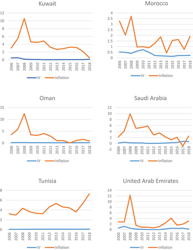
9. See Appendix C, Figure C1 for Inflation and IV Graph for Each Country.

Appendix

Appendix A: Country and Data Summary Tables

Table A1. List of Economic variables are used, definitions and sources

Indicator	Definition	Source
Inflation	Annual Percentage change in the consumer price index	International Monetary Fund (2020) World Bank (2020)
Income per capita	The real GDP per capita. We consider the income per capita indicator as it reflects the economic development of each nation. However, increasing in the GDP decreasing the inflation rate and thus its volatility.	World Bank (2020)
Trade openness	The ratio of total foreign trade relative to GDP. The literature suggested that more open economies lead to more diversity in consumption, which may reduce the sensitivity of consumer prices to price shocks in specific markets, therefore, decreasing IV.	World Bank (2020)
Broad money	The standard deviation of the annual growth rate of Broad Money (volatility of the money supply growth). Rises in the money supply will increase inflation and its volatility.	World Bank (2020)
The size of the Agriculture sector	Value-added of the Agriculture sector relative to GDP. We include the size of the agriculture sector indicator as it is considering as a measure of the shadow economy (informal sector). The literature suggested that the relationship between the agriculture sector and inflation rate is positive (Barugahara, 2015). But we expected a negative relationship depends on the fact that most of the MENA region counties do not have big agriculture sectors, except for the North African countries around the Mediterranean Sea, such as Tunisia, Morocco, and Egypt.	World Bank (2020)

Note: International Monetary Fund (2020) Data page https://data.imf.org/?sk=388dfa60-1d26-4ade-b505-a05a558d9a42

World Bank (2020) data page http://datatopics.worldbank.org/world-development-indicators/

Table A2. List of political indicators used, definitions, and sources

Indicator	Definition	Source
Anti-government Demonstrations	Any peaceful public gathering of at least 100 people for the primary purpose of displaying or voicing their opposition to government policies or authority, excluding demonstrations of a distinctly anti-foreign nature.	DataBanks International Cross-National Time-Series Data Archive
Assassinations	Any politically motivated murder or attempted murder of a high government official or politician.	DataBanks International Cross-National Time-Series Data Archive
General Strikes	Any strike of 1,000 or more industrial or service workers involves more than one employer and is aimed at national government policies or authority.	DataBanks International Cross-National Time-Series Data Archive
Terrorism/Guerrilla Warfare	Any armed activity, sabotage, or bombings carried on by independent bands of citizens or irregular forces and aimed at the overthrow of the present regime.	DataBanks International Cross-National Time-Series Data Archive
Major Government Crises	Any rapidly developing situation that threatens to bring the downfall of the present regime—excluding situations of revolt aimed at such overthrow.	DataBanks International Cross-National Time-Series Data Archive
Purges	Any systematic elimination by jailing or executing political opposition within the ranks of the regime or the opposition.	DataBanks International Cross-National Time-Series Data Archive
Revolutions	Any illegal or forced change in the top government elite, any attempt at such a change, or any successful or unsuccessful armed rebellion whose aim is independence from the central government.	DataBanks International Cross-National Time-Series Data Archive
Riots	Any violent demonstration or clash of more than 100 citizens involving the use of physical force.	DataBanks International Cross-National Time-Series Data Archive
Number of Major Constitutional Changes	Major Constitutional Changes The number of basic alterations in a state’s constitutional structure, the extreme case being the adoption of a new constitution that significantly alters the prerogatives of the various branches of government. Examples of the latter might be the substitution of presidential for parliamentary government or the replacement of monarchical by republican rule. Constitutional amendments which do not have a significant impact on the political system are not counted.	DataBanks International Cross-National Time-Series Data Archive
Number of Major Cabinet Changes	The number of times in a year that a new premier is named and/or 50% of the cabinet posts are assumed by new ministers.	DataBanks International Cross-National Time-Series Data Archive
Executive Changes	The number of times in a year that effective control of executive power changes hands. Such a change requires that the new executive be independent of his predecessor.	DataBanks International Cross-National Time-Series Data Archive
Number of Legislative Elections	The number of elections held for the lower house of a national legislature in a given year. A limited number of by-elections are included, but most are not.	DataBanks International Cross-National Time-Series Data Archive
Successful Coups	The Number of successful coups d’Etat that occurred in the year of record	Integrated Network for Societal Conflict Research (INSCR)
Attempted Coups	The Number of attempted (but ultimately unsuccessful) coups d’Etat that occurred in the year of record	Integrated Network for Societal Conflict Research (INSCR)
Plotted Coups	The Number of (thwarted) coup plots that were reported by government officials during the year of record	Integrated Network for Societal Conflict Research (INSCR)
Alleged Coup Plots	The Number of alleged coup plots announced by government officials during the year of record (allegations of coup plots usually involve less formal adjudication procedures and are often used by authorities to justify repression of opposition leaders)	Integrated Network for Societal Conflict Research (INSCR)
Civil Warfare	The number of civil warfare involving that state in that year	Integrated Network for Societal Conflict Research (INSCR)
Ethnic Warfare	The number of ethnic warfare involving that state in that year	Integrated Network for Societal Conflict Research (INSCR)
Polity scale	From strongly democratic (+10) to strongly autocratic (−10)	Integrated Network for Societal Conflict Research (INSCR)

Note: h A. 2020. Cross-National Time-Series Data Archive. Databanks International. Jerusalem, Israel; see https://www.cntsdata.com/

Integrated Network for Societal Conflict Research (INSCR) Data page, http://www.systemicpeace.org/inscrdata.html

Table A3. List of the MENA countries included in the study

Algeria	Bahrain
Djibouti	Egypt
Iran	Iraq
Israel	Jordan
Kuwait	Morocco
Oman	Saudi Arabia
Tunisia	United Arab Emirates

Appendix B: The Result Tables for the Impact of PI on IV

Table B1. The Impact of PI on IV Using Standard Deviation of Inflation as Measure of IV

	(1)	(2)	(3)	(4)	(5)	(6)	(7)
L.IV	0.403***	0.427***	0.403***	0.433***	0.407***	0.411***	0.0225*
	(0.0315)	(0.0353)	(0.0307)	(0.0382)	(0.0308)	(0.0363)	(0.0110)
Inflation	0.456***	0.457***	0.454***	0.453***	0.455***	0.457***	0.0404***
	(0.0934)	(0.0918)	(0.0935)	(0.0895)	(0.0925)	(0.0969)	(0.00825)
Region instability	0.0818						0.0319*
	(0.135)						(0.0167)
War		0.445***					0.0259
		(0.108)					(0.0345)
Government instability			−0.255				−0.0600**
			(0.209)				(0.0251)
Aggression (1)				0.861***			0.0531
				(0.197)			(0.0511)
Aggression (2)					−0.0382		−0.0281
					(0.281)		(0.0325)
Polity scale						−0.0173	−0.000796
						(0.0655)	(0.0134)
GDP	−0.881	−0.198	−1.045	−1.387	−0.895	−0.662	−0.602**
	(0.840)	(0.829)	(0.738)	(0.927)	(0.816)	(1.121)	(0.261)
Agriculture	−0.157	−0.0958	−0.176	−0.199	−0.164	−0.151	−0.0304
	(0.151)	(0.148)	(0.139)	(0.136)	(0.146)	(0.133)	(0.0289)
Trade	−0.00237	0.00219	−0.00346	−0.00504	−0.00244	−0.00169	0.000386
	(0.0046)	(0.0052)	(0.0043)	(0.00461)	(0.0046)	(0.0043)	(0.000920)
Constant	4.846	1.026	5.761	7.354	4.935	3.828	2.921**
	(4.335)	(4.472)	(3.800)	(4.680)	(4.207)	(5.328)	(1.255)
Observations	168	168	168	168	168	168	168
Groups	14	14	14	14	14	14	14
Inst.	9	9	9	9	9	9	14
Hansen	0.277	0.277	0.341	0.399	0.127	0.244	0.486
AB AR(1)	0.021	0.021	0.021	0.021	0.016	0.021	0.174
AB AR(2)	0.879	0.879	0.674	0.628	0.863	0.813	0.204

Note: Robust standard errors in parentheses (*** p < 0.01, ** p < 0.05, * p < 0.1).

Table B2. The Impact of PI on IV with annualised IV by using Beta lags (MIDAS weight)

	(1)	(2)	(3)	(4)	(5)	(6)	(7)
L.IV	0.211*	0.220*	0.199	0.200*	0.220*	0.215*	0.174*
	(0.114)	(0.108)	(0.113)	(0.0929)	(0.110)	(0.104)	(0.0943)
Inflation	0.0392***	0.0393***	0.0393***	0.0393***	0.0389***	0.0383***	0.0390***
	(0.0101)	(0.0103)	(0.0101)	(0.00928)	(0.0101)	(0.0103)	(0.00916)
Regime instability	0.0269*						0.0260*
	(0.0131)						(0.0129)
War		0.0133					0.0178
		(0.0364)					(0.0342)
Government instability			−0.0567*				−0.0564*
			(0.0277)				(0.0276)
Aggression (1)				0.0890			0.0923
				(0.0629)			(0.0620)
Aggression (2)					−0.0202		−0.0101
					(0.0285)		(0.0288)
Polity scale						−0.00615	−0.00404
						(0.00954)	(0.01000)
GDP	−0.532***	−0.497**	−0.560***	−0.470***	−0.514***	−0.600**	−0.550**
	(0.160)	(0.178)	(0.166)	(0.140)	(0.156)	(0.237)	(0.218)
Agriculture	−0.0286	−0.0240	−0.0290	−0.0223	−0.0259	−0.0304	−0.0279
	(0.0202)	(0.0213)	(0.0199)	(0.0194)	(0.0194)	(0.0235)	(0.0237)
Trade	−3.43e-05	0.000128	−0.000223	0.000331	−2.02e-05	−0.000214	9.08e-05
	(0.00101)	(0.00119)	(0.000957)	(0.000796)	(0.000990)	(0.00118)	(0.000893)
Constant	2.643***	2.449**	2.789***	2.318***	2.547***	2.944**	2.712**
	(0.848)	(0.956)	(0.868)	(0.713)	(0.823)	(1.198)	(1.080)
Observations	168	168	168	168	168	168	168
Groups	14	14	14	14	14	14	14
Instr.	9	9	9	9	9	9	14
Hansen	0.667	0.688	0.759	0.587	0.657	0.650	0.725
AB AR(1)	0.147	0.146	0.136	0.146	0.146	0.150	0.131
AB AR(2)	0.192	0.171	0.230	0.262	0.150	0.164	0.334

Note: Robust standard errors in parentheses (*** p < 0.01, ** p < 0.05, * p < 0.1).

Table B3. The impact of PI on IV from a General Model to Specific Model

	Regime instability		War	Government instability		Aggression (1)	Aggression (2)	Polity scale
	Model 1	Model 2		Model 1	Model 2
L.IV	0.246***	0.224***sss	0.253***	0.215**	0.234**	0.244***	0.250***	0.252***
	(0.0737)	(0.0697)	(0.0762)	(0.0781)	(0.0838)	(0.0630)	(0.0736)	(0.0705)
Regime ins.	0.0279*	0.0281*
	(0.0133)	(0.0135)
War			0.0288
			(0.0251)
Government instability				−0.0445*	−0.0441*
				(0.0244)	(0.0230)
Aggression (1)						0.0526
						(0.0459)
Aggression (2)							−0.0214
							(0.0303)
Polity scale								−0.00287
								(0.00782)
Inflation	0.0301**	0.031***	0.0301**	0.032***	0.0264**	0.030***	0.0300**	0.0299**
	(0.0100)	(0.0102)	(0.0102)	(0.0105)	(0.0089)	(0.0088)	(0.0101)	(0.0101)
GDP	−0.52***	−0.53***	−0.472**	−0.56***	−0.34***	−0.48***	−0.51***	−0.553**
	(0.161)	(0.138)	(0.165)	(0.186)	(0.109)	(0.153)	(0.160)	(0.215)
Agriculture	−0.0284		−0.0215	−0.0294		−0.0237	−0.0257	−0.0278
	(0.0194)		(0.0190)	(0.0205)		(0.0191)	(0.0187)	(0.0219)
Trade	−6.12e-0		0.000245	−0.00019		0.000166	−5.01e-0	−0.000126
	(0.0008)		(0.0008)	(0.0007)		(0.0007)	(0.0008)	(0.000945)
Broad money	0.0111**	0.0116**	0.0115**	0.0109**	0.0109*	0.0101**	0.0111**	0.0108**
	(0.0048)	(0.0050)	(0.0049)	(0.0049)	(0.0053)	(0.0043)	(0.0048)	(0.00472)
Constant	2.534***	2.574***	2.215**	2.713**	1.647***	2.315***	2.451***	2.630**
	(0.801)	(0.634)	(0.819)	(0.920)	(0.494)	(0.747)	(0.790)	(1.053)
Observations	168	168	168	168	168	168	168	168
Country	14	14	14	14	14	14	14	14
Ins.	11	10	11	11	10	11	11	11
Hansen	0.425	0.421	0.439	0.502	0.555	0.383	0.399	0.420
AB AR(1)	0.168	0.169	0.162	0.164	0.162	0.177	0.167	0.170
AB AR(2)	0.102	0.130	0.107	0.152	0.159	0.133	0.109	0.117

Note: Robust standard errors in parentheses (*** p < 0.01, ** p < 0.05, * p < 0.1).

Appendix C: Inflation and IV Graphs

Figure C1. Inflation rate for the MENA region versus the rest of the World.

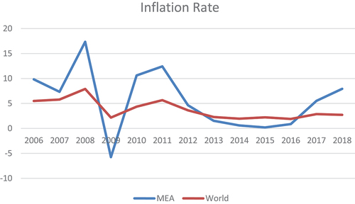
Figure C2. Inflation and IV graph for each country.

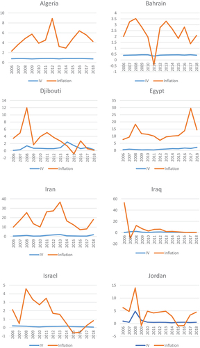
Figure C2. Continued.

References

- Aisen, A., & Veiga, F. J. (2006). Does political instability lead to higher inflation? A panel data analysis. Journal of Money, Credit, and Banking, 38(5), 1379–32. https://doi.org/10.1353/mcb.2006.0064
- Aisen, A., & Veiga, F. J. (2008). Political instability and inflation volatility. Public Choice, 135(3–4), 207–223. https://doi.org/10.1007/s11127-007-9254-x
- Aisen, A., & Veiga, F. J. (2013). How does political instability affect economic growth? European Journal of Political Economy, 29, 151–167. https://doi.org/10.1016/j.ejpoleco.2012.11.001
- Alesina, A., Özler, S., Roubini, N., & Swagel, P. (1996). Political instability and economic growth. Journal of Economic Growth, 1(2), 189–211. https://doi.org/10.1007/BF00138862
- Arellano, M., & Bond, S. (1991). Some tests of specification for panel data: Monte Carlo evidence and an application to employment equations. The Review of Economic Studies, 58(2), 277–297. https://doi.org/10.2307/2297968
- Ball, L. (1992). Why does high inflation raise inflation uncertainty? Journal of Monetary Economics, 29(3), 371–388. https://doi.org/10.1016/0304-39329290032-W
- Barugahara, F. (2015). The impact of political instability on inflation volatility in Africa. South African Journal of Economics, 83(1), 56–73. https://doi.org/10.1111/saje.12046
- Baunto, A. L., Bordes, C., Maveyraud, S., & Rous, P. (2007). Money and uncertainty in the Philippines: A Friedmanite perspective. HAL Open Science. https://doi.org/10.1016/S1514-03261060003-7
- Besley, T. J., Persson, T., & Sturm, D. (Eds.), (2005). Political competition and economic performance: Theory and evidence from the United States (pp. 1–53). National Bureau of Economic Research Cambridge. https://doi.org/10.3386/w11484
- Blundell, R., & Bond, S. (1998). Initial conditions and moment restrictions in dynamic panel data models. Journal of Econometrics, 87(1), 115–143. https://doi.org/10.1016/S0304-40769800009-8
- Chen, B., & Feng, Y. J. E. J. O. P. E. (1996). Some political determinants of economic growth: Theory and empirical implications. European Journal of Political Economy, 12(4), 609–627. https://doi.org/10.1016/S0176-26809600019-5
- Darby, J., Li, C. -W., & Muscatelli, V. A. J. E. J. O. P. E. (2004). Political uncertainty, public expenditure and growth. European Journal of Political Economy, 20(1), 153–179. https://doi.org/10.1016/j.ejpoleco.2003.01.001
- Devereux, M. B., & Wen, J. -F.J.E.E.R. (1998). Political instability, capital taxation, and growth. European Economic Review, 42(9), 1635–1651. https://doi.org/10.1016/S0014-29219700100-1
- Elder, J. (2004). Another perspective on the effects of inflation uncertainty. Journal of Money, Credit, and Banking, 36(5), 911–928. https://doi.org/10.1353/mcb.2004.0073
- Emara, N. (2012). Inflation volatility, institutions, and economic growth. Global Journal of Emerging Market Economies, 4(1), 29–53. https://doi.org/10.1177/097491011100400103
- Fischer, S. (1981). Towards an understanding of the costs of inflation: II. Carnegie-Rochester Conference Series on Public Policy, 15, 5–41. https://doi.org/10.1016/0167-22318190016-6
- Grier, R., & Grier, K. B. (2006). On the real effects of inflation and inflation uncertainty in Mexico. Journal of Development Economics, 80(2), 478–500. https://doi.org/10.1016/j.jdeveco.2005.02.002
- Grier, K. B., & Perry, M. J. (2000). The effects of real and nominal uncertainty on inflation and output growth: Some garch-m evidence. Journal of Applied Econometrics (Chichester, England), 15(1), 45–58. https://doi.org/10.1002/SICI1099-1255200001/0215:1<45:AID-JAE542>3.0.CO;2-K
- Habibi, N. (2012). The economic agendas and expected economic policies of Islamists in Egypt and Tunisia. Middle East Brief, 67(1–9), 8.
- Hansen, L. P. (1982). Large sample properties of generalized method of moments estimators. Econometrica: Journal of the Econometric Society, 50(4), 1029–1054. https://doi.org/10.2307/1912775
- Hossain, A. A. (2014). Monetary policy, inflation, and inflation volatility in Australia. Economic Papers: A Journal of Applied Economics and Policy, 33(2), 163–185. https://doi.org/10.1111/1759-3441.12075
- International Monetary Fund. (2020). Data page. https://data.imf.org/?sk=388dfa60-1d26-4ade-b505-a05a558d9a42
- Jong-A-Pin, R. (2009). On the measurement of political instability and its impact on economic growth. European Journal of Political Economy, 25(1), 15–29. https://doi.org/10.1016/j.ejpoleco.2008.09.010
- Judson, R., & Orphanides, A.(1999).Inflation, volatility and growth. International Finance, 2(1), 117–138. https://doi.org/10.1111/1468-2362.00021
- Khan, Saqib, Khan, S. U., & Saqib, O. F. (2011). Political instability and inflation in Pakistan. Journal of Asian Economics, 22(6), 540–549. https://doi.org/10.1016/j.asieco.2011.08.006
- Montero Kuscevic, C. M., Del Río Rivera, M. A., & Leguizamon, J. S. (2018). Inflation volatility and economic growth in Bolivia: A regional analysis. Macroeconomics and Finance in Emerging Market Economies, 11(1), 36–46. https://doi.org/10.1080/17520843.2017.1297324
- Paldam, M. (1987). Inflation and political instability in eight Latin American countries 1946-83: Abstract. Public Choice, 52(2), 143. https://doi.org/10.1007/BF00123874
- Qureshi, M. N., Ali, K., & Khan, I. R. (2010). Political instability and economic development: Pakistan time-series analysis. International Research Journal of Finance Economics, 56(27), 179–192.
- Rizvi, S. K. A., & Naqvi, B. (2009). Asymmetric behavior of inflation uncertainty and Friedman-ball hypothesis: Evidence from pakistan. Paper presented at the 26th International Symposium on Money, Banking and Finance, Orléans, France.
- Roodman, D. (2009). How to do xtabond2: An introduction to difference and system GMM in Stata. The Stata Journal: Promoting Communications on Statistics & Stata, 9(1), 86–136. https://doi.org/10.1177/1536867X0900900106
- Santos, R. D. O., Gorgulho, B. M., Castro, M. A. D., Fisberg, R. M., Marchioni, D. M., & Baltar, V. T. (2019). Principal component analysis and factor analysis: Differences and similarities in nutritional epidemiology application. Revista Brasileira de Epidemiologia, 22. https://doi.org/10.1590/1980-549720190041
- Sargan, J. D. (1958). The estimation of economic relationships using instrumental variables. Econometrica, 26(3), 393. https://doi.org/10.2307/1907619
- Sethi, S. (2015). Inflation, inflation volatility and economic growth: The case of India. Journal of Applied Economics, 14(3), 25. https://doi.org/10.17492/pragati.v4i01.9545
- Telatar, E., Telatar, F., Cavusoglu, T., & Tosun, U. (2010). Political instability, political freedom and inflation. Applied Economics, 42(30), 3839–3847. https://doi.org/10.1080/00036840802360237