Analysis of fiscal decentralisation, human development, and regional economic growth in indonesia

Abstract

In Indonesia, fiscal decentralisation has been implemented for two decades, and it is expected that the regions will have a sufficient level of independence to increase economic growth and welfare. This study investigates the influence of fiscal decentralisation and human development on regional economic growth. The sample data comprised 484 county-level in Indonesia and utilised the panel data method. The findings showed that the central government grant, locally generated revenue, and human capital development positively influenced regional economic growth, although the degree of decentralisation negatively affected regional growth. Meanwhile, for regions with independence above 50 per cent, decentralisation, locally generated revenue, central government transfer and provincial loans and human capital development positively influenced regional economic growth. In addition, findings also indicated that a dynamic effect exists, implying that the performance of previous regional economic growth influenced current economic achievements. The policy implication of the study is that policymakers cannot equalise policy to boost regional economic growth because every county has its specific characteristics.

Keywords:

• Fiscal Decentralisation
• Financial Independence
• Human Capital Development
• Economic Growth

Jel Classification:

• H4
• H7
• O15
• O18

1. Introduction

Prior to the 1999 reform, demand for broader autonomy inevitably came to the fore in almost all local governments in Indonesia. As a result, Law No. 22 of Local Government and No. 25 of Financial Balance between Central and Local Governments were enacted in 1999. Over time, there have been several changes to local government law. For example, Laws No. 32 and 33 of 2014 are amendments to the Law of Local Government regarding administration and fiscal decentralisation. Furthermore, they were then followed by Laws No 2 and 9 of 2015. With the implementation of these regulations, several delegates of government affairs transferred from the central government to the local government to implement the good local autonomy.

Today, this fiscal decentralisation policy has been implemented for almost two decades, but there is still much inequality at the provincial and county (district or city) levels. The Indonesian Ministry of Home Affairs data comprises 514 regions (districts and cities), after approximately two decades of regional or county autonomy. Even though this period is arguable about a reasonable time frame for policy evaluation, we hoped the fiscal decentralisation policy would improve regional financial capability. However, until now, there have been indications that there are still many areas with low county financial capabilities that desperately need funding from the central government to finance the implementation of government in the region.

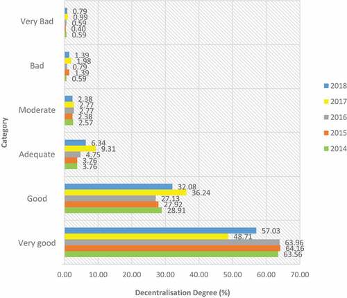
Figure 1 indicates that the horizontal axis is the decentralised degree ratio that measures the percentage of district original income to total district revenue. It indicates a region’s financial capabilities through its level of contribution of district/city revenue to county revenues. The higher the value of the decentralised degree ratio, the more the regional financial capability increases, implying that the financial contribution of the central government to the district/county is fewer. Sularso et al. (2011) concluded that one factor that indirectly affects economic growth is the ratio of degrees of decentralisation. Their results stated that the regional financial capability was almost 90 per cent, and the decentralisation process could be better, with 1 per cent being excellent, 1.5 per cent good, 2.5 per cent average, and 4 per cent sufficient. Overall, the last two years of findings (2017–2018) indicate an improvement in the decentralisation value ratio and regional financial capability.

Figure 1. Fiscal decentralisation in Indonesia; based on decentralisation degree 2014–2018.

Meanwhile, in Figure 2, the ratio of county financial independence is obtained from the distribution between district or city original income divided by the transfer income from the central and provincial governments and county loans. The increasing value of the county’s financial independence ratio means more regional financial independence.

Figure 2. Fiscal decentralisation in Indonesia: based on the Regional Independence Ratio 2014–2018.

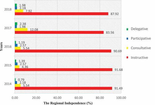
Results also indicate that the project distribution increased from 2014 to 2018 even though it did not significantly progress, likewise for qualitative indicators such as collaborative and instructive projects. Unfortunately, the instructive project still needs to be dominant from 2014 to 2018, achieving around 89 per cent of projects. As mentioned before, although fiscal decentralisation has been utilised for almost two decades, county financial capabilities are widely average, even slightly unsuccessful. One possible barrier is that the capacity of the public servant, economic structure, and political reforms of county government neither support budget efficiency nor facilitate an effective decision process. The fiscal decentralisation objective is to ease and effective policy decision-making, and finally, the regional product will increase the welfare of county citizens. However, the budgetary decentralisation effect on economic growth is still a fugue and debatable (Jin & Zau, 2005) (Bojanic, 2018), unequal economic growth of regions ((Martinez-Vazquez & McNab, 2003), relevant for the countries which are reforming the economic development (Yushkov, 2015). The empirical development of several regions varies. For example research by Ginting et al. (2019), showed that only Mimika and Surabaya City has high fiscal decentralization and high economic growth. Only a few district and City have high fiscal decentralization but low economic and the rest (91,3 per cent) have low fiscal decentralization and low economic growth. Therefore, to find out the outcome of a fiscal decentralisation policy on economic growth is not only to add the confidence level of the policymakers to continue and improve the procedure but also to provide strong academic support because the decentralisation of economic development that now becomes a mainstream issue in democratisation and systematic state area expansion in Indonesia. The current study examines the relationship between the transfer of control of a central government to local authorities and county financial independence. Similarly, Ginting et al. (2019) show that, on average, 91.3 per cent of districts/cities have relatively low fiscal decentralisation, with financial independence also being relatively low. According to Mahmudi (2010), some financial ratios can be made to analyse county financial capabilities, including the decentralisation degree ratio, county financial independence ratio, locally generated revenue effectiveness, and efficiency ratio.

Based on the abovementioned issue, most region or county independence (RI ratio) values are still low and have an instructive relationship pattern. Based on this exposure, the previous empirical research only looked at the influence of fiscal aspects on economic growth, so this study also looked at the impact of the Human Development Index (HDI). Several experts have also put forward the concept of human development; Sen (1989) defines human development as an extension of absolute freedom enjoyed by humans, where freedom depends on economic and social factors such as access to education, health, employment, and politics; put, a decent standard of living. Therefore, the study’s objective is to analyse the effects of fiscal decentralisation and human development on economic growth, relying on a standard framework of economic growth.

The remainder of the discussion of this study will be organised as follows. Section 2 briefly overviews the theoretical literature and empirical studies on financial decentralisation and county financial independence. Section 3 describes the investigation process and data used in the empirical analysis and model specifications, while Section 4 discusses the empirical results and findings. Finally, Section 5 concludes the study by summarising the findings, recommendations, and suggestions for future research.

2. Literature review

A significant feature of the current fiscal decentralisation literature is the need for more empirical information regarding the effects of decentralisation on economic growth and the traditional objectives of economic efficiency, income redistribution, and macroeconomic stability. As we subsequently discuss, the analysis of the direct role of the public sector in economic growth is a relatively new area of study, with the contribution of fiscal decentralisation to economic growth only emerging in the last decade. Consequently, we discuss i) theory and empirical evidence of a relationship between fiscal decentralisation and economic growth and ii) existing empirical evidence on the potential relationship between fiscal decentralisation and economic growth.

According to Shah (1998), the transfer of authority from central government into the local authority in regional autonomy, especially in developing countries, has used three types of decentralisation theory: politics, administrative and fiscal. Theoretically, several studies (Maryanov, 1965; Rondinelli, 1981; Smith, 1985; Mawhood, 1987; and Bird and Vaillancourt, 1998) have stated that the objectives of regional autonomy are distinguished into three main categories. The first is the purposes of the administration, including the creation of efficiency of the implementation of local government and the improvement of public services; the second is economic objectives, which aim to accelerate the process of economic development in the region to realise the welfare of the people; and the third is political purposes, which expedite the process of democratisation at the local, district, and city levels and the creation of public accountability.

In addition, fiscal decentralisation is defined as the devolution of fiscal powers from national to local governments. The principle behind federalisation is to improve efficiency in the provision and production of public goods, thereby enhancing and stimulating growth and development throughout the state. The theoretical underpinning of the effects of fiscal decentralisation on economic growth takes its legacy from the model of Tiebout and Tiebout (1956) and Oates (1972, 1999, 2005). However, as far as the empirical literature is concerned, there has yet to be a consensus on the relationship between the two, despite the attention it has received in the literature. Fiscal decentralisation can affect economic growth in different directions. Firstly, budgetary decentralisation can lead to economic growth due to public spending. Secondly, fiscal decentralisation might cause destabilisation of the economy, meaning a negative impact on economic growth. Thirdly, the effect of fiscal decentralisation on economic growth differs between developed and developing countries, specifically a positive impact in developed countries but a negative one in developing countries.

Fiscal decentralisation aims to increase the independence and capability of each region and improve the quality of human resources and the community’s welfare. Several previous studies, such as Akai and Sakata (2002), using a sample in the United States, found that fiscal decentralisation affected improving economic activities. On the other hand, Lin and Liu (2012) identified that budgetary decentralisation drives increased economic growth. Fiscal decentralisation is also expected to have a positive influence on public services, according to the extant literature (Adam et al., 2011; Faguet, 2008; Tiebout & Tiebout, 1956; Wang et al., 2012; Jia et al., 2014; Cavalieri and Ferrante, 2016, and Bodman et al., 2009). Reports have also described the nexus of fiscal decentralisation and economic growth in Oates (1993), who stated that decentralisation would create economic efficiency and have a dynamic effect on economic growth.

A comprehensive review of the studies is beyond the scope of this article. Within the context of the Solow—Swan model (Solow, 1956; Swan, 1956) of growth, fiscal federalism may be linked with a different level of efficiency in organisation and management than a centralised system, generating an additional value of total factor productivity (Solow’s A) or the level of technology. Therefore, with decentralisation, countries will witness variations in their growth rates. The innovation process will get triggered efficiently in a federal system (Feld et al., 2012).

While several recent studies have attempted to quantify the role of government expenditures on economic growth, Aschauer (1989) and Barro (1990) ascertained that an increasing share of central government consumption in GDP is negatively associated with an increase in per capita income. Besides this, Gifari (2016) examined the impact of government expenditure on economic growth and utilised the Ordinary Least Square (OLS) technique with time series data from 1970 to 2014 in Malaysia. They found a negative correlation between government expenditure and economic growth. However, in an earlier study, Ram (1986) discovered that central government consumption positively influences GDP and growth in per capita income.

None of the studies previously mentioned is concerned with the potential impact of the degree of fiscal decentralisation on economic growth. An emerging line of research has attempted to test the presence of a direct link between fiscal decentralisation and economic development with mixed results. The standard measures of fiscal decentralisation utilised in most decentralisation studies are the total subnational government revenues to general government revenues and total subnational government expenditures to general government expenditures (Bojanic, 2018). However, some researchers measured fiscal decentralisation differently; expenditure-based decentralisation (ED), revenue-based decentralisation (RD), and tax revenue-based decentralisation (TRD) (Hung & Thanh, 2022), the ratio of own revenues/expenditures to general government revenues/expenditure (Wang et al., 2021), decentralisation of income and expenditure (Burret et al., 2021), decentralisation indicators (fiscal, administrative, and political (Bojanic & Collins, 2021), the share of village government budget that came from revenue transfer from the central government (Pal & Wahhaj, 2017), the ratio of per capita provincial budgetary expenditures to the sum of per capita central budgetary expenditures and local budgetary expenditures (Brock et al., 2015), we can conclude that fiscal decentralisation is the intergovernmental composition of public expenditure or revenue assignment (Martinez-Vasquez & McNab, 2003).

Although the empirical findings on the link are mixed, they heavily lean to the positive side; many studies have validated that fiscal decentralisation is desirable and exerts a positive impact on fiscal, social, and economic indicators. Indeed, Thiessen (2000) found a positive and direct relationship between decentralisation and economic growth for panels of high-income, Western European, and middle-income countries. Likewise, Gemmell et al. (2013) and Martinez-Vazquez et al. (2017) found strong evidence that fiscal decentralisation positively correlates with economic growth once the endogeneity issue is controlled. These results support earlier studies that also report a positive connectedness between fiscal decentralisation and economic growth. In Addition, Permai et al. (2021) examined the effect of fiscal decentralisation on regional financial performance with the Geographically Weighted Regression (GWR) method on Sumatra Island, Indonesia. Based on the GWR model results, all independent variables significantly and positively affected economic performance.

In contrast, Yushkov (2015) investigated the relationship between fiscal decentralisation and economic growth with an empirical analysis of Russian regions from 2005 to 2012, showing that excessive expenditure decentralisation within the region, which is not accompanied by the respective level of revenue decentralisation, is significantly and negatively related to regional economic growth. Bojanic (2018) analysed the impact of fiscal decentralisation on economic growth, inflation, and Gini coefficients in 12 countries in the Americas. The findings suggest that the positive effects of this process have been more modest than anticipated, with revenue decentralisation having a detrimental impact on economic growth and expenditure decentralisation a positive one in developing nations. Also, Nguyen et al. (2022) found that fiscal decentralisation on economic growth, economic growth does not give rise to the efficiency of fiscal decentralisation yet could reduce human development instead. The results provide several plausible implications for policymakers.

In the same vein, Jin and Rider (2020) examined the effect of fiscal decentralisation on short- and long-run economic growth and estimated two-step generalised method of moment (GMM) simultaneous equations models, using panel data for China and India for the period 1985 to 2005. As a result, they concluded that fiscal decentralisation has a negative and statistically significant effect at conventional levels on short-run economic growth for both China and India. Nevertheless, Thornton (2007) failed to find a statistically significant relationship between fiscal decentralisation and economic growth for 19 OECD member countries. The relationship between fiscal decentralisation and economic growth might be best characterised as inconclusive.

On the other hand, Hao et al. (2021) used the panel data of 23 Chinese provinces between 2002 and 2012 and used the simultaneous equation model to control for potential endogeneity. The results indicate that higher income inequality significantly negatively impacts public health performance. Interestingly, fiscal decentralisation has adverse direct and indirect effects on public health. Then Bojanic and Collins (2021) applied a panel data set of OECD and non-OECD countries from 1980 to 2016; unlike prior literature, they examine the effects of fiscal, administrative, and political decentralisation on inequality both individually and in interaction. They find that decentralisation reduces income inequality, but the effect diminishes and eventually reverses as economic development increases. These findings imply that the overall decentralisation mix is vital for income inequality, and both a country’s current stage in development and underlying institutional framework should be considered when determining the decentralisation mix.

A discussion of fiscal decentralisation and financial independency is still in progress. This concerns large developing countries, especially those with restructuring economic reforms. Finding the best practice of practical experience remains challenging and an opportunity for researchers. Based on the findings, exploring this issue is still contributing to policymakers and improving the existing theory related to fiscal decentralisation, human development, and financial independence in regional economic development.

3. Methods

This paper aims to analyse the effects of fiscal decentralisation and the HDI on economic growth, relying on a standard framework of economic growth. This paper employs the form’s Cobb-Douglas production function (Mankiw et al., 1992).

(1) $y(t)\hspace{0.17em}=A(t)K(t{)}^{\alpha }{L}^{1-\alpha }$(1)

Y is GDP, k is capital, A is the level of technology, and L is labour, which is assumed to be constant. Equation 1(1) $y(t)\hspace{0.17em}=A(t)K(t{)}^{\alpha }{L}^{1-\alpha }$(1) is converted into a growth equation so that the economic growth follows a process expressed in the following equation:

(2) $g(t)\hspace{0.17em}=y(t)\hspace{0.17em}=A(t)\hspace{0.17em}+\alpha k(t)$(2)

According to Equation 2(2) $g(t)\hspace{0.17em}=y(t)\hspace{0.17em}=A(t)\hspace{0.17em}+\alpha k(t)$(2) , economic growth depends on technology and capital. According to Lin and Liu (2012), the increase in technology comes from technological changes and differences in natural resources and regional developments.

Based on Equation 1(1) $y(t)\hspace{0.17em}=A(t)K(t{)}^{\alpha }{L}^{1-\alpha }$(1) and Equation 2(2) $g(t)\hspace{0.17em}=y(t)\hspace{0.17em}=A(t)\hspace{0.17em}+\alpha k(t)$(2) , also inspired by Lin and Liu (2012), we relaxed the labour assumption is constant because we argue that after several years the human capital development should increase because the schooling period of each level will take an average of around six-year for primary school to high school and 4-year from high school to undergraduate level. Yushkov (2015) argued that a Cobb-Douglas production has two inputs, namely private capital, and public spending, by three levels of government federal, state and local. Public expenditures are financed through taxes on output. Maximising the utility function of a representative agent for a dynamic budget constraint provides the following solution: output growth rate depends, among other things, on the shares of different levels of government in total public expenditure. In addition, then fiscal decentralisation is a change of differences in capital resources allocation of regions; also, fiscal decentralisation implies technological changes, the decision process of allocating and managing economic resources.

3.1. Variable measurements and data sources

The study of the regional development model is the function of fiscal decentralisation and human development. The unit analysis of the study is 484 regions or counties (districts or cities) from 34 provinces in Indonesia, and the period investigated is from 2014 to 2019. The source of data is the Indonesian Ministry of Finance (MOF).

The fiscal decentralisation variables consist of the growth of degree decentralisation (DD), a general term for transferring powers and resources from higher to lower levels in a political system. This is measured using locally generated revenue divided by total county revenue. The central government grants (GG) are the balancing funds sourced from central government budget revenues allocated to (autonomous) regions to fund regional needs in implementing decentralisation. The measurement of GG balances funds divided by one billion Rupiah as maximum funds. The balance fund amount is determined every fiscal year in the government budget. The region independence variable is the region or county independence (RI), which is the ability of regions to finance local government expenditure and is represented in the budget. This is measured through locally generated revenue divided by the transfer and assistance from the central government, provincial government, and regional loans. The transfer and assistance from the central government, provincial government, and regional loans (TL) are the total funds consisting of the transfer income from the central and provincial governments and regional loans. Human resources development is the growth of the HDI, which is the social and economic development level. It comprises three principal areas of interest: 1) health fields, longevity, namely life expectancy at birth; 2) education fields, knowledge consisting of the mean years of schooling, expected years of education; and 3) Economic fields, decent living. Growth of Gross Regional Domestic Product (GRDP) is the gross added value of all goods and services produced in the domestic territory arising from various economic activities. This value is usually within a certain period regardless of whether the factors of production are resident or non-resident.

3.2. Specification model

As the consequences of the data type are a combination of time series and cross-sections, we utilise the panel data analysis method. Panel data combining cross-section and time series allow us to control variables that cannot be observed or measured, like country factors, companies, and time variation. This accounts for individual and time heterogeneity. With panel data, we can include variables at different analysis levels suitable for multilevel or hierarchical modelling. At the same time, the trend of the data can be analysed. Model estimation started with static panel data methods such as pooled data, fixed effect model (FEM) and random effect model (REM). Where pooled data analysis is assumed to be constant, and the slope of the regression equation is fixed whether individual or time varies, it is not appropriate for panel data due to many individual and time variances.

Second, the model estimation is also examined using dynamic panel data methods since the rationale of economic development will be influenced by previous economic growth. In this matter, there are two models: first, different GMM (DGMM) and system GMM (SGMM).

This study aimed to explore the effect of fiscal decentralisation policies and human capital development on regional domestic product growth. The research model will subsequently present the impact of these factors on the growth of the regional domestic product.

3.3. Static panel data analysis

Fiscal decentralisation as a part of capital resources allocation of regions and technological changes and human capital development will affect regional economic growth (Mankiw et al., 1992; Lin and Liu (2012). Then, we measured the fiscal decentralisation through some indicators or measurements such as the transfer of authority from central to local government through the DD, regional independence (RI), GG, transfer and assistance from the central government, provincial government, and county loans (TL), and the growth of HDI as presented human capital development. Since the study uses panel data, Equation 1(1) $y(t)\hspace{0.17em}=A(t)K(t{)}^{\alpha }{L}^{1-\alpha }$(1) can be rewritten as follows, and the data can be transformed into a natural log:

(3) $\mathrm{L}\mathrm{G}\mathrm{R}\mathrm{D}{\mathrm{P}}_{\mathrm{i},\mathrm{t}}={\beta }_{\mathrm{o}}+{\beta }_1\mathrm{L}\mathrm{D}{\mathrm{D}}_{\mathrm{i},\mathrm{t}}+{\beta }_2\mathrm{L}\mathrm{G}{\mathrm{G}}_{\mathrm{i},\mathrm{t}}+{\beta }_3\mathrm{L}\mathrm{R}{\mathrm{I}}_{\mathrm{i},\mathrm{t}}+{\beta }_4\mathrm{L}\mathrm{T}{\mathrm{L}}_{\mathrm{i},\mathrm{t}}+{\beta }_5\mathrm{L}\mathrm{H}{\mathrm{D}}_{\mathrm{i},\mathrm{t}}+{\alpha }_{\mathrm{i},\mathrm{t}}$(3)

Where α_i,t is the term error, i is a cross-section, county 1 to n, t is the period, time 1 to t, and L represents the log number.

Based on Equation 3(3) $\mathrm{L}\mathrm{G}\mathrm{R}\mathrm{D}{\mathrm{P}}_{\mathrm{i},\mathrm{t}}={\beta }_{\mathrm{o}}+{\beta }_1\mathrm{L}\mathrm{D}{\mathrm{D}}_{\mathrm{i},\mathrm{t}}+{\beta }_2\mathrm{L}\mathrm{G}{\mathrm{G}}_{\mathrm{i},\mathrm{t}}+{\beta }_3\mathrm{L}\mathrm{R}{\mathrm{I}}_{\mathrm{i},\mathrm{t}}+{\beta }_4\mathrm{L}\mathrm{T}{\mathrm{L}}_{\mathrm{i},\mathrm{t}}+{\beta }_5\mathrm{L}\mathrm{H}{\mathrm{D}}_{\mathrm{i},\mathrm{t}}+{\alpha }_{\mathrm{i},\mathrm{t}}$(3) , the fiscal decentralisation and HDI’s influence on the growth of regional domestic products is estimated:

(4) $\mathrm{L}\mathrm{G}\mathrm{R}\mathrm{D}{\mathrm{P}}_{\mathrm{i},\mathrm{t}}={\beta }_{\mathrm{o}\mathrm{i}}+{\beta }_1\mathrm{L}\mathrm{D}{\mathrm{D}}_{\mathrm{i},\mathrm{t}}+{\beta }_2\mathrm{L}\mathrm{G}{\mathrm{G}}_{\mathrm{i},\mathrm{t}}+{\beta }_3\mathrm{L}\mathrm{R}{\mathrm{I}}_{\mathrm{i},\mathrm{t}}+{\beta }_4\mathrm{L}\mathrm{T}{\mathrm{L}}_{\mathrm{i},\mathrm{t}}+{\beta }_5\mathrm{L}\mathrm{H}{\mathrm{D}}_{\mathrm{i},\mathrm{t}}+{\alpha }_{\mathrm{i},\mathrm{t}}$(4)

Although constant, the term fixed effect from Equation 4(4) $\mathrm{L}\mathrm{G}\mathrm{R}\mathrm{D}{\mathrm{P}}_{\mathrm{i},\mathrm{t}}={\beta }_{\mathrm{o}\mathrm{i}}+{\beta }_1\mathrm{L}\mathrm{D}{\mathrm{D}}_{\mathrm{i},\mathrm{t}}+{\beta }_2\mathrm{L}\mathrm{G}{\mathrm{G}}_{\mathrm{i},\mathrm{t}}+{\beta }_3\mathrm{L}\mathrm{R}{\mathrm{I}}_{\mathrm{i},\mathrm{t}}+{\beta }_4\mathrm{L}\mathrm{T}{\mathrm{L}}_{\mathrm{i},\mathrm{t}}+{\beta }_5\mathrm{L}\mathrm{H}{\mathrm{D}}_{\mathrm{i},\mathrm{t}}+{\alpha }_{\mathrm{i},\mathrm{t}}$(4) can be different for individual banks, and it will not remain constant for an extended period, known as “time-invariant”. A random effect analysis is evidenced in base Equation 4(4) $\mathrm{L}\mathrm{G}\mathrm{R}\mathrm{D}{\mathrm{P}}_{\mathrm{i},\mathrm{t}}={\beta }_{\mathrm{o}\mathrm{i}}+{\beta }_1\mathrm{L}\mathrm{D}{\mathrm{D}}_{\mathrm{i},\mathrm{t}}+{\beta }_2\mathrm{L}\mathrm{G}{\mathrm{G}}_{\mathrm{i},\mathrm{t}}+{\beta }_3\mathrm{L}\mathrm{R}{\mathrm{I}}_{\mathrm{i},\mathrm{t}}+{\beta }_4\mathrm{L}\mathrm{T}{\mathrm{L}}_{\mathrm{i},\mathrm{t}}+{\beta }_5\mathrm{L}\mathrm{H}{\mathrm{D}}_{\mathrm{i},\mathrm{t}}+{\alpha }_{\mathrm{i},\mathrm{t}}$(4) . Even though Equation 4(4) $\mathrm{L}\mathrm{G}\mathrm{R}\mathrm{D}{\mathrm{P}}_{\mathrm{i},\mathrm{t}}={\beta }_{\mathrm{o}\mathrm{i}}+{\beta }_1\mathrm{L}\mathrm{D}{\mathrm{D}}_{\mathrm{i},\mathrm{t}}+{\beta }_2\mathrm{L}\mathrm{G}{\mathrm{G}}_{\mathrm{i},\mathrm{t}}+{\beta }_3\mathrm{L}\mathrm{R}{\mathrm{I}}_{\mathrm{i},\mathrm{t}}+{\beta }_4\mathrm{L}\mathrm{T}{\mathrm{L}}_{\mathrm{i},\mathrm{t}}+{\beta }_5\mathrm{L}\mathrm{H}{\mathrm{D}}_{\mathrm{i},\mathrm{t}}+{\alpha }_{\mathrm{i},\mathrm{t}}$(4) stated that β_oi is fixed, we assumed it is a random variable with an average value, βo. Constant could be written as:

(5) ${\beta }_{0\mathrm{i}}={\beta }_0+{\mathrm{e}}_{\mathrm{i}}\mathrm{i}=1,2,...........,\mathrm{N}$(5)

Where ε_i is the error term with an average value of zero and variance σ². It replaces Equation 4(4) $\mathrm{L}\mathrm{G}\mathrm{R}\mathrm{D}{\mathrm{P}}_{\mathrm{i},\mathrm{t}}={\beta }_{\mathrm{o}\mathrm{i}}+{\beta }_1\mathrm{L}\mathrm{D}{\mathrm{D}}_{\mathrm{i},\mathrm{t}}+{\beta }_2\mathrm{L}\mathrm{G}{\mathrm{G}}_{\mathrm{i},\mathrm{t}}+{\beta }_3\mathrm{L}\mathrm{R}{\mathrm{I}}_{\mathrm{i},\mathrm{t}}+{\beta }_4\mathrm{L}\mathrm{T}{\mathrm{L}}_{\mathrm{i},\mathrm{t}}+{\beta }_5\mathrm{L}\mathrm{H}{\mathrm{D}}_{\mathrm{i},\mathrm{t}}+{\alpha }_{\mathrm{i},\mathrm{t}}$(4) and Equation 5(5) ${\beta }_{0\mathrm{i}}={\beta }_0+{\mathrm{e}}_{\mathrm{i}}\mathrm{i}=1,2,...........,\mathrm{N}$(5) , so the equation is:

(6) $\mathrm{L}\mathrm{G}\mathrm{R}\mathrm{D}{\mathrm{P}}_{\mathrm{i},\mathrm{t}}={\beta }_{\mathrm{o}\mathrm{i}}+{\beta }_1\mathrm{L}\mathrm{D}{\mathrm{D}}_{\mathrm{i},\mathrm{t}}+{\beta }_2\mathrm{L}\mathrm{G}{\mathrm{G}}_{\mathrm{i},\mathrm{t}}+{\beta }_3\mathrm{L}\mathrm{R}{\mathrm{I}}_{\mathrm{i},\mathrm{t}}+{\beta }_4\mathrm{L}\mathrm{T}{\mathrm{L}}_{\mathrm{i},\mathrm{t}}+{\beta }_5\mathrm{L}\mathrm{H}{\mathrm{D}}_{\mathrm{i},\mathrm{t}}+{\alpha }_{\mathrm{i},\mathrm{t}}$(6)

(7) ${\omega }_{\mathrm{i}\mathrm{t}}={\epsilon }_{\mathrm{i}}+{\mathrm{u}}_{\mathrm{i}\mathrm{t}}$(7)

Where the error term composite ω_it consists of two components, ε_i is the error for the cross-sectional component, and Equation 7(7) ${\omega }_{\mathrm{i}\mathrm{t}}={\epsilon }_{\mathrm{i}}+{\mathrm{u}}_{\mathrm{i}\mathrm{t}}$(7) is an error in the combination component of time series and crossnational.

Random and fixed effects investigate whether the model followed random or fixed effects by applying the Hausman test. The null hypothesis is a random effect (individual effect uncorrelated), and the alternate hypothesis is a fixed effect. The statistical test ${\chi }_{hit}^2=(b-\beta {)}^{\prime }Var(b-\beta {)}^{-1}(b-\beta )$ shows that b is the coefficient for random effect and β is the coefficient for fixed effect. The null hypothesis is rejected if ${\chi }_{hit}^2\succ {\chi }_{(k,\alpha )}$. Next, we select models to choose the best estimate by conducting the chow, Hausman, and LM tests. After obtaining the best model to estimate, the theory sign, significance test, goodness of fit test, coefficient of determination test, and F test are conducted.

3.4. Dynamic panel data analysis

The basic model of the dynamic panel data model is:

(8) $y_{it}={\rho }_i{y}_{it-1}+z_{it}\gamma +c_i+u_{it}$(8)

Where u_it is the error with a mean of zero and a fixed variance, z_it is a matrix of exogenous variables, and y_it-1 is a predetermined variable (exogenous variables are derived from endogenous variables).

According to Arellano and Bond (1991), the solutions of dynamic panel data model AR (1) and a 2SLS (two-stage least squares) estimation can produce consistent results. However, they may not be efficient (no minimum variance). Therefore, we do not consider that a conditioning moment exists. Arellano and Bond suggest using Δy_it-2 as instruments of Δy_it-1. This procedure results in a more efficient procedural estimator (Aderson & Hsiao, 1998). Therefore, following Arellano and Bond, we use an estimator with GMM (general method of moments) to estimate ${\alpha }_1\dots .{\alpha }_{\rho },{\beta }_1,{\beta }_2$.

(9) $y_{it}=y_{it-1}{\alpha }_1+\dots +y_{it-\rho }{\alpha }_{\rho }+x_{it}{\beta }_1+z_{it}{\beta }_2+c_i+u_{it}$(9)

Where x_it is a strictly exogenous variable (matrix), z_it is a predetermined variable matrix), c_i is random effects, iid means independent and identically distributed, and u_it is an error term, iid.

Equation 9(9) $y_{it}=y_{it-1}{\alpha }_1+\dots +y_{it-\rho }{\alpha }_{\rho }+x_{it}{\beta }_1+z_{it}{\beta }_2+c_i+u_{it}$(9) is transformed into the actual research variable (Equation 3(3) $\mathrm{L}\mathrm{G}\mathrm{R}\mathrm{D}{\mathrm{P}}_{\mathrm{i},\mathrm{t}}={\beta }_{\mathrm{o}}+{\beta }_1\mathrm{L}\mathrm{D}{\mathrm{D}}_{\mathrm{i},\mathrm{t}}+{\beta }_2\mathrm{L}\mathrm{G}{\mathrm{G}}_{\mathrm{i},\mathrm{t}}+{\beta }_3\mathrm{L}\mathrm{R}{\mathrm{I}}_{\mathrm{i},\mathrm{t}}+{\beta }_4\mathrm{L}\mathrm{T}{\mathrm{L}}_{\mathrm{i},\mathrm{t}}+{\beta }_5\mathrm{L}\mathrm{H}{\mathrm{D}}_{\mathrm{i},\mathrm{t}}+{\alpha }_{\mathrm{i},\mathrm{t}}$(3) ) to explore the effect of fiscal decentralisation and human development on the growth of RDP. The dynamic panel data process of the dependent variable is:

(10) $\mathrm{L}\mathrm{G}\mathrm{R}\mathrm{D}{\mathrm{P}}_{\mathrm{i}\mathrm{t}}={\beta }_0+{\beta }_1\mathrm{L}\mathrm{G}\mathrm{R}\mathrm{D}\mathrm{P}\mathrm{i}{\mathrm{t}}_{-1}+{\beta }_2\mathrm{L}\mathrm{D}{\mathrm{D}}_{\mathrm{i}\mathrm{t}}+{\beta }_3\mathrm{L}\mathrm{G}{\mathrm{G}}_{\mathrm{i}\mathrm{t}}+{\beta }_4\mathrm{L}\mathrm{R}{\mathrm{I}}_{\mathrm{i}\mathrm{t}}+{\beta }_5\mathrm{L}\mathrm{T}{\mathrm{L}}_{\mathrm{i}\mathrm{t}}+{\beta }_6\mathrm{L}\mathrm{H}{\mathrm{D}}_{\mathrm{i}\mathrm{t}}+{\omega }_{\mathrm{i}\mathrm{t}}$(10)

(11) $\hspace{0.17em}{\omega }_{\mathrm{i}\mathrm{t}}={\epsilon }_{\mathrm{i}}+{\mathrm{u}}_{\mathrm{i}\mathrm{t}}$(11)

Equation 10(10) $\mathrm{L}\mathrm{G}\mathrm{R}\mathrm{D}{\mathrm{P}}_{\mathrm{i}\mathrm{t}}={\beta }_0+{\beta }_1\mathrm{L}\mathrm{G}\mathrm{R}\mathrm{D}\mathrm{P}\mathrm{i}{\mathrm{t}}_{-1}+{\beta }_2\mathrm{L}\mathrm{D}{\mathrm{D}}_{\mathrm{i}\mathrm{t}}+{\beta }_3\mathrm{L}\mathrm{G}{\mathrm{G}}_{\mathrm{i}\mathrm{t}}+{\beta }_4\mathrm{L}\mathrm{R}{\mathrm{I}}_{\mathrm{i}\mathrm{t}}+{\beta }_5\mathrm{L}\mathrm{T}{\mathrm{L}}_{\mathrm{i}\mathrm{t}}+{\beta }_6\mathrm{L}\mathrm{H}{\mathrm{D}}_{\mathrm{i}\mathrm{t}}+{\omega }_{\mathrm{i}\mathrm{t}}$(10) has some potential technical problems. First, there is causality between independent variables and the possibility of regressors related to the error term. The best solution to the problem is using the first difference, GMM, as suggested by Arellano and Bond 1991. Equation 10(10) $\mathrm{L}\mathrm{G}\mathrm{R}\mathrm{D}{\mathrm{P}}_{\mathrm{i}\mathrm{t}}={\beta }_0+{\beta }_1\mathrm{L}\mathrm{G}\mathrm{R}\mathrm{D}\mathrm{P}\mathrm{i}{\mathrm{t}}_{-1}+{\beta }_2\mathrm{L}\mathrm{D}{\mathrm{D}}_{\mathrm{i}\mathrm{t}}+{\beta }_3\mathrm{L}\mathrm{G}{\mathrm{G}}_{\mathrm{i}\mathrm{t}}+{\beta }_4\mathrm{L}\mathrm{R}{\mathrm{I}}_{\mathrm{i}\mathrm{t}}+{\beta }_5\mathrm{L}\mathrm{T}{\mathrm{L}}_{\mathrm{i}\mathrm{t}}+{\beta }_6\mathrm{L}\mathrm{H}{\mathrm{D}}_{\mathrm{i}\mathrm{t}}+{\omega }_{\mathrm{i}\mathrm{t}}$(10) is thus transformed into the first-difference form:

(12) $\mathrm{\Delta }\mathrm{L}\mathrm{G}\mathrm{R}\mathrm{D}{\mathrm{P}}_{\mathrm{i}\mathrm{t}}={\beta }_0+{\beta }_1\mathrm{\Delta }\mathrm{L}\mathrm{G}\mathrm{R}\mathrm{D}{\mathrm{P}}_{\mathrm{i}\mathrm{t}-1}+{\beta }_2\mathrm{\Delta }\mathrm{L}\mathrm{D}{\mathrm{D}}_{\mathrm{i}\mathrm{t}}+{\beta }_3\mathrm{\Delta }\mathrm{L}\mathrm{G}{\mathrm{G}}_{\mathrm{i}\mathrm{t}}+{\beta }_4\mathrm{\Delta }\mathrm{L}\mathrm{R}{\mathrm{I}}_{\mathrm{i}\mathrm{t}}+{\beta }_5\mathrm{\Delta }\mathrm{L}\mathrm{T}\mathrm{P}{\mathrm{L}}_{\mathrm{i}\mathrm{t}}+{\beta }_6\mathrm{\Delta }\mathrm{L}\mathrm{H}{\mathrm{D}}_{\mathrm{i}\mathrm{t}}+\mathrm{\Delta }{\omega }_{\mathrm{i}\mathrm{t}}$(12)

In its general form, the transformation is given as ∆LGRDP_it = β₀ + β₁∆LGRDP_it-1 + β₂∆LDD_it + β₃∆LGG_it + β₄∆LRI_it + β₅∆LTPL_it + β₆∆LHD_it + ∆ω_it by transforming the regressors by first difference, and the fixed-county effect is removed, because time is not invariant. From Equation 13(13) $\mathrm{\Delta }{\omega }_{\mathrm{i}\mathrm{t}}=\mathrm{\Delta }{\epsilon }_{\mathrm{i}}+\mathrm{\Delta }{\mathrm{u}}_{\mathrm{i}\mathrm{t}}$(13) , we obtain:

(13) $\mathrm{\Delta }{\omega }_{\mathrm{i}\mathrm{t}}=\mathrm{\Delta }{\epsilon }_{\mathrm{i}}+\mathrm{\Delta }{\mathrm{u}}_{\mathrm{i}\mathrm{t}}$(13)

Arellano and Bover (1995) suggest a new estimation process to improve Arellano and Bond 1991 in which there is an exogenous variable that is endogenous to the right side of the equation (or, in other words, there is a correlation with the number of exogenous variable error terms). Unlike Arellano and Bond 1991, Arellano and Bover (1995) did not perform the first-difference transformation but instead used the transformation (separation of variables, the right side of the equation of a purely exogenous endogenous and exogenous nature) such that orthogonal conditions are met. This estimator and the use of GMM also apply 3SLS (three-stage least squares) to estimate the instrumental variable.

4. Finding and discussion

The data analysis is based on three models. In Model (1), the analysis is based on the overall sample of 484 regions or countries (districts and cities). In Model (2), the study against the district or cities with county independence is below 50 per cent. In Model (3), the analysis against the county with county independence is above 50 per cent. Based on the robustness test results for the three estimates in this study, the best model is the FEM and SGMM based on the robustness test.

This study utilised fiscal decentralisation and the HDI, which can influence RDP growth in all counties. The theory used in this study shows that the five variables positively influence the growth of RDP in Indonesia. Data processing is carried out using multiple linear regression.

Based on Table 1, we show the results of the static panel data analysis. The results for the RDP growth Model 1 to Model 3 found that the Chow test shows the probability value of a Cross-section Chi-Square of 0.0000 < 0.05 (alpha 5 per cent). The null hypothesis was rejected, so we conducted the Hausman test with a probability value of Cross Section Random of 0.0000 < 0.05 (alpha 5 per cent), thus, Ho was rejected. The best model to estimate RDP growth is the fixed-effect model (FEM). The estimates produced from Model 1 GRDP for all regions/cities in Indonesia during 2014–2019 are subsequently explained.

Table 1. Result of static panel data analysis. Dependent Variable: Growth of Regional Domestic Product (LGRDP)

Independent Variables	FIXED EFFECT
	Model 1	MODEL 2	MODEL 3
LDD	−0.2113*** (0.0000)	−0.1926*** (0.0000)	0.03557* (0.0883)
LGG	0.1146*** (0.0000)	0.1188*** (0.0000)	0.0204 (0.3821)
LORI	0.2272*** (0.0000)	0.2085*** (0.0000)	0.0799*** (0.0002)
LTL	−0.0022 (0.8911)	−0.0097 (0.6417)	0.1952*** (0.0000)
LHD	4.0814*** (0.0000)	4.0829*** (00.0000)	5.4587*** (0.0000)
Constant	5.0536*** (0.0000)	5.0243*** (0.0000)	−0.8870 (0.4491)
The goodness of the Fit Model
R-square	0.9989	0.9987	0.9994
F test	5338.52*** (0.0000)	4633.01*** (0.0000)	8402.74*** (0.0000)
Model Selection Test
Chow Test (Chi-square)	5928.39 (0.0000)	5596.01 (0.0000)	733.01 (0.0000)
Hausman test	106.69 (0.0000)	84.71 (0.0000)	41.34 (0.0000)
NxT	2904	2904	2904

The parenthesis are probabilities, except for the F (Walt) test, BP-LM test,

Hausman test, F test, are p-values. *** p ≤ 1%, ** p ≤ 5% and * p ≤ 1%

In addition, the findings stated that the determination of GRDP Models 1 to 3 is 99.88 per cent, 99.87, per cent and 99.94 per cent, respectively, each at the significance level of 1 per cent. This means that independent variables explain GRDP of 99.88 per cent at a significance level of 1 per cent, while other independent variables are not included in the model.

Model 1 showed that of the five independent variables used in this study of GRDP, two variables do not follow the theory proposed in this study, namely the LDD and LTL. The negative coefficients mean that the higher the LDD and LTL, the lower the GRDP, so it is concluded in this study that both variables reduce the growth of RDP. The other three variables produce a positive coefficient of GRDP, meaning that the higher the county independence (LRI), the GG, and the HDI, the higher the GRDP. The unsatisfied result of degree decentralisation and the transfer of income from the central and provincial governments and regional loans might be due to the fiscal decentralisation being too young, even though enacted since the year 1999. However, the government still emends until the year 2015. In addition, strong economic and political institutions are needed to support the reform process, implying an incomplete decentralisation ecosystem.

Model 2 showed that of the five variables used in this study to see factors that affect the growth of GRDP, two variables do not correspond to the theory proposed in this study, namely the LDD and LTL. The sign is a negative coefficient, meaning that the higher the LDD and LTL, the lower the GRDP, so it is concluded in this study that both variables reduce the GRDP. The other three variables produce a positive coefficient of GRDP growth, meaning that the higher the growth of county independence (LRI), the GG, and the growth of the human development index (LHD), the higher the GRDP.

Model 3 used five variables in this study to see the factors that affect the GRDP. The LGG is insignificant but follows the theory proposed in this study, namely the GG, meaning that the increase in GG cannot increase RDP’s growth in counties with high county independence or those above 50 per cent. The other four variables are LDD, LRI, TL, and LHD, producing a positive coefficient and significant RDP growth, meaning that the higher the four variables, the higher the GRDP.

Table 2 shows the result of a dynamic panel data analysis, DGMM, and SGMM analysis concerning Equation 13(13) $\mathrm{\Delta }{\omega }_{\mathrm{i}\mathrm{t}}=\mathrm{\Delta }{\epsilon }_{\mathrm{i}}+\mathrm{\Delta }{\mathrm{u}}_{\mathrm{i}\mathrm{t}}$(13) Every model was analysed using one-step and two-step in the growth of Models 1 to 3. This part focuses on whether fiscal decentralisation encourages the county to make more independent decisions and is suitable for local problems. The overidentifying restrictions test or the Sargant test shows that the null hypothesis cannot be rejected at a significant 5 per cent level, and there is no serial correlation, as shown by the fact that AR(1) is significant and AR(2) is insignificant. Therefore, both models (DGMM and SGMM) are valid for two steps, but SGMM gives better results because the coefficient of lag GRDP is higher than DGMM, except that Model 1 is the opposite of the lower and the upper bounds.

Table 2. Result of dynamic panel data analysis. Dependent Variable: Growth of Regional Domestic Product (LGRDP)

	Model 1		Model 2		Model 3
	DGMM (Two-step)	SGM (Two-step)	DGMM (Two-step)	SGM (Two-step)	DGMM (Two-step)	SGM (Two-step)
Constant	4.940*** (2.3525)	4.114** (2.1821)	3.043 (2.464)	1.9063 (2.089)	−7.1994 (4.8108)	12.748*** (2.0193)
Lag LGRDP	0.472*** (0.0536)	0.450*** (0.0316)	0.536*** (0.040)	0.551*** (0.0263)	−0.063*** (0.0199)	0.170*** (0.0377)
LDD	0.064*** (0.0230)	0.088** (0.0463)	0.161*** (0.0614)	0.163*** (0.0616)	−0.0128 (0.01784)	−0.066*** (0.0317)
LGG	0.0008*** (0.0004)	0.001*** (0.0003)	0.0009*** (0.0004)	0.0008** (0.0004)	0.0001 (0.0002)	0.0007*** (0.0001)
LORI	−0.025*** (0.0089)	−0.0458 (0.0309)	−0.094*** (0.0430)	−0.098*** (0.0428)	−0.0022 (0.0031)	0.027*** (0.0089)
LTPL	−0.0004 (0.0004)	−0.0005 (0.0003)	−0.0006 (0.0004)	−0.0007* (0.0004)	−0.001*** (0.0002)	0.0001 (0.0002)
LHD	−0.0409 (0.0400)	−0.0248 (0.0367)	−0.0169 (0.0416)	0.0012 (0.0360)	0.192*** (0.0633)	−0.112*** (0.0203)
Sargent test	16.81057*	21.7645*	16.6838*	19.6911	7.7846	14.9319
AR(1)	−2.894***	−2.960***	−3.125***	−3.17***	−2.104***	−2.163***
AR(2)	1.0886	1.0856	0.85624	0.83903	−1.1805	−0.35825
NxT	2000	2500	1920	2400	76	95

Standard errors are in parentheses; statistical significance: *** p ≤ 1%, ** p ≤ 5%,

and * p ≤ 10%. NxT is the total sample (cross-section multiplied by time series).

The result indicated that, based on SGMM’s two-step analysis, the first difference between GRDP, LDD, and LGG positively affects the GRDP at a significance level of 1 per cent, except it negatively affected LDD for Model 3, which has a significant level of 5 per cent. The other variables, such as LRI, LTL, and LHD, harm GRDP. However, LRI and LTL positively impact GRDP in Model 3 and LHD in Model 2. Where the effect of LRI is negative and significant at the 1 per cent level, LTL has a negative impact at the significance level of 10 per cent in Model 2 only, and LHD has a negative effect and significance level of 1 per cent in Model 3. The result implies that an increase in the LDD and LGG will increase the GRDP, increase the LRI, and decrease RDP growth. LTL and LHD are insignificant to GRDP in the overall sample.

This finding is exciting, as it implies that fiscal decentralisation policies and HDI can cause growth in county development. The increase in GG and decentralisation subsequently increase regional domestic product growth. When a region has budgetary decentralisation, a policymaker can understand the real problems and needs of the public and private institutions and their people; therefore, allocating economic resources is effective and efficient and increases productivity.

We use a basic validity model across three models. The model shows that a one-step result for both DGMM and SGMM is rejected because the null hypothesis is not rejected in the Sargan test, where a probability higher than chi-square is 0.000 for both models. The auto-correlation test of first-difference errors shows that AR1 for all models and FGMM and SGMM states are rejected, whilst AR2 is accepted, meaning there is no autocorrelation serial correlation. Therefore, this test indicates that the two-step model is better than the one-step model analysis. In conclusion, the two-step SGMM is the best model for explaining fiscal decentralisation policies concerning the GRDP and the stability of regional economic development.

5. Discussion

This is an exciting finding because all-region and county fiscal decentralisation impacts regional economic growth. The degree of budgetary decentralisation negatively and significantly affects the GRDP. If the decentralisation increases, GRDP decreases; the results contradict the standard theory, even though Gifari (2016) supported this result. The central government grant positively affects the GRDP significantly. If the growth of LGG increases, then GRDP increases; the argument here is that LGG means that the county government depend on the central government to finance the development and expenditure of their revenue. This result is supported by Thiessen (2000).

RI positively and significantly affects the GRDP. If the growth of LRI increases, then GRDP also increases. The argument is that LRI means that the county government can better finance the development and expenditure of their revenue. This result is similar to Thiessen (2000). LTL negatively affects the GRDP, but not significantly. If the LTL increases, then GRDP decreases. The argument is that LTL means that the county government can finance the development and expenditure of their revenue. This is the same finding as Aschauer (1989) and Barro (1990).

Human capital development positively affects the GRDP significantly, indicating that human capital development will increase the domestic product because the capabilities of humans increase through education and training. As a result, the effectiveness of humans in producing products and services is more effective and efficient. This result is supported by previous findings (Feld et al., 2012). In more detail, if we analysed based on a lower 50 per cent RI (model 2) result similarity with the total sample (model 1), it is acceptable because size data comprises almost 90 per cent of the total sample category. The implicit and exciting finding is supposed to be a positive correlation between fiscal decentralisation and the human development index, indicating that fiscal decentralisation increases, then human development increase because of budget capacity to develop human capital, otherwise human development increase fiscal decentralisation increase because of the capacity human capital of the county increase.

However, when we analysed the above 50 per cent regional independent sample, it indicated that the two independent variables have different results. LTL positively and significantly affected the GRDP. If the growth of LTL increases, then GRDP increases; the argument is that LTL means that the county government can finance the development and expenditure of their revenue; this result is supported by Aschauer (1989) and Barro (1990). Financial decentralisation affects the GRDP insignificantly, even though the coefficient sign is positive. If the change of LGG increases, then GRDP also increases. Consequently, LGG means that the county government can finance the development and expenditure of their revenue; this result is supported by Adam and Delis (2012).

These findings also strongly support previous findings that the fiscal decentralisation policy can cause policymakers to take chances by increasing the allocation of resources, compared to the subsidies from the central government to the state. To compensate for the additional costs, bank managers increase total loans to increase returns. Unfortunately, deposit insurance does not increase confidence levels among depositors, as shown by the decreased ratio of deposits to total assets. This indicated the positive effect of GG and the degree of decentralisation. These findings are supported by Permai et al. (2021), Yushkov (2015), and Jin and Rider 2020, in which central government and degree of decentralisation did support county economic growth. There is a possibility that decentralisation support indirectly increases productivity and ownership of the regions or counties, as also supported by Gemmell et al. (2013) and Martinez-Vazquez and Lago-Peñas (2017). Nevertheless, this finding is directly opposed by Thornton (2007), who holds that county independence cannot support county growth.

6. Conclusion

This study shows that fiscal decentralisation positively affects the growth of regional or county domestic products where GG to county and the ability of regions to finance local government expenditure have a positive role in the growth of the regional domestic product. However, the degree of decentralisation and transfer and loan funds negatively affect the growth of regional domestic products, except for counties with more than 50 per cent independence. Both have a positive influence on the growth of the regional domestic product. In addition, human development has a positive and significant impact on the growth of regional domestic products for all groups. The dynamic model results also stated that GG to county and locally generated revenue divided by total county revenue has a positive role in the growth of the regional domestic product at a significance level of 1 per cent. Still, decentralisation harms regional domestic product growth for counties with an RI level of more than 50 per cent. These results show that increasing the county’s economic growth can be achieved by increasing human development, the central government’s grant, and locally generated revenue. The transfer of central government and regional loans does not affect regional domestic product growth. The counties were expanding the provision of balanced funds and increasing county financial independence from regions throughout Indonesia and counties with less than 50 per cent financial independence. Meanwhile, especially for counties with a proportion of financial independence greater than 50 per cent, increasing economic growth is generated from increased human development.

Disclosure statement

No potential conflict of interest was reported by the authors.

References

- Adam, A. K., & Delis, M. D. (2012). Local Fiscal Flexibility and Economic Growth: Evidence from U.S. Counties. Journal of Urban Economics, 7(13), 304–15.
- Adam, A., Delis, M., & Kammas, P. (2011). Public sector efficiency: Leveling the playing field between OECD countries. Public Choice, 146, 163–183.
- Akai, N., & Sakata, M. (2002). Fiscal decentralisation contributes to economic growth: Evidence from state-level cross-section data for the United States. Journal of Urban Economics, 52(1), 93–108. https://doi.org/10.1016/S0094-1190(02)00018-9
- Anderson, T. W., & Hsiao, C. (1981). Estimation of dynamic models with error components. Journal of the American Statistical Association, 76(375), 598–606. https://doi.org/10.1016/0304-4076(82)90095-1
- Arellano, M., & Bond, S. (1991). Some tests of specification for panel data: Monte Carlo evidence and an application to employment equations. The Review of Economic Studies, 58(2), 277–297.
- Aschauer, D. (1989). Is public expenditure productive? Journal of Monetary Economics, 23(2), 177–200. https://doi.org/10.1016/0304-3932(89)90047-0
- Barro, R. (1990). Government spending in a simple model of endogenous growth. Journal of Political Economy, 98(5, Part 2), S103–S125. https://doi.org/10.1086/261726
- Bird, R., & Vaillancourt, F. (1998). Décentralisation financière et pays en développement: concepts, mesure et évaluation. L'Actualité économique, 74(3), 343–362. https://doi.org/10.7202/602266ar
- Bodman, P., Heaton, K. A., & Hodge, A. (2009). Fiscal decentralisation and economic growth: A Bayesian model averaging approach. School of Economics, The University of Queensland.
- Bojanic, A. N. (2018). The impact of fiscal decentralisation on growth, inflation and inequality in the Americas. CEPAL Review, 2018(124), 57–77. https://doi.org/10.18356/31c71be8-en
- Bojanic, A. N., & Collins, L. A. (2021). Differential effects of decentralisation on income inequality: Evidence from developed and developing countries. Empirical Economics, 60(4), 1969–2004. https://doi.org/10.1007/s00181-019-01813-2
- Brock, G., Jin, Y., & Zeng, T. (2015). Fiscal decentralisation and China’s regional infant mortality. Journal of Policy Modeling, 37(2), 175–188. https://doi.org/10.1016/j.jpolmod.2015.03.001
- Cavalieri, M., & Ferrante, L. (2016). Does fiscal decentralization improve health outcomes? Evidence from infant mortality in Italy. Social Science & Medicine, 164, 74–88. https://doi.org/10.1016/j.socscimed.2016.07.017
- Faguet, J. P. (2014). Decentralization and Governance. World Development, 36(2), 290–304. https://doi.org/10.1016/j.worlddev.2013.01.002
- Feld, L. P., Schnellenbach, J., & Baskaran, T. (2012). Creative destruction and fiscal institutions: A long-run case study of three regions. Journal of Evolutionary Economics, 22(3), 563–583. https://doi.org/10.1007/s00191-011-0264-y
- Gemmell, N., Kneller, R., & Sanz, I. (2013). Fiscal decentralisation and economic growth: Spending versus revenue decentralisation. Economic Inquiry, 51(4), 1915–1931. https://doi.org/10.1111/j.1465-7295.2012.00508.x
- Gifari, A. (2016). Munich Personal RePEc Archive the effects of government expenditure on economic growth: The case of Malaysia. Munich Personal RePec Archive, 2, 1–16. https://mpra.ub.uni-muenchen.de/71254/
- Ginting, A., Hamzah, M. Z., & Eleonora, S. (2019). The impact of fiscal decentralization on economic growth. Journal of Emerging Markets, 11(2), 2019, 152–160. https://doi.org/10.20885/ejem.vol11.iss2.art3
- Hao, Y., Liu, J., Lu, Z.-N., Shi, R., & Wu, H. (2021). Impact of income inequality and fiscal decentralisation on public health: Evidence from China. Economic Modelling, 94, 934–944. https://doi.org/10.1016/j.econmod.2020.02.034
- Hung, N. T., & Thanh, S. D. (2022). Fiscal decentralization, economic growth, and human development: Empirical evidence. Cogent Economics & Finance, 10(1), 2109279. https://doi.org/10.1080/23322039.2022.2109279
- Jia, J., Guo, Q., & Zhang, J. (2014). Fiscal decentralization and local expenditure policy in China. China Economic Review, 28, 107–122. https://doi.org/10.1016/j.chieco.2014.01.002
- Jin, Y., & Rider, M. (2022). Does fiscal decentralization promote economic growth? An empirical approach to the study of China and India. Journal of Public Budgeting, Accounting & Financial Management, 34(6), 146–167. https://doi.org/10.1108/JPBAFM-11-2019-0174
- Jin, X., & Zau, A. C. (2005). Environmental Issues Associated with Offshore Mining. Ocean & Coastal Management, 48(9–10), 780–794.
- Lin, J. Y., & Liu, Z. (2012). Fiscal decentralisation and economic growth in China *. Economic Development & Cultural Change, 49(1), 1–21. https://doi.org/10.1086/452488
- Mahmudi, H. (2010). Regional Autonomy and Public Service Delivery in Indonesia. Public Administration and Development, 30(1), 33–45.
- Mankiw, N. G., Romer, D., & Weil, D. N. (1992). A CONTRIBUTION TO THE EMPIRICS OF ECONOMIC GROWTH*. Quarterly Journal of Economics, 107(2), 407–437. Retrieved from https://eml.berkeley.edu/~dromer/papers/MRW_QJE1992.pdf
- Martinez-Vazquez, J., & Lago-Peñas, S. (2017). The impact of fiscal decentralisation: a survey. Journal of Nguyen, L. P., & Anwar, S. (2011). Fiscal decentralisation and economic growth in Vietnam. Journal of the Asia Pacific Economy, 16(1), 3–14. https://doi.org/10.1080/13547860.2011.539397
- Martinez-Vazquez, J., & McNab, R. (2003). Fiscal decentralisation and economic growth. World Development, 31(9), 1597–1616. https://doi.org/10.1016/S0305-750X(03)00109-8
- Maryanov, M. (1965). The Study of Political Economy of Bureaucracy. The American Behavioral Scientist, 8(7), 19–23.
- Mawhood, P. (1987). Fiscal Decentralization in Developing Countries. International Journal of Public Administration, 10(4), 491–507.
- Nguyen, T. H., Thanh, S. D., & McMillan, D., Eds. Reviewing . (2022). Fiscal decentralisation, economic growth, and human development: Empirical evidence. In Cogent Economics & FinanceVol. 10p. 1. https://doi.org/10.1080/23322039.2022.2109279
- Oates, W. (1972). Fiscal federalism. New York: Harcourt Brace.Peterson, E. W. F. (2017). The role of the population in economic growth. SAGE Open, 7(4). https://doi.org/10.1177/2158244017736094
- Oates, W. (1999). An essay on fiscal federalism. Journal of Economic Literature, 37(3), 1120–1149. https://doi.org/10.1257/jel.37.3.1120
- Oates, W. (2005). Toward a second-generation theory of fiscal federalism. International Tax and Public Finance, 12(4), 349–373. https://doi.org/10.1007/s10797-005-1619-9
- Oates, W. E. (1993). Fiscal Decentralization and Economic Development. National tax journal, 46(2), 273–243. https://doi.org/10.1086/NTJ41789013
- Pal, S., & Wahhaj, Z. (2017). Fiscal decentralisation, local institutions, and public goods provision: Evidence from Indonesia. Journal of Comparative Economics, 45(2), 383–409. https://doi.org/10.1016/j.jce.2016.07.004
- Permai, S. D., Christina, A., & Santoso Gunawan, A. A. (2021). Fiscal decentralisation analysis affects economic performance using geographically weighted regression (GWR). Procedia computer science, 179(2020), 399–406. https://doi.org/10.1016/j.procs.2021.01.022
- Ram, R. (1986). Government size and economic growth: A new framework and some evidence from cross-section and time-series data. The American Economic Review, 76(1), 191–203. http://www.jstor.org/stable/1804136
- Rondinelli, D. A. (1981). Government Decentralization in Comparative Perspective. International Journal of Public Administration, 4(1), 3–27. https://doi.org/10.1177/002085238004700205
- Sen, A. (1989). Development as Capability Expansion. Journal of Development Planning.
- Shah, A. (1998). Fiscal federalism and macroeconomic governance: For better or for worse? (Vol. 2005). World Bank Publications. http://documents.worldbank.org/curated/en/708461468741368927/Fiscal-federalism-and-macroeconomic-governance-for-better-or-for-worse
- Smith, R. B. (1985). International Development. In The Development of a Medicine (pp. 127–133). London: Palgrave. doi:10.1007/978-1-349-17954-1_13
- Solow, R. M. (1956). A contribution to the theory of economic growth. Quarterly Journal of Economics, 70(1), 65–94. https://doi.org/10.2307/1884513
- Sularso, P., Gunawan, J., & Suharmono. (2011). The Role of Public-Private Partnership on Strenghtening Corporate Social Responsibility in Indonesia. Procedia Socia and Behavioral Sciences, 36, 187–194.
- Swan, T. W. (1956). Economic growth and capital accumulation. The Economic Record, 32(2), 344–361. https://doi.org/10.1111/j.1475-4932.1956.tb00434.x
- Thiessen, U. (2000). Fiscal federalism in Western European and selected other countries: Centralisation or decentralisation? What is better for economic growth? DIW Discussion Paper No. 224. DIW.
- Thornton, J. (2007). Fiscal decentralisation and economic growth reconsidered. Journal of Urban Economics, 61(1), 64–70. https://doi.org/10.1016/j.jue.2006.06.001
- Tiebout, C. M., & Tiebout. (1956). A pure theory of local expenditure. Journal of Political Economy, 64(5), 416–424. https://doi.org/10.1360/zd-2013-43-6-1064
- Wang, K. H., Liu, L., Adebayo, T. S., Lobont, O. R., & Nicoleta-Claudia, M. (2021). Fiscal decentralisation, political stability and resources curse hypothesis: A case of fiscal decentralised economies. Resources Policy, 72, 102071. https://doi.org/10.1016/j.resourpol.2021.102071
- Wang, W., Zheng, X., & Zhao, Z. (2012). Fiscal reform and public education spending: A quasi-natural experiment of fiscal decentralization in China. Publius: The Journal of Federalism, 42(2), 334–356.
- Yushkov, A. (2015). Fiscal decentralisation and regional economic growth: Theory, empirics, and the Russian experience. Russian Journal of Economics, 1(4), 404–418. https://doi.org/10.1016/j.ruje.2016.02.004