Some cross-country evidence on information rigidity in inflation forecasts

Abstract

The study investigates the existence and extent of information rigidity in inflation forecasts among 25 developed and 18 developing economies during 2002–2017 period utilizing a survey data set never explored before on this issue. In general, the study finds some evidence of information rigidity. Rigidity is present during the recession period of global financial crisis of 2007 for both the developed and the developing countries alike, and we find weak evidence of information gathering picking up during the recession period. We also find that forecast revisions depend on both own country and cross-country lagged revisions. Therefore, one source of information rigidity is not to incorporate overseas events in forecast revisions quickly and completely.

Keywords:

• Information rigidity
• forecast efficiency
• forecast smoothing
• inflation forecasts
• cross-country forecasts

JEL Classification:

• C53
• D83
• D84
• E13
• E31
• E37

1. Introduction

Over the past few decades, numerous studies have documented that forecasts of many macroeconomic variables are biased in general for various reasons. Forecasts are subject to behavioural biases. For example, Ashiya (2002, 2003), Clements (1995, 1997), Ehrbeck and Waldmann (1996) show that forecasters overreact to new information, while some others found that forecasters underreact to new information (for example, Abarbanell & Bernard, 1992; Amir & Ganzach, 1998). Kohlhas and Broer (2019) show that underreaction and overreaction are possible simultaneously under certain circumstances. Data problems are cited as another explanation for the bias. For example, Stekler and Talwar (2013) show that data problems might have contributed to forecasters’ failures to predict recessions in advance causing bias in forecasts. Some studies, for example, Nordhaus (1987), Ashiya (2006) Harvey et al. (2001), Loungani (2001), Scotese (1994) show evidence of forecast smoothing in the dataset. Loungani et al. (2013), Dovern et al. (2015); Coibion and Gorodnichenko (2015, 2012) found that information rigidity cause bias in the forecasts. Recently, Bordalo et al. (2020) show that individual forecasters typically overreact to news while the consensus forecasts tend to underreact to news relative to full-information rational expectations. Angeletos et al. (2021) provides a good summary of the literatures in the area.¹ Since our study focuses on information rigidity in survey data, we provide a brief overview of the concept here. The theoretical underpinnings of information rigidity goes back to two sets of economic models. The 1^st model is the sticky-information model of Mankiw and Reis (2002). They propose that economic agents do not update their information set frequently because there is a fixed cost of acquiring information. Therefore, the degree of information rigidity in their model is the probability of not acquiring new information each period because of the cost involved. The 2^nd class of models is the noisy-information model, such as Woodford (2001), Sims (2003), and Mackowiak and Wiederholt (2009). Forecasters update their information sets regularly and frequently. However, because they cannot fully observe the true state, they form and update their beliefs about the underlying fundamentals by using a signal extraction method. Here, forecasts are a weighted average of agents’ prior beliefs and the new information acquired. The weights on prior beliefs are interpreted as the degree of information rigidity. The idea is that “if agents form their expectations rationally subject to information frictions, predictability in forecast errors will follow from the aggregation of forecasts across agents, even if no such predictability exists at the individual level” as explained by Coibion and Gorodnichenko (2015). Both of these two types of models predict that average forecast revisions will be sluggish meaning forecasters will incorporate new information slower than the prediction of full information rational expectation models. Forecasters are assumed behaving rationally in these models. Finding of information rigidity has significant implication for future macroeconomic model building. The finding implies that macroeconomic models should be built around the assumption of information rigidity rather than the assumption of full information rational expectations.

Our study contributes to the growing literature in the area. It shows that information rigidity is present in inflation forecast although not as common as in the earlier studies. We explore information rigidity in both developed and developing countries as two separate groups and also during the financial crisis recession period. We also looked at the role of foreign news in rigidity. Our study particularly enhances our understanding of rigidity in the developing countries as these markets are of particular interest to many investors and policymakers.

We follow the existing literature on information rigidity and apply those methodologies to a new data set in order to understand the extent of information rigidity in inflation forecasts in a broad spectrum of 25 developed and 18 developing economies² over the last two decades.

We collect data on inflation (percentage change in CPI, annual) forecasts of 43 economies³ from www.Fx4casts.com for this study. The journal provides updated monthly consensus forecasts⁴ of a few macroeconomic variables including inflation forecasts. The forecast of inflation for a target year starts two years early and they are revised every month. For example, the forecast of 2009 inflation rate starts in January of 2008, and the forecasts are revised every month thereafter until December of 2009. The actual inflation data become available shortly thereafter. Therefore, there are 24 monthly predictions (or, 23 revisions) for one particular year. Based on the information in the journal website, a panel of experts are surveyed during the third week of each month. The journal publishes the averages of these expectations every month.⁵ Data on actual inflation rates are also provided in the journal. Therefore, we do not have any data-matching problem.

2. Literature review

Many studies evaluated accuracy and unbiasedness of macroeconomic forecasts of GDP growth, inflation, unemployment, balance of payment, industrial production, energy prices, etc. The general conclusion from this literature is that most macroeconomic forecasts are biased. Unbiasedness hypothesis has also been tested widely using exchange rate and interest rate data. Some recent survey of literature in these areas are available in Miah et al. (2016), and Jongen et al. (2008).

Studies on information rigidity are limited. Below we summarize a few recent studies that are closely related to our study.

Table

Study and Period	Objective	Findings	Data Source
Loungani et al. (2013); 10/1989–12/2008	Information rigidity of average forecast of GDP of 15 developed and 31 developing economies.	Information rigidity exists across both the developed and the developing country panels. Forecasters update for their forecasts to reflect new information in 4–6 months. Acquisition of information speeds up during recessions.	Consensus Economics
Dovern et al. (2015); 1989 – 2011	Information rigidity in average and individual forecasts in real GDP growth rates across 14 developed and 22 developing countries.	Information rigidity exists in both average and individual forecasts. Rigidity is higher in average forecast than in individual forecasts. There is no systematic difference in rigidity between developed and developing countries.	Consensus Economics
Coibion and Gorodnichenko (2012); various	Information rigidities in inflation and unemployment after various kinds of shocks by panels of forecasters, datasets, etc.	Information rigidity exists in inflation and unemployment forecast and it vary across all panels of forecasters and datasets. Information is fully updated every 6 to 7 months.	SPF, MSC, BCEI
Coibion and Gorodnichenko (2015); various	Information rigidity across macroeconomic variables including inflation, by panels of forecasters, countries, etc.	Information rigidities exist across all macroeconomic variables. Extent of rigidity vary by panels of forecasters, countries, and datasets.	SPF, MSC, Consensus Forecast, Livingston,

The above studies show that information rigidity exists in many macroeconomic variables including inflation forecasts. There are differences in the extent of rigidity between the developed and the developing countries; and rigidity varies by the period under investigation, such as recession or non-recession periods. Rigidity also vary across various forecasting groups, such as professional forecasters, consumers, firms, central banks, etc.

3. Research methodology⁶

We use two statistical tests as suggested by Nordhaus (1987) to document the presence of information rigidity in our dataset. Equation 1 represents the 1^st test.

(1) $A_t-F_{t,h}=a_0+a_1{R}_{t,h+k}+e_{t,h}$(1)

A_t is the actual inflation of target year t. F_t,h is the forecast of inflation for year t made at horizon h. We have 24 monthly horizons, namely, 1M, 2M, 3M, … 24M.⁷ R_t,h is the forecast revision between horizons h and h+k, where k≥1. Forecasts of inflation for a target year start two years early, and thereafter, they are revised every month for the next two years. Therefore, we have 23 revisions of the initial forecasts of inflation for a target year. The coefficient on the forecast revision (a₁) should be 0 under the null hypothesis of full information, and a statistically significant positive value would indicate the presence of information rigidity. A statistically significant negative value would indicate overreaction to new information or may be interpreted as optimism. The focus of this current study is to examine the presence of information rigidity in the dataset. We perform pooled regressions for three panels: All Countries (AC), Developed Countries (DDC) and Developing Countries (DGC).

Equation 2 represents the 2^nd test of information rigidity. Both the dependent and the independent variables are forecast revisions. Under the null hypothesis of full information, forecast revisions must follow a martingale process.

(2) $R_{t,h}=b_0+b_1{R}_{t,h+k}+u_{t,h}$(2)

As before, t is the target year, h is the forecast horizon and k ≥1. A positive value of the slope or revision coefficient (b₁) would indicate the existence of information rigidity. Like equation 1(1) $A_t-F_{t,h}=a_0+a_1{R}_{t,h+k}+e_{t,h}$(1) , the coefficient on the forecast revision (b₁) should be 0 under the null hypothesis of full information meaning no correlation exists between the present and the past revisions. In other words, forecasters revised their forecasts utilizing all available information at the time of the revision. And a statistically significant positive value would indicate the presence of information rigidity. We check the robustness of the results by considering alternative values of k, which we have indicated in the tables showing the regression results in section 4. For equations 1(1) $A_t-F_{t,h}=a_0+a_1{R}_{t,h+k}+e_{t,h}$(1) and 2(2) $R_{t,h}=b_0+b_1{R}_{t,h+k}+u_{t,h}$(2) , we use Driscoll and Kraay (1998) (hence, DK for convenience) covariance correction methods to calculate the standard errors. We also use Beck and Katz (1996), (known as PCSE estimator) covariance correction methods for comparison purposes, and produce the results in some tables.

We examine the cross-country correlations of forecast revisions following Isiklar et al. (2006). Here, the assumption is that the new information available at horizon h as ${\epsilon }_{t,h}$ is the accumulation of past news components from own country as well as from other countries, so that,

(3) $R_{t,h}={\beta }_0{e}_{t,h}+{\beta }_1{e}_{t,h+1}+{\beta }_2{e}_{t,h+2}+\dots +informationfromothercountries$(3)

where β_s represents the use in today’s information of the new information that became available s periods ago, ${\epsilon }_{t,h+s}$. An efficient forecast means that β_s = 0 for all countries. All information that becomes available from own country and other countries in a period is reflected immediately in that period’s forecast revision, and no information is left over for incorporation in later period revisions. Rewriting Eq (2) in a full autoregressive form, we get the following equation:

(4) $R_{t,h}=\hspace{0.17em}c\hspace{0.17em}+\hspace{0.17em}{B}_1{R}_{t,h+1}+\hspace{0.17em}{B}_2{R}_{t,h+2}+\hspace{0.17em}\dots \hspace{0.17em}+\hspace{0.17em}{B}_p{R}_{t,h+p}+\hspace{0.17em}forecast\hspace{0.17em}revisions\hspace{0.17em}of\hspace{0.17em}other\hspace{0.17em}countries\hspace{0.17em}+{\epsilon }_{t,h}$(4)

Assuming that there are J countries in a system, R_t,h in Equation 4(4) $R_{t,h}=\hspace{0.17em}c\hspace{0.17em}+\hspace{0.17em}{B}_1{R}_{t,h+1}+\hspace{0.17em}{B}_2{R}_{t,h+2}+\hspace{0.17em}\dots \hspace{0.17em}+\hspace{0.17em}{B}_p{R}_{t,h+p}+\hspace{0.17em}forecast\hspace{0.17em}revisions\hspace{0.17em}of\hspace{0.17em}other\hspace{0.17em}countries\hspace{0.17em}+{\epsilon }_{t,h}$(4) is a (Jx1) vector containing the forecast revisions of the J countries, B_k is the (JxJ) matrix of coefficients of R_t,h+k and p is the chosen lag length. The diagonal elements of the matrix are the speed of absorption of news from their own country, and the off-diagonal elements indicate speed of absorption of news from other countries. Since Equation equation (4)(4) $R_{t,h}=\hspace{0.17em}c\hspace{0.17em}+\hspace{0.17em}{B}_1{R}_{t,h+1}+\hspace{0.17em}{B}_2{R}_{t,h+2}+\hspace{0.17em}\dots \hspace{0.17em}+\hspace{0.17em}{B}_p{R}_{t,h+p}+\hspace{0.17em}forecast\hspace{0.17em}revisions\hspace{0.17em}of\hspace{0.17em}other\hspace{0.17em}countries\hspace{0.17em}+{\epsilon }_{t,h}$(4) is in the form of a vector autoregressive model (VAR), we estimated the impulse responses from the VAR output to trace out the effect of a one standard deviation shock to forecast revisions of one country on the forecast revision of another country. We discuss the impulse responses and variance decomposition results⁸ in section 4.

4. Empirical results and discussions

4.1. Descriptive statistics of forecast error, (A_t – F_t,h)

Table 1 provides the basic statistics of our data. It categorizes the data into AC, DDC, and DGC as 3 separate groups. A positive mean value indicates that on average forecasters underpredicted the future change in inflation, and a negative value indicates overprediction. The overall unconditional mean is positive (0.112), which indicates existence of forecast rigidity. It is negative (−0.11) for the DDC indicating slight overprediction of inflation, but positive (0.435) for the DGC, meaning underprediction. For the recession period, the overall mean is positive (0.257) indicating presence of information rigidity, and it is positive for both the country groups. We also notice that the mean of forecast errors and the mean of absolute forecast errors are higher for the DGC for both the periods indicating more uncertainty with the DGC forecasts due to probably less information availability and other constraints.

Table 1. Descriptive statistics of forecast errors

	All countries (AC)		Developed countries (DDC)		Developing countries (DGC)
	Forecast errors	Absolute forecast errors	Forecast errors	Absolute forecast errors	Forecast errors	Absolute forecast errors
Unconditional
Number of observations	16,250	16,250	9,625	9,625	6,625	6,625
Mean	0.112	1.081	−0.110	0.657	0.435	1.696
Standard Deviation	2.386	2.130	0.958	0.706	3.528	3.124
Recessions Jan. 2007 to Dec. 2012
Number of observations	5,874	5,874	3,475	3,475	2,399	2,399
Mean	0.257	1.139	0.116	0.817	0.461	1.605
Standard Deviation	1.751	1.355	1.174	0.851	2.333	1.755

Table 2 shows regression of the absolute forecast errors on the recession dummies (dummy takes 1 for the recession period) and on a variable indexing the horizon. The recession coefficient is positive (0.088) and highly significant, but close to zero indicating little differences in absolute forecast errors between the recession and other periods. However, at the individual country groups, we do notice statistically significant differences. The coefficient of recession dummy is positive for the DDC indicating more underprediction during the recession time. However, the coefficient is negative for the DGC indicating more overprediction during the recession time. In all the groups, the absolute forecast errors become smaller as the forecast horizons become smaller as indicated by the horizon coefficient values, which is smaller than one and highly significant.

Table 2. Absolute forecast error, |(A_t – F_t,h)| = a + b₁(recession dummy) + b₂(horizon)

	All countries (AC)		Developed countries (DDC)		Developing countries (DGC)
	Coefficients	Standard errors	Coefficients	Standard errors	Coefficients	Standard errors
Recessions	0.088***	0.034	0.247***	0.014	−0.145*	0.079
Horizon	0.042***	0.002	0.035***	0.001	0.053***	0.006
Constant	0.541***	0.036	0.148***	0.015	1.108***	0.083
Number of observations	16,250		9,625		6,625
R-Squared	0.018		0.140		0.014

Notes: *, **, and *** denote significance at the 10%, 5%, and 1% level respectively

4.2. Information rigidity – test results

In Table 3, we produce the results of the 1^st test of information rigidity (Equation 1(1) $A_t-F_{t,h}=a_0+a_1{R}_{t,h+k}+e_{t,h}$(1) ) based on forecast error. The dependent variable in the left-hand side of the equation is the forecast error, and the independent variable in the right-hand side of the equation is the forecast revision. A statistically significant positive value of slope coefficient (a₁) signifies the presence of information rigidity meaning forecasts are not fully updated. If the coefficient value is negative, it will signify overreaction to new information. If the coefficient a₁ is not statistically different from zero, then the two variables are independent meaning forecasts are rational, all available information are fully incorporated in the revisions. We ran six different regression combinations between dependent and independent variables in order to assess their correlation and for robustness checks. The independent variable is a 6M forecast revision between two forecast horizons. We do not vary the revision length, but vary the starting and the ending horizons marked by the month in Table 3. For the dependent variable, we calculate 15M, 12M, 9M, 6M, 3M and 0M forecast errors at those forecast horizons. For example, in the 1^st regression, the dependent variable is the difference between the actual inflation rate and the September previous year forecast (Sep.py), a period of 15M forecast error, and the independent variable is the difference between the September previous year (Sep.py) and the March previous year (Mar.py) forecast, a 6M revision period. In the remaining five regressions, we calculate the dependent and the independent variables in the same way following the description above.

Table 3. Information rigidity: Tests based on forecast error, 6M revision A_t – F_t,h = a₀ + a₁R_t,h+k + e_t,h

Dependent Variable	Actual-Sep.py (15M)		Actual-Dec.py (12M)		Actual- Mar.cy (9M)		Actual-Jun.cy (6M)		Actual-Sep.cy (3M)		Actual- Dec.cy (0M)
Revision (lag 1)	Sep.py- Mar.py (6M)		Dec.py- Jun.py (6M)		Mar.cy- Sep.py (6M)		Jun.cy- Dec.py (6M)		Sep.cy- Mar.cy (6M)		Dec. cy- Jun.cy (6M)
All countries	Fixed Effect		Fixed Effect		Fixed Effect		Fixed Effect		Random Effect		Fixed Effect
	Coeff.	St. Error	Coeff.	St. Error	Coeff.	St. Error	Coeff.	St. Error	Coeff.	St. Error	Coeff.	St. Error
Revision (lag 1)	−0.482	0.518	−0.057	0.341	0.584**	0.229	0.061***	0.015	−0.139**	0.065	−0.030	0.017
Constant	0.247*	0.143	0.397	0.242	0.237**	0.096	0.100	0.117	0.072	0.117	−0.049	0.106
Observations	685		685		685		685		685		685
R-Squared	0.057		0.001		0.173		0.072		0.045		0.051
Hausman Test $\chi 2$	42.85(0.000)		9.48(0.002)		7.97(0.004)		5.52(0.020)		0.007(0.933)		75.12(0.000)
Developed countries	Random Effect		Random Effect		Random Effect		Fixed Effect		Random Effect		Random Effect
	Coeff.	St. Error	Coeff.	St. Error	Coeff.	St. Error	Coeff.	St. Error	Coeff.	St. Error	Coeff.	St. Error
Revision (lag 1)	−0.001	0.316	−0.189	0.415	0.291**	0.126	0.175**	0.076	0.199***	0.069	−0.057**	0.056
Constant	−0.130**	0.189	0.002	0.228	−0.056	0.166	−0.088	0.115	−0.050	0.078	−0.057***	0.040
Observations	400		400		400		400		400		400
R-Squared	1.2E–07		0.012		0.034		0.035		0.053		0.012
Hausman Test $\chi 2$	1.389(0.238)		0.195(0.658)		0.715(397)		2.96(0.085)		0.004(0.952)		1.348(0.245)
Developing countries	Fixed Effect		Fixed Effect		Fixed Effect		Random Effect		Random Effect		Fixed Effect
	Coeff.	St. Error	Coeff.	St. Error	Coeff.	St. Error	Coeff.	St. Error	Coeff.	St. Error	Coeff.	St. Error
Revision (lag 1)	−0.495	0.526	−0.050	0.354	0.599**	0.242	0.065***	0.009	−0.155**	0.067	−0.030*	0.017
Constant	0.829**	0.383	0.905	0.543	0.626**	0.234	0.339	0.226	0.258	0.198	−0.041	0.221
Observations	285		285		285		285		285		285
R-Squared	0.066		0.001		0.185		0.090		0.058		0.052
Hausman Test $\chi 2$	15.695(0.000)		3.594(0.058)		4.731(0.029)		1.451(0.228)		0.239(0.625)		33.32(0.000)

Notes: “cy” refers to current year. “py” refers to previous year. *, **, and *** denote significance at the 10%, 5%, and 1% level, respectively. P-values are computed for the Hausman Test reported in “()”. Estimation using robust coefficient covariance by Driscoll and Kraay (1998).

Now let us look at the results of the three panels: AC, DDC and DGC. For the AC case, three out of six slope coefficients (a₁) are statistically significant. Two of them are positive signifying the presence of information rigidity in revisions, and the remaining one coefficient is negative signifying that forecasters overreacted to new information in their revisions. For the individual country groups, four coefficients are highly significant and three of them are positive for the DDC. For the DGC, four coefficients are highly significant, and two are positive and two are negative. The results do not show major differences in the revision behavior (magnitude of the slope coefficients and their significance) between the two country groups, meaning that the extent of rigidity does not vary significantly between the two groups. The absolute values of the slope coefficients tend to be smaller as the forecast horizons get closer to the actual realization. We also notice that over time, the direction of the revisions changes from negative (overreaction) to positive (underreaction) to negative (overreaction) meaning forecasters do update their revisions. However, it falls short of being rational. The presence of negative coefficients may signify that there is less rigidity in the dataset.

In Table 4, we present the results of the same test of information rigidity based on 3M revision period, which is the independent variable. The dependent variable is the forecast error. The length of forecast error is 15M, 12M, 9M, 6M, 3M and 0M as in the earlier regressions in Table 3. Only two slope or revision coefficients (a₁) are statistically significant in the AC case. Of which, one coefficient is positive and the other one is negative. Comparing the two country groups, the DGC has two statistically significant coefficients, one positive and one negative. The DDC has one statistically significant positive coefficient. The slope coefficients tend to become smaller as the forecast horizon gets closer to the actual realization date. Like our earlier regressions in Table 3, we cannot say that rigidity varies by country groups since the results do not show major differences between the two country groups. The positive and negative slope coefficients indicate that forecasters do revise their forecasts frequently. We can use the slope coefficient to calculate the extent of rigidity and the duration of update following earlier literatures. The calculation is valid only with positive coefficient value. We chose the 6M revision results (column 5) for this exercise. Based on the sticky information model, the average update is 1.04 quarter. Updating period is slightly higher for the DGC (1.04 quarter) than the DDC (1.48 quarters). Based on the noisy information model, forecasters put 73% weight on new information, and the remaining 27% on the past information. For the DDC and DGC, the weights are 67.7% and 96.2%, respectively, on new information.⁹ Please note that these numbers keep changing with the horizons as the value of slope coefficient changes.

Table 4. Information rigidity: Tests based on forecast error, 3M revision A_t– F_t,h = a₀ + a₁ R_t,h+k + e_t,h

Dependent Variable	Actual-Sep.py (15M)		Actual-Dec.py (12M)		Actual- Mar.cy (9M)		Actual-June.cy (6M)		Actual-Sep.cy (3M)		Actual- Dec.cy (0M)
Revision (lag 1)	Sep.py- Jun.py (3M)		Dec.py- Sep.py (3M)		Mar.cy- Dec.py (3M)		Jun.cy- Mar.cy (3M)		Sep.cy- June.cy (3M)		Dec.cy- Sep.cy (3M)
All countries	Fixed Effect		Random Effect		Random Effect		Fixed Effect		Random Effect		Fixed Effect
	Coeff.	St. Error	Coeff.	St. Error	Coeff.	St. Error	Coeff.	St. Error	Coeff.	St. Error	Coeff.	St. Error
Revision (lag 1)	−0.422	0.682	0.194	0.471	0.255	0.193	0.037***	0.007	−0.302**	0.123	−0.061	0.038
Constant	0.186	0.161	0.454**	0.194	0.170	0.141	0.116	0.117	0.070	0.108	−0.055	0.120
Observations	685		685		685		686		685		686
R-Squared	0.028		0.010		0.023		0.055		0.073		0.154
Hausman Test $\chi 2$	26.163(0.000)		0.067(0.796)		0.105(0.746)		6.604(0.010)		1.338(0.247)		74.807(0.000)
Developed countries	Random Effect		Random Effect		Random Effect		Random Effect		Random Effect		Fixed Effect
	Coeff.	St. Error	Coeff.	St. Error	Coeff.	St. Error	Coeff.	St. Error	Coeff.	St. Error	Coeff.	St. Error
Revision (lag 1)	0.078	0.199	−0.326	0.508	0.013	0.153	0.477***	0.121	0.086	0.095	−0.119	0.093
Constant	−0.124	0.190	−0.009	0.223	−0.075	0.176	−0.065	0.103	−0.052	0.089	−0.058	0.041
Observations	400		400		400		400		400		400
R-Squared	0.001		0.027		8.7E–05		0.083		0.004		0.034
Hausman Test $\chi 2$	0.045(0.832)		0.184(0.667)		1.335(0.248)		0.646(0.421)		0.541(0.462)		8.691(0.003)
Developing countries	Fixed Effect		Random Effect		Random Effect		Random Effect		Random Effect		Fixed Effect
	Coeff.	St. Error	Coeff.	St. Error	Coeff.	St. Error	Coeff.	St. Error	Coeff.	St. Error	Coeff.	St. Error
Revision (lag 1)	−0.437	0.641	0.234	0.472	0.268	0.202	0.040***	0.003	−0.325**	0.126	−0.061	0.037
Constant	0.675	0.442	0.983*	0.498	0.547*	0.310	0.367**	0.234	0.253	0.198	−0.054	0.232
Observations	285		285		285		286		285		286
R-Squared	0.031		0.014		0.025		0.072		0.086		0.062
Hausman Test $\chi 2$	9.253(0.002)		0.001(0.975)		0.291(0.589)		1.950(0.163)		1.284(0.257)		33.892(0.000)

Notes: “cy” refers to current year. “py” refers to previous year. *, **, and *** denote significance at the 10%, 5%, and 1% level, respectively. P-values are computed for the Hausman Test reported in “()”. Estimation using robust coefficient covariance by Driscoll and Kraay (1998).

Comparing the results of Tables 3 and 4, we notice little differences in the magnitude of the slope coefficient values. Forecast errors supposed to be more correlated with the 3M revisions than the 6M revisions. Therefore, the slope coefficients supposed to be larger for the 3M revisions than the 6M revisions. However, we do not notice this difference consistently except for the last two regressions. The slope coefficients are slightly larger for the 3M revision than the 6M revision indicating that forecasters put more weight on the most recent information from the immediate past months than information from the distant past. This may also indicate that forecasters tend to be more active during the last few months in revising their forecasts.

Now we look at the 2^nd test of information rigidity based on forecast revision as proposed by Nordhaus (1987). Table 5 produces the results of four regressions based on forecast revisions. The dependent and the independent variables are all forecast revisions as we discussed it in the methodology section. Like our earlier regressions, a statistically significant positive value of the slope coefficient (b₁) indicates the presence of information rigidity. If the coefficient b₁ is not statistically different from 0, the revisions are rational. The dependent variables in the 1^st and the last regressions are 6M revision and in the middle 2, they are 3M revision. The first two regressions have two lags, and the last two regressions have only one lag. Overall, we have some evidence of information rigidity as we notice fewer positive statistically significant b₁ coefficients. In the 3^rd regression with 3M revision, we fail to reject the null of full information in all three cases, which indicates that there is no information rigidity and forecast is rational. We see opposite results in the last regression with 6M revision. The difference between the 3M and 6M results indicates that quarterly forecasts are more accurate than bi-annual forecasts. The other two regressions show a few positive significant b₁ coefficients. We do not see any statistically significant negative coefficient in these set of regressions. We also do not notice major differences in the results between the two country groups. Overall, we have some evidence of information rigidity based on the forecast revision-based tests.

Table 5. Information rigidity: Tests based on forecast revision R_t,h = b₀+ b₁R_t,h+k+ e_t,h

Dependent Variable	Sep.cy- Mar.cy (6M)		Dec.cy- Sep.cy (3M)		Dec.cy- Sep.cy (3M)		Dec.cy- Jun.cy (6M)
Revision (lag 1)	Mar.cy- Sep.py (6M)		Sep.cy- Jun.cy (3M)		Sep.cy- Jun.cy (3M)		Jun.cy – Dec.py (6M)
Revision (lag 2)	Sep.py- Mar.py (6M)		Jun.cy- Mar.cy (3M)
All countries	Fixed Effect		Fixed Effect		Random Effect		Fixed Effect
	Coeff.	St. Error	Coeff.	St. Error	Coeff.	St. Error	Coeff.	St. Error
Revision (lag 1)	0.198	0.155	−0.112	0.222	−0.155	0.216	0.273***	0.066
Revision (lag 2)	−0.134	0.105	0.226*	0.127	-		-
Constant	0.118***	0.028	−0.126**	0.167	−0.120**	0.169	−0.167**	0.210
Number of observations	684		727		727		684
R-Squared	0.108		0.039		0.017		0.078
Hausman Test $\chi 2$	52.315(0.000)		19.762(0.000)		1.254(0.262)		10.361(0.001)
Developed	Random Effect		Random Effect		Random Effect		Random Effect
	Coeff.	St. Error	Coeff.	St. Error	Coeff.	St. Error	Coeff.	St. Error
Revision (lag 1)	0.248***	0.064	−0.036	0.082	−0.014	0.088	0.085*	0.055
Revision (lag 2)	0.079	0.162	0.209***	0.042	-		-
Constant	0.000	0.074	−0.020	0.096	−0.020	0.102	−0.057*	0.123
Number of observations	400		425		425		400
R-Squared	0.053		0.027		0.001		0.009
Hausman Test $\chi 2$	4.147(0.127)		1.019(0.605)		1.08(0.317)		0.094(0.758)
Developing	Fixed Effect		Fixed Effect		Random Effect		Fixed Effect
	Coeff.	St. Error	Coeff.	St. Error	Coeff.	St. Error	Coeff.	St. Error
Revision (lag 1)	0.192	0.169	−0.117	0.241	−0.156	0.229	0.289***	0.070
Revision (lag 2)	−0.142	0.114	0.226	0.137	-		-
Constant	0.312**	0.100	−0.274	0.269	−0.261	0.270	−0.298*	0.334
Number of observations	284		302		302		248
R-Squared	0.159		0.041		0.017		0.087
Hausman Test $\chi 2$	21.456(0.000)		7.949(0.018)		0.136(0.712)		4.053(0.044)

Notes: “cy” refers to current year. “py” refers to previous year. *, **, and *** denote significance at the 10%, 5%, and 1% level, respectively. P-values are computed for the Hausman Test reported in “()”. Estimation using robust coefficient covariance by Driscoll and Kraay (1998).

4.3. Information rigidity during the recession period

One of the objectives of our study is to understand information rigidity during the global financial crisis of 2007. The economic downturn that started in the USA during the early periods of 2007 soon engulfed many countries in the rest of the world. The turmoil continued for a few years. When we include the European debt crisis with the global financial crisis, the total time span of economic turmoil was almost 5 years. Our understanding is that forecasting during this period could have been more challenging. In such a situation, we would expect more effort on the part of the forecasters to acquire information and to update forecasts regularly during this period. In other words, we would anticipate less forecast rigidity during the recession period. To test this hypothesis, we run a separate regression of information rigidity based on forecast revision using data of 2007–2012 crisis period. Table 6 provides the regression results of this test. We run two regressions using two revision periods, 3M and 6M. We also produce the regression results of alternative specifications (PCSE and DK). Looking at the results, we have evidence of information rigidity at the 6M revision, as the lag 1 coefficients are all positive and statistically significant across all the groups. The 3M revision does not show any sign of information rigidity as the coefficients are negative and close to 0 across all the groups and none of the coefficients are statistically significant. Overall, we have some evidence of information rigidity during the recession period. The results of the alternative specifications also show similar evidence of the presence of information rigidity.

Table 6. Information rigidity during recession period (Jan. 2007 to Dec. 2012) R_t,h = b₀ + b₁ R_t,h+k+ e_t,h

Dependent Variable	Dec.cy- Sep.cy(3M)		Dec.cy- Sep.cy(3M)		Dec.cy- Sep.cy(3M)		Dec.cy- Jun.cy(6M)		Dec.cy- Jun.cy(6M)		Dec.cy- Jun.cy(6M)
Revision (lag 1)	Sep.cy- Jun.cy(3M)		Sep.cy- Jun.cy(3M)		Sep.cy- Jun.cy(3M)		June.cy—Dec.py(6M)		June.cy—Dec.py(6M)		June.cy—Dec.py(6M)
All countries	Random Effect		Random Effect (PCSE)		Random Effect (DK)		Random Effect		Random Effect (PCSE)		Random Effect (DK)
	Coeff.	St. Error	Coeff.	St. Error	Coeff.	St. Error	Coeff.	St. Error	Coeff.	St. Error	Coeff.	St. Error
Revision (lag 1)	−0.055	0.072	−0.055	0.114	−0.055	0.032	0.182*	0.073	0.182	0.120	0.182**	0.060
Constant	0.101	0.067	0.101	0.064	0.101	0.144	0.046	0.088	0.046	0.090	0.046	0.178
Number of observations	258		258		258		258		258		258
R-Squared	0.002		0.002		0.002		0.025		0.025		0.025
Hausman Test $\chi 2$	0.437(0.508)		0.437(0.508)		0.437(0.508)		2.295(0.129)		2.295(0.129)		2.295(0.129)
Developed countries	Random Effect		Random Effect (PCSE)		Random Effect (DK)		Random Effect		Random Effect (PCSE)		Random Effect (Driscoll and Kraay)
	Coeff.	St. Error	Coeff.	St. Error	Coeff.	St. Error	Coeff.	St. Error	Coeff.	St. Error	Coeff.	St. Error
Revision (lag 1)	−0.038	0.077	−0.038	0.071	−0.038	0.061	0.180**	0.077	0.180**	0.084	0.180***	0.021
Constant	0.128**	0.040	0.128***	0.039	0.128***	0.078	0.115*	0.060	0.115*	0.062	0.115*	0.089
Number of observations	150		150		150		150		150		150
R-Squared	0.002		0.002		0.002		0.036		0.036		0.036
Hausman Test $\chi 2$	0.015(0.903)		0.015(0.903)		0.015(0.903)		0.105(0.746)		0.105(0.746)		0.105(0.746)
Developing countries	Random Effect		Random Effect (PCSE)		Random Effect (DK)		Random Effect		Random Effect (PCSE)		Random Effect (Driscoll and Kraay)
	Coeff.	St. Error	Coeff.	St. Error	Coeff.	St. Error	Coeff.	St. Error	Coeff.	St. Error	Coeff.	St. Error
Revision (lag 1)	−0.060	0.111	−0.060	0.140	−0.060	0.036	0.187*	0.116	0.187	0.153	0.187**	0.066
Constant	0.064	0.144	0.064	0.144	0.064	0.240	−0.052	0.188	−0.052	0.194	−0.052	0.333
Number of observations	108		108		108		108		108		108
R-Squared	0.003		0.003		0.003		0.024		0.024		0.024
Hausman Test $\chi 2$			0.335(0.563)		0.335(0.563)				1.236(0.266)		1.236(0.266)

Notes: “cy” refers to current year. “py” refers to previous year. *, **, and *** denote significance at the 10%, 5%, and 1% level, respectively. P-values are computed for the Hausman Test reported in “()”.

We also run the regression of the whole period adding the recession dummy (dummy takes 1 for the recession period) in the regression equation. The results are produced in Table 7. We produce the results of the alternative specifications (PCSE and DK) as well. The coefficients for Revision (lag 1), b₁ is positive and statistically significant in all the groups signifying the presence of information rigidity at the 6M revision case. We also notice negative and significant coefficient values of b₁ in the 3M case indicating overreaction to new information. These results are similar to our earlier results in Tables 3, 4 and Table 5. Here we are interested in the dummy coefficients, b₂. We are looking for statistically significant negative coefficient value, which would indicate that forecast revisions tend to be larger in the recession years than in other years. However, we notice that the “dummy for recession” coefficients (b₂) are positive and significant almost in all the groups signifying presence of information rigidity during the recession period. It also means that there are no noticeable differences in the forecasting behavior between recession and non-recession periods. The evidence of information rigidity during the recession period is stronger for the DDC as both the “dummy for recession” coefficients are positive and significant at both the 3M and 6M revision horizons while it is positive and significant at the 3M case only for the DGC. Our alternative specifications (PCSE and DK) provide almost similar results. The sign of the coefficient for the interaction term (b₃) signifies information gathering effort by forecasters during the recession period. A negative and statistically significant interaction coefficient b₃ would indicate information acquisition speeds up during the recession period. We find no evidence of information acquisition speeding up during the recession period as none of the interaction coefficients (b₃) are negative and statistically significant in any group. The alternative specifications results are almost identical to the OLS estimations. We also performed Wald test on the interaction term. We test the hypothesis if the sum of the coefficients of the dummy for recession and the interaction term (b₂ + b₃) is zero, meaning recession has no impact on forecast revisions. In other words, revisions during recession period are not different from the revisions during the non-recession period. The results of the Wald tests are mixed. We reject the null for the 3M, but cannot reject the null for the 6M revision for the AC group. We also have mixed results for the individual country groups, DDC and DGC. The results of the alternative specifications also provide almost identical results. Hence, we have weak evidence that forecasters were more active during the recession period in updating their forecasts. Note that the results of recession period discussed above in Tables 6 and 7 have its limitations. We assume that the chosen recession period is the same across all the countries in the panel, which is unlikely to be true.¹⁰ Therefore, our results should be interpreted and applied carefully.

Table 7. Information rigidity during recession using recession period as dummy R_t,h = b₀ + b₁ R_t,h+k+ b₂D + b₃D*R_t,h+k + e_t,h

Dependent Variable	Dec.cy- Sep.cy (3M)						Dec.cy- Jun.cy (6M)
Revision (lag 1)	Dec.cy- Sep.cy (3M)						Jun.cy—Dec.py (6M)
All countries	Fixed Effect		Fixed Effect (PCSE)		Fixed Effect (DK)		Fixed Effect		Fixed Effect (PCSE)		Fixed Effect (DK)
	Coeff.	St. Error	Coeff.	St. Error	Coeff.	St. Error	Coeff.	St. Error	Coeff.	St. Error	Coeff.	St. Error
Revision (lag 1)	−0.167***	0.051	−0.167	0.126	−0.167	0.262	0.292***	0.040	0.292**	0.136	0.292***	0.073
Dummy for recessions	0.337***	0.126	0.337***	0.126	0.337	0.237	0.331**	0.152	0.331**	0.169	0.331	0.332
Revision (lag 1)* Dummy for recessions	0.185	0.126	0.185	0.324	0.185	0.332	−0.155	0.112	−0.155	0.275	−0.155	0.110
Constant	−0.238***	0.075	−0.238***	0.076	−0.238	0.207	−0.281***	0.092	−0.281***	0.095	−0.281	0.292
Number of observations	727		727		727		684		684		684
R-Squared	0.060		0.060		0.027		0.107		0.107		0.107
Hausman Test χ2	8.29(0.040)						19.167(0.000)
$\chi 2$ for Wald tests Revision (lag 1) * Dummy for recessions	8.78 (0.003)		2.13 (0.143)		0.94 (0.347)		1.05 (0.304)		0.502 (0.478)		0.240 (0.632)
Developed countries	Random Effect		Random Effect (PCSE)		Random Effect (DK)		Random Effect		Random Effect (PCSE)		Random Effect (DK)
	Coeff.	St. Error	Coeff.	St. Error	Coeff.	St. Error	Coeff.	St. Error	Coeff.	St. Error	Coeff.	St. Error
Revision (lag 1)	−0.013	0.088	−0.013	0.096	−0.013	0.147	−0.002	0.057	−0.002	0.062	−0.002	0.041
Dummy for recessions	0.228***	0.054	0.228***	0.053	0.228	0.150	0.281	0.071	0.281	0.070	0.281*	0.170
Revision (lag 1)* Dummy for recessions	−0.025	0.121	−0.025	0.125	−0.025	0.152	0.182	0.095	0.182	0.100	0.182***	0.044
Constant	−0.100***	0.032	−0.100***	0.031	−0.100	0.129	−0.167	0.042	−0.167	0.042	−0.167	0.154
Number of observations	425		425		425		400		400		400
R-Squared	0.042		0.042		0.042		0.066		0.066		0.066
Hausman Test $\chi 2$	3.285(0.349)						0.000(1.000)
$\chi 2$ for Wald tests Revision (lag 1) * Dummy for recessions	2.35 (0.125)		2.35 (0.125)		2.22 (0.156)		19.12 (0.000)		18.60 (0.000)		5.27 (0.034)
Developing countries	Random Effect		Random Effect (PCSE)		Random Effect (DK)		Fixed Effect		Fixed Effect (PCSE)		Fixed Effect (DK)
	Coeff.	St. Error	Coeff.	St. Error	Coeff.	St. Error	Coeff.	St. Error	Coeff.	St. Error	Coeff.	St. Error
Revision (lag 1)	−0.160**	0.075	−0.160	0.121	−0.160	0.262	0.310***	0.061	0.310**	0.145	0.310***	0.075
Dummy for recessions	0.502*	0.295	0.502*	0.293	0.502	0.395	0.374	0.352	0.374	0.377	0.374	0.560
Revision (lag 1)* Dummy for recessions	0.099	0.197	0.099	0.359	0.099	0.261	−0.187	0.189	−0.187	0.344	−0.187	0.124
Constant	−0.438**	0.178	−0.438**	0.173	−0.438	0.336	−0.425**	0.215	−0.425**	0.221	−0.425	0.475
Number of observations	302		302		302		284		284		284
R-Squared	0.028		0.028		0.028		0.112		0.112		0.112
Hausman Test $\chi 2$	4.543(0.208)						7.994(0.046)
$\chi 2$ for Wald tests Revision (lag 1) * Dummy for recessions	2.87 (0.089)		1.475 (0.224)		0.970 (0.341)		0.259 (0.610)		0.225 (0.634)		0.110 (0.747)

Notes: “cy” refers to current year. “py” refers to previous year. *, **, and *** denote significance at the 10%, 5%, and 1% level, respectively. P-values are computed for the Hausman Test reported in “()”.

4.4. Absorption of domestic and foreign news

Table 8 presents the results of information rigidity in a multi-country context. We estimate the VAR model as described in the methodology section. The table describes information rigidity among 10 major economies.¹¹ Our objective here is to understand how news originating in different countries affect forecast revisions of another country.

Table 8. Absorption of domestic and foreign news: VAR approach

Equation	Coefficients and standard errors
	USA	Japan		Germany		France		UK		Russia	China	India	South Korea	Brazil
Lag 1 of revisions
USA	−0.366***	0.017		0.032		−0.081		0.076		0.326	0.519**	0.114	0.143**	−0.165
	0.069	0.060		0.057		0.068		0.075		0.234	0.244	0.175	0.074	0.142
Japan	0.223***	−0.257***		0.117*		−0.043		0.024		−0.492*	−0.218	−0.164	0.103	0.318*
	0.083	0.072		0.069		0.083		0.091		0.283	0.296	0.212	0.090	0.172
Germany	0.105	0.029		−0.389***		0.337***		0.089		−0.423	−0.044	−0.569***	−0.106	−0.334**
	0.080	0.069		0.066		0.079		0.087		0.271	0.283	0.203	0.086	0.164
France	0.074	0.010		0.127**		−0.509***		−0.010		−0.394*	−0.094	−0.437***	−0.051	−0.209
	0.068	0.059		0.056		0.067		0.074		0.230	0.241	0.172	0.073	0.140
UK	−0.098	0.066		−0.123***		0.011		−0.594***		−0.229	0.367*	0.261*	−0.037	−0.087
	0.064	0.055		0.053		0.063		0.069		0.216	0.225	0.161	0.069	0.131
Russia	0.031*	−0.036**		0.008		−0.013		0.005		−0.415***	−0.023	−0.075*	−0.022	−0.069*
	0.018	0.016		0.015		0.018		0.020		0.062	0.065	0.046	0.020	0.038
China	0.021	−0.007		0.007		0.013		0.002		−0.079	−0.840***	−0.030	0.028	0.002
	0.018	0.016		0.015		0.018		0.020		0.061	0.063	0.045	0.019	0.037
India	−0.045*	0.032		−0.048***		0.028		−0.007		−0.197***	−0.021	−0.227***	0.032	−0.064
	0.025	0.022		0.021		0.025		0.027		0.084	0.088	0.063	0.027	0.051
S Korea	−0.035	−0.062		0.043		−0.068		0.061		−0.060	0.033	0.036	−0.717***	−0.069
	0.051	0.044		0.042		0.051		0.056		0.173	0.181	0.130	0.055	0.105
Brazil	−0.013	−0.005		0.010		0.022		0.020		0.196*	−0.076	0.029	0.063*	−0.121*
	0.031	0.027		0.025		0.030		0.034		0.104	0.109	0.078	0.033	0.063
Lag 2 of revisions
USA	−0.140*	0.067		0.115*		0.042		0.069		−0.170	0.493*	0.177	0.274***	−0.105
	0.074	0.064		0.061		0.074		0.081		0.252	0.263	0.188	0.080	0.153
Japan	0.103	−0.187***		0.046		−0.169**		−0.109		−0.212	−0.683**	0.260	0.106	0.255
	0.088	0.076		0.073		0.087		0.096		0.299	0.312	0.224	0.095	0.181
Germany	0.088	0.114		−0.134*		0.286***		0.122		0.317	0.008	−0.115	−0.016	−0.030
	0.084	0.073		0.070		0.084		0.092		0.286	0.300	0.215	0.091	0.174
France	0.018	0.023		0.098*		−0.209***		−0.016		−0.023	−0.015	−0.152	−0.105	−0.089
	0.071	0.061		0.059		0.070		0.077		0.239	0.250	0.179	0.076	0.145
UK	−0.021	0.123**		−0.015		−0.106		−0.214***		−0.012	−0.201	0.506***	−0.042	−0.159
	0.072	0.062		0.059		0.071		0.078		0.243	0.254	0.182	0.077	0.148
Russia	−0.005	−0.035**		−0.012		0.021		0.008		−0.095	−0.068	−0.099**	−0.019	−0.047
	0.020	0.017		0.016		0.020		0.022		0.067	0.070	0.050	0.021	0.041
China	0.035	−0.015		−0.003		0.040*		0.004		−0.093	−0.738***	−0.046	0.032	0.003
	0.024	0.021		0.020		0.024		0.027		0.083	0.087	0.062	0.026	0.050
India	−0.014	−0.008		−0.020		−0.014		−0.055**		−0.141*	0.099	−0.279***	0.051*	−0.017
	0.025	0.022		0.021		0.025		0.027		0.085	0.089	0.064	0.027	0.052
South Korea	0.050	−0.070		0.096**		−0.021		0.153***		−0.082	0.356*	−0.143	−0.301***	−0.056
	0.056	0.049		0.047		0.056		0.062		0.191	0.200	0.143	0.061	0.116
Brazil	0.021	−0.005		−0.034		−0.016		0.044		−0.104	0.001	0.118	−0.047	0.020
	0.031	0.027		0.026		0.031		0.034		0.106	0.111	0.079	0.034	0.064
Lag 3 of revisions
USA	−0.124*		0.034		0.006		0.126*		−0.065	0.035	0.213	0.217	0.042	−0.183
	0.072		0.062		0.060		0.071		0.078	0.243	0.255	0.182	0.078	0.148
Japan	0.166*		−0.083		−0.097		0.160*		−0.061	−0.233	0.163	−0.164	−0.066	−0.123
	0.089		0.077		0.074		0.088		0.097	0.302	0.316	0.226	0.096	0.183
Germany	0.170**		0.059		−0.036		0.074		0.050	−0.144	0.365	0.359*	0.123	0.210
	0.080		0.070		0.067		0.080		0.088	0.273	0.285	0.204	0.087	0.166
France	0.032		0.029		0.161***		−0.180***		0.001	−0.148	0.228	−0.001	0.041	0.068
	0.062		0.054		0.052		0.062		0.068	0.211	0.221	0.158	0.067	0.128
UK	0.019		0.051		0.054		−0.113*		0.022	0.035	−0.075	0.090	−0.006	−0.111
	0.065		0.056		0.054		0.064		0.071	0.220	0.230	0.165	0.070	0.133
Russia	−0.001		0.035**		0.002		0.013		0.007	−0.171***	−0.062	0.027	0.057***	−0.007
	0.018		0.016		0.015		0.018		0.020	0.061	0.064	0.046	0.020	0.037
China	−0.004		0.009		−0.068*		0.088*		−0.045	0.093	−0.191	0.123	0.028	−0.083
	0.049		0.043		0.041		0.049		0.054	0.167	0.174	0.125	0.053	0.101
India	−0.021		−0.025		−0.048**		−0.001		−0.014	−0.077	−0.028	−0.281***	−0.032	−0.019
	0.026		0.023		0.022		0.026		0.029	0.089	0.094	0.067	0.028	0.054
South Korea	0.021		−0.013		0.110***		−0.018		0.086*	0.112	0.095	0.004	−0.066	−0.066
	0.048		0.042		0.040		0.048		0.053	0.163	0.171	0.122	0.052	0.099
Brazil	0.012		−0.027		0.006		−0.025		−0.004	0.193*	−0.087	−0.013	−0.050	0.107*
	0.030		0.026		0.025		0.030		0.033	0.103	0.108	0.077	0.033	0.062

Note: The table presents the coefficients and t-tests from the VAR model of forecast revisions. *, **, and *** denote significance at the 10%, 5%, and 1% level, respectively.

Let us take the example of the USA in order to understand the results in Table 8. The current US forecast revision is impacted by its own immediate past revisions, lag 1 (−0.366***), lag 2 (−0.14*) and lag 3 (−0.124*) as these coefficient values are statistically significant. A statistically significant positive value indicates forecast rigidity and a negative value indicates over reaction or optimism to news. For the USA example, all the lag coefficient values are negative and significant meaning that forecasters over reacted to immediate past revisions. The current USA forecast revision is also affected by forecast revisions of other countries, like, Germany (lag 2), France (lag 3), China (lag 1, lag 2), South Korea (lag 1, lag 2). We clearly notice that forecast revisions of developed countries affect forecast revisions of both the developed and the developing countries and vice versa. For example, forecast revision of Germany (a developed country) prompts forecast revisions in other developed countries, like, USA, Japan, France, UK, South Korea, as well as in some developing countries, like, China and India albeit with different lags. Similarly, forecast revisions of Russia (a developing country) affect forecast revisions of developed countries, like, Japan, and France, as well as other developing countries, like, India and Brazil.

We produce the variance decomposition of forecast error in Table 9. The diagonal terms show the contribution of own country shocks to forecast revision, and the off diagonal terms show the contribution of other country shocks to forecast revision. Let us take France as an example to explain the results in Table 9. Fifty-six percent (56%) of the revision is due to own country shocks. The contribution of USA and Germany in the forecast revision of France is 8% and 4% respectively. One can describe the other country revisions in similar ways. Notice that shocks emanating from the USA affect forecast revisions of all other countries ranging from 2% (Russia) to 9% (UK). The country with the highest own country shock is China (82%) and the lowest is the USA (51%). We clearly see the magnitude of the impact of cross-country shocks on forecast revisions although the contributions vary considerably (0% to 10%).

Table 9. Variance decomposition by generalized decomposition

	Explained by
Forecast revision	USA (%)	Japan (%)	Germany (%)	France (%)	UK (%)	Russia (%)	China (%)	India (%)	South Korea (%)	BRAZIL (%)
USA	51	4	7	6	11	1	4	6	7	2
Japan	4	68	2	7	2	6	2	0	8	1
Germany	7	2	54	2	12	2	10	7	2	2
France	8	9	4	56	5	2	9	1	4	2
UK	9	0	8	6	57	1	4	5	6	2
Russia	2	4	5	4	4	59	4	9	3	5
China	4	3	3	2	3	0	82	1	2	0
India	6	2	7	3	6	8	6	56	3	2
South Korea	8	6	3	3	7	4	2	3	62	3
Brazil	6	2	5	4	5	7	3	5	4	60

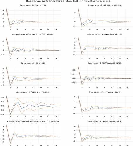
We also show the impulse responses of own country shocks in Figure 1.¹² Let us look at the results in Figure 1 to explain the results of own country shocks. For example, USA’s own country shocks take about 6 months to fully absorb in its forecast revision. On the other hand, it takes a longer time to incorporate the shock completely into China’s revision. We see similar results in other countries as well. These are clear indications of rigidity in forecast revisions although the time to absorb information varies from one country to another.

Figure 1. Generalized impulse responses of forecast revisions: own-country responses. (In percentage points, with two standard deviation confidence bands.).

5. Conclusions

In this study, we explored information rigidity in inflation forecasts utilizing a survey data set previously unexploited by researchers. Our main findings are as follows:

1. In general, we found weak evidence of information rigidity in the data set. We also found evidence of overreaction to new information signified by statistically significant negative coefficient values (Table 3, Table 4 and Table 5). We did not find significant differences in rigidity between the Developed and the Developing countries as evidenced by both forecast error and forecast revision-based tests.

2. In order to understand information rigidity during the financial crisis period of 2007, we ran two regressions. First, we ran the regression of the recession period (January 2007 – December 2012) only (Table 6). We found evidence of information rigidity at the 6M horizon, but not at the 3M horizon. Second, we ran the regression of the whole period using recession period as a dummy variable (Table 7). The dummy for the recession is positive and significant in all the groups signifying the presence of rigidity. We did not find statistically significant evidence of information acquisition speeding up during the recession period. We also perform Wald test to understand if the revisions during the recession period are different from the non-recession period. The results are mixed. We reject the null of no difference at the 3M, but could not reject the null at the 6M revisions.

3. We found evidence of cross-country correlation in forecast revisions (Table 8 and Table 9). Forecast revisions depend on both own country and cross-country lagged revisions. In general, we found that inflation revisions in any country prompt revisions in other countries both developed and developing, although with varying magnitudes. Therefore, one source of rigidity is not to incorporate overseas events in forecast revisions quickly and completely.

Disclosure statement

All authors certify that they have no affiliations with or involvement in any organization or entity with any financial interest or non-financial interest in the subject matter or materials discussed in this manuscript.

Additional information

Funding

The work was supported by the King Fahd University of Petroleum and Minerals [IN171019]

Notes

1. Angeletos et al. (2021) show that forecasters tend to underreact for the first few quarters following a shock but over-shoot later on, which they called delayed overreaction. Their investigation supports the combination of dispersed, noisy information and over-extrapolation type models while discounts the other theories. Kohlhas and Walther (2018) also propose a framework to reconcile the contradiction of underreaction and overreaction in survey data. Baker et al. (2020) shows that degree of information rigidity becomes smaller after a natural disaster shock supporting two-agent type model of information updating. Tsiaplias (2020) also shows that information rigidity depends on type of agents, one who updates regularly, and one who does not update except after large shocks. Other explanations are also proposed in the literature.

2. We follow IMF country classification in general. Czech Republic has been classified as developed by World Bank since 2006. Four Asian tigers have been classified as developed since 1997 by IMF.

3. The 25 developed countries are Australia, Austria, Belgium, Canada, Czech Republic, Denmark, Euro Area, Finland, France, Germany, Greece, Hungary, Ireland, Italy, Japan, Netherlands, New Zealand, Norway, Poland, Portugal, Spain, Sweden, Switzerland, United Kingdom, United States. The 18 developing countries are Argentina, Brazil, Chile, China, Colombia, Hong Kong, India, Indonesia, Mexico, Philippines, Russia, Singapore, South Africa, South Korea, Taiwan, Thailand, Turkey, Venezuela.

4. Consensus survey data carry unique information, as these are the opinions of experts, and not the public in general. Survey data are used as a proxy to unobservable expectations in economic models. Many central banks, businesses and academic institutions conduct regular surveys of experts to collect information on different variables, like interest rates, exchange rates, GDP growth rates, inflation rates, current accounts, unemployment rates, industrial production, etc.

5. Forecasts for GDP, CPI and current account are based on samples which typically range between 15–20 in this dataset. Unlike Consensus Forecasts, the journal does not publish individual forecasts. It only publishes the consensus forecasts.

6. This section is adopted from Loungani et al. (2013).

7. M is used as a shorthand notation for month.

8. We use 10 countries for the variance decomposition exercise mainly to conform with earlier studies so we can compare the results. We add 3 new countries to check for new results on the cross country forecast dependence.

9. Calculation: Sticky information model: Coefficient: a₁ = 0.37. Information rigidity: λ= a₁/(1+a₁) = 0.036. Duration of update: 1/(1-λ) = 1.04 quarters. Other numbers are calculated the same way.

Noisy information model: G = 1/(1+a₁) = 0.73. Other numbers are calculated the same way.

10. We do not have data at the individual country level to identify the recession period for each country separately.

11. The list of countries here are a mixture of the major developed (USA, Japan, Germany, UK, France and S. Korea) and the major developing economies (China, India, Russia and Brazil). These countries have bigger external sectors (export and import) as well. The purpose of this exercise is to show how information shocks, both domestic and foreign, affect forecast revision. One can expand the list of countries or choose other countries based on the interest.

12. Results of the cross-country impulse responses are available upon request.

References

- Abarbanell, J. S., & Bernard, V. L. (1992). Tests of analysts’ overreaction/under reaction to earnings information as an explanation for anomalous stock price behavior. Journal of Finance, 47(3), 1181–22. https://doi.org/10.1111/j.1540-6261.1992.tb04010.x
- Amir, E., & Ganzach, Y. (1998). Overreaction and under reaction in analysts’ forecasts. Journal of Economic Behavior and Organization, 37(3), 333–347. https://doi.org/10.1016/S0167-2681(98)00092-4
- Angeletos, G. M., Huo, Z., & Sastry, K. A. (2021). Imperfect macroeconomic expectations: Evidence and theory. NBER Macroeconomics Annual, 35(1), 1–86. https://doi.org/10.1086/712313
- Ashiya, M. (2002). Accuracy and rationality of Japanese institutional forecasters. Japan and the World Economy, 14(2), 203–213. https://doi.org/10.1016/S0922-14250200004-X
- Ashiya, M. (2003). Testing the rationality of Japanese GDP forecasts: The sign of forecast revision matters. Journal of Economic Behavior and Organization, 50(2), 263–269. https://doi.org/10.1016/S0167-26810200051-3
- Ashiya, M. (2006). Testing the rationality of forecast revisions made by the IMF and the OECD. Journal of Forecasting, 25, 25–36. https://doi.org/10.1002/for.979
- Baker, S. R., McElroy, T. S., & Sheng, X. S. (2020). Expectation formation following large unexpected shocks. Review of Economics and Statistics, 102(2), 287–303. https://doi.org/10.1162/rest_a_00826
- Beck, N., & Katz, J. N. (1996). Nuisance vs. substance: Specifying and estimating time-series–cross-section models. Political Analysis: An Annual Publication of the Methodology Section of the American Political Science Association, 6, 1–36. https://doi.org/10.1093/pan/6.1.1
- Bordalo, P., Gennaioli, N., Ma, Y., & Shleifer, A. (2020). Overreaction in macroeconomic expectations. American Economic Review, 110(9), 2748–2782. https://doi.org/10.1257/aer.20181219
- Clements, M. P. (1995). Rationality and the role of judgment in macroeconomic forecasting. The Economic Journal, 105(429), 410–420. https://doi.org/10.2307/2235500
- Clements, M. P. (1997). Evaluating the rationality of ?xed-event forecasts. Journal of Forecasting, 16(4), 225–239. https://doi.org/10.1002/SICI1099-131X19970716:4<225:AID-FOR656>3.0.CO;2-L
- Coibion, O., & Gorodnichenko, Y. (2012). What can survey forecasts tell us about information rigidities? Journal of Political Economy, 120(1), 116–159. https://doi.org/10.1086/665662
- Coibion, O., & Gorodnichenko, Y. (2015). Information rigidity and the expectations formation process: A simple framework and new facts. American Economic Review, 105(8), 2644–2678. https://doi.org/10.1257/aer.20110306
- Dovern, J. U., Fritsche, P., Loungani, N., Tamirisa, & Tamirisa, N. (2015). Information rigidities: Comparing average and individual forecasts for a large international panel. International Journal of Forecasting, 31(1), 144–154. https://doi.org/10.1016/j.ijforecast.2014.06.002
- Driscoll, J., & Kraay, A. C. (1998). Consistent covariance matrix estimation with spatially dependent panel data. Review of Economics and Statistics, 80(4), 549–560. https://doi.org/10.1162/003465398557825
- Ehrbeck, T., & Waldmann, R. (1996). Why are professional forecasters biased? Agency versus behavioral explanations. The Quarterly Journal of Economics, 111(1), 21–40. https://doi.org/10.2307/2946656
- Harvey, D. I., Leybourne, S. J., & Newbold, P. (2001). Analysis of a panel of UK macroeconomic forecasts. The Econometrics Journal, 4(1), S37–S55. https://doi.org/10.1111/1368-423X.00052
- Isiklar, G., Lahiri, K., & Loungani, P. (2006). How quickly do forecasters incorporate news? Evidence from cross-country surveys. Journal of Applied Econometrics, 21(6), 703–725. https://doi.org/10.1002/jae.886
- Jongen, R., Verschoor, W. F. C., & Wolff, C. C. P. (2008). Foreign exchange rate expectations: Survey and synthesis. Journal of Economic Surveys, 22(1), 140–165. https://doi.org/10.1111/j.1467-6419.2007.00523.x
- Kohlhas, A., & Broer, T. (2019). Forecaster (Mis-)Behavior. IIES miméo.
- Kohlhas, A., & Walther, A. (2018). Asymmetric attention. IIES miméo.
- Loungani, P. (2001). How accurate are private sector forecasts? Cross-country evidence from consensus forecasts of output growth. International Journal of Forecasting, 17(3), 419–432. https://doi.org/10.1016/S0169-20700100098-X
- Loungani, P., Stekler, H., & Tamirisa, N. (2013). Information rigidity in growth forecasts: Some cross-country evidence. International Journal of Forecasting, 29(4), 605–621. https://doi.org/10.1016/j.ijforecast.2013.02.006
- Mackowiak, B., & Wiederholt, M. (2009, June). Optimal sticky prices under rational inattention. American Economic Review, 99(3), 769–803. https://doi.org/10.1257/aer.99.3.769
- Mankiw, N. G., & Reis, R. (2002, November). Sticky information versus sticky prices: A proposal to replace the new keynesian phillips curve. The Quarterly Journal of Economics, 117(4), 1295–1328. https://doi.org/10.1162/003355302320935034
- Miah, F., Ali Khalifa, A., & Hammoudeh, S. (2016). Further evidence of rationality of interest forecast. Economic Modelling, 54(April 2016), 574–590. https://doi.org/10.1016/j.econmod.2015.12.036
- Nordhaus, W. D. (1987). Forecasting ef?ciency: Concepts and applications. The Review of Economics and Statistics, 69(4), 667–674. https://doi.org/10.2307/1935962
- Scotese, C. A. (1994). Forecast smoothing and the optimal under-utilization of information at the federal reserve. Journal of Macroeconomics, 16(4), 653–670. https://doi.org/10.1016/0164-07049490005-1
- Sims, C. A. (2003). Implications of rational inattention. Journal of Monetary Economics, 50(3), 665–690. https://doi.org/10.1016/S0304-39320300029-1
- Stekler, H. O., & Talwar, R. M. (2013). Forecasting the downturn of the great recession. Business Economics, 48(2), 113–120. https://doi.org/10.1057/be.2013.4
- Tsiaplias, S. (2020). Time-Varying consumer disagreement and future inflation. Journal of Economics Dynamics & Control, 116(C), 103903. https://doi.org/10.1016/j.jedc.2020.103903
- Woodford, M. (2001). Imperfect common knowledge and the effects of monetary policy,” phelps, princeton university press, 2002: In Honor of Edmund S. In P. Aghion, R. Frydman, J. Stiglitz, & M. Woodford. (Eds.), Knowledge, information, and expectations in modern macroeconomics (pp. 23–58). https://doi.org/10.1515/9780691223933-004