Manufacturing sector’s growth in Tanzania: Empirical lessons from macroeconomic factors, 1970–2021

Abstract

The study investigates the Tanzania manufacturing sector’s growth with a view to provide empirical lessons from macroeconomic factors with limited political regimes reflections. A vector error collection model was used to assess the influence of foreign direct investments (FDI), inflation (INF), export of product (EXP), power supply (PS), government expenditure (GoE), nominal lending interest rate (IRL), population growth rate (PGR) and exchange rate (EXR). The estimated value of the coefficient measuring the speed of adjustment toward long-run equilibrium is statistically significant and negative, implying that 41.6% of the short-run shocks can be corrected back to the long-run equilibrium immediately in the following year so has to prevent the model from explosion. Signs of INF, PS and IRL in the model estimation conform to expectations. Moreover, reducing production costs, increasing the trade openness, attracting FDI, offering appropriate government incentives and management of the foreign exchange rate have potentials of boosting the Tanzania’s economic growth. Thus, the government in collaboration with other stakeholders should work toward making the Tanzania manufacturing sector’s growth more competitive by creating conducive business environment that will lead to multiplier effects.

Keywords:

• macroeconomic variables
• political settlement
• conducive business environment
• competitiveness

PUBLIC INTEREST STATEMENT

Tanzania has potentials of reinforcing its economic structure and improve performance of the main sectors, manufacturing being one of it. The performance of Tanzania’s manufacturing sector has remained stagnant compared to other sectors of the economy, such as service and tourism. Based on Five-Years Development Plan 2020/21–2025/26 (FYDP III) and priorities of fifth and sixth political regimes, industrialization and investment remained hot development agenda. This study attempts to offer empirical lessons and slightly reflect on political regimes performance with regard to the influence of FDI, INF, EXP, PS, GoE, IRL, PGR and EXR on the manufacturing sector’s growth in Tanzania between 1970 and 2021. Enhanced implementation of Sustainable Industrial Development Policy (SIDP) is vital while effective participation of the private sector is needed to support state efforts. Industrial sector focusing on the growth potentials and competitiveness is needed linking pertinent economic activities that are pro-poor such as agriculture.

1. Introduction

Industrialization is a result of the technological change interaction, specialization and trade (Lugina et al., 2022). Good infrastructure, efficient communication, and educated labour force facilitate the promotion of rapid industrial development (Ibrahim et al., 2022). The industrial revolution transformed agriculture and handcrafts economies into mechanized manufacturing and large-scale industries (Gui Diby & Renard, 2015). This transformation led to the creation of new machines, advanced power sources and improved ways of organizing work, hence higher productivity which led to the rise of world economy structure (Gray, 2013; J. Rweyemamu, 1973).

According to the United Nations (2008), the manufacturing sector comprises of establishments that engaged in the physical or chemical transformation of materials, substances, or components into new products. The global manufacturing over the last two decades has been manifested by notable higher growth in the developing countries compared to the developed or industrialized countries. Contrary to developing nations, most of the developed economies prioritized the industrial development strategy aiming at stimulating their manufacturing sector (Sokunle et al., 2017). They primarily focused on modern manufacturing technologies (digitalized) and the application of information and communication technologies (ICTs). The trends of integrating ICTs in the manufacturing industry are viewed as the fourth industrial revolution, named as “Industry 4.0” (Zhang et al., 2014).

A notable success in the manufacturing output and stable economic growth was seen recently in most African countries while a decline and fluctuating trend were also noted in others. Moreover, the gross domestic product (GDP) share of manufacturing declined from 18% to 11% in 1975 and 2015 respectively, while the manufacturing production has almost doubled since 2000, from 85 USD billion in 2000 to 160 USD billion in 2015. African manufacturing growth rate was 3.5% in real terms over the past decade, more than developed countries (ATF, 2018). Back then, Lipumba and Kasekende (1991) reported that the key driver behind the “African growth miracle” is the substantial expansion of the service sector. Essentially, the post 2000 period of growth in Africa observed the declining importance of agriculture and manufacturing and a notable increase in the importance of services.

The Tanzania economy is diversified with a high prospective growth, though there are opportunities which remain unexploited (URT, 2019). The performance of Tanzania’s manufacturing sector has remained stagnant compared to other sectors of the economy despite the fact that various efforts and strategies were suggested such as the adoption of Development Vision 2025 in 1999, introduction of the Integrated Industrial Development Strategy (IIDS) in 2011, Blueprint 2018 with a view to create conducive environment for investments and business, promoting investment and trade for Special Economic Zones (SEZs) and Export Processing Zones (EPZs), Strengthening Research and Development (R&D) and promoting Micro, Small and Medium Entrepreneurs (MSMEs). Recent trends revealed the relatively low manufacturing sector’s contribution to the GDP (Mwang’onda et al., 2018).

Tanzania has put in place a medium-term framework with a Five-Years Development Plan 2020/21–2025/26 (FYDP III) being the third and the last plan toward the Development Vision 2025. The FYDP III aims at strengthening industrialization as a basis for the export-oriented growth, as well as focusing on producing new products and market; also transforming the country into a manufacturing hub of East, Southern and Central Africa, as well as significantly increase Tanzania’s share of the international trade. For the manufacturing sector, the FYDP III aims at accelerating the real growth rate from 5.6% 2020/21 to 7.0% by 2025/26 and increase share of the GDP (at current price) from 8.2% to 8.5%, share of total employment 6.8% to 12.8% and share of export earnings from 17.1% to 19.0%, respectively (URT, 2021). In this regard, emphasis on industrialization and investment was noted to be the hot development agenda particularly during the fifth and sixth political regimes, respectively. However, the Tanzania manufacturing sector’s development can be viewed and learnt from the 1960s after independence.

Then, it is worth noting that the manufacturing sector plays an important role for economic growth and sustainable development (Sokunle et al., 2017). There are numerous studies on factors affecting the manufacturing sector’s growth in both developed and developing economies (Azolibe, 2020; Chaudhry et al., 2013; Goedhuys & Sleuwaegen, 2010; Loto, 2012; Omotor, 2008; Oyati, 2010; Rana & Dowling, 1988; Sokunle et al., 2017). However, it was not clearly stipulated how the manufacturing sector’s growth relates to the pertinent macroeconomic variables while mixed evidences associated with the behavior of variables in different countries including Tanzania were revealed. Moreover, concrete evidences that attempt to compare a wider range of key variables and time period in terms of years in relation to magnitude of the manufacturing sector growth determinants are scant (Lugina et al., 2022).

There are limited studies that covered the post 1994 period in Tanzania specifically on the manufacturing sector’s growth. For instance, some useful studies were conducted by the World Bank (1991), URT (1965) and, Skarstein and Wangwe (1986) although, they were undertaken when the economy was still largely dominated by the state control. It is also worth mentioning that political settlement approach can widely be applied (Khan, 2018) and implications on industrial policy can also be drawn (Whitfield et al., 2015). Thus, with marginal political regimes echoes, this study attempts to shed more light on empirical lessons with regard to the influence of foreign direct investments, inflation, export of products, power supply, government expenditure, interest rate, population growth rate and exchange rate on the manufacturing sector’s growth in Tanzania between 1970 and 2021.

2. Theoretical and conceptual standpoint

The study was guided by two theories which were accelerator and neoclassical theory of investment and growth. The theoretical framework was adapted from Sokunle et al. (2017). The earlier theory is centered on a linkage between capital stock and the level of output of the firm while the later provides a new insight on the causes of variations in investment. Based on the theories factors such as, interest rates, investments, and variations in the private sector had a profound effect on manufacturing sector growth (Rana & Dowling, 1988).

In this regard, the concept and theories of the investment and growth were found to be relevant to support the theoretical foundation of the study. In other words, the paper takes them as a guide, without completely ignoring external factors, from which important points have been noted in the study approach and reflected in the findings. The manufacturing growth model, for instance, was reported to use factors such as FDI inflows, interest rates, inflation and government incentives (Arthur & Addai, 2022; Chaudhry et al., 2013; Moussa et al., 2019; Sokunle et al., 2017). While some other specific macroeconomic variables were left behind, such as unemployment rate (Onakoya, 2018); however, proxy were considered, such as population growth rate.

Based on the reviewed studies, we adapted the model of manufacturing sector growth which is having a total of eight independent variables namely FDIs, inflation, exports of product, power supply, government expenditure, interest rate, population growth rate and exchange rate which are influencing manufacturing sector. The selection of the model was based on the fact that for a country to experience high growth in manufacturing sector, it should put more efforts in investments on infrastructure (power supply), encourage foreign investments and monitor price fluctuation (inflation) and promote export of products. In the same vein, government incentive, interest rate, population growth rate and exchange rate were also vital.

According to the scope of other cited studies on the determinants of manufacturing sector growth, some revealed that variables were not satisfactory (not statistically significant) in explaining manufacturing sector in their respective countries. Log-linear regression model can reduce heteroscedasticity (Gujarati, 2004) hence was used as demonstrated by different scholars including but not limited to Singh and Kumar (2022) and Bekele and Haile (2020). However, the combination of linear, log-linear and non-linear regression models is possible given the nature of variables and timeframe given respective study objective (Singh & Kumar, 2021). The coverage and scope of the current study ranged from 1970 to 2021. This range of years seemed reasonable and statistically sound.

3. Methodology

3.1. Design and data sources

Quantitative research design was used to analyze the Tanzania manufacturing sector’s growth dynamics in relation to the selected macroeconomic variables using time series data. Time series analysis was appropriate in observing the trends during different regimes and relationship of these variables over time between 1970 and 2021. Secondary data was the main source gathered from the National Bureau of Statistics (NBS), Bank of Tanzania (BOT), Economic Surveys and World Development Indicators (WDI).

3.2. Model and variables

The manufacturing sector’s growth in terms of manufacturing value added (MVA) was used as a dependent variable while foreign direct investments (FDI), inflation (INF), export of product (EXP), power supply (PS), government expenditure (GoE), nominal lending interest rate (IRL), population growth rate (PGR) and exchange rate (EXR) as the independent variables.

The general function model for this study is given by;

MVA = f(FDI, INF, EXP, PS, GoE, IRL, PGR, EXR)

For the purpose of estimation, the modified regression equation is presented as follows;

(1) $\mathrm{M}\mathrm{V}{\mathrm{A}}_{\mathrm{t}}={\beta }_0+{\beta }_1{\left(\mathrm{F}\mathrm{D}\mathrm{I}\right)}_{\mathrm{t}}+{\beta }_2{\left(\mathrm{I}\mathrm{N}\mathrm{F}\right)}_{\mathrm{t}}+{\beta }_3{\left(\mathrm{E}\mathrm{X}\mathrm{P}\right)}_{\mathrm{t}}+{\beta }_4{\left(\mathrm{P}\mathrm{S}\right)}_{\mathrm{t}}+{\beta }_5{\left(\mathrm{G}\mathrm{o}\mathrm{E}\right)}_{\mathrm{t}}+{\beta }_6{\left(\mathrm{I}\mathrm{R}\mathrm{L}\right)}_{\mathrm{t}}+{\beta }_7{\left(\mathrm{P}\mathrm{G}\mathrm{R}\right)}_{\mathrm{t}}+{\beta }_8{\left(\mathrm{E}\mathrm{X}\mathrm{R}\right)}_{\mathrm{t}}+{\epsilon }_{\mathrm{t}}$(1)

Equation (1)(1) $\mathrm{M}\mathrm{V}{\mathrm{A}}_{\mathrm{t}}={\beta }_0+{\beta }_1{\left(\mathrm{F}\mathrm{D}\mathrm{I}\right)}_{\mathrm{t}}+{\beta }_2{\left(\mathrm{I}\mathrm{N}\mathrm{F}\right)}_{\mathrm{t}}+{\beta }_3{\left(\mathrm{E}\mathrm{X}\mathrm{P}\right)}_{\mathrm{t}}+{\beta }_4{\left(\mathrm{P}\mathrm{S}\right)}_{\mathrm{t}}+{\beta }_5{\left(\mathrm{G}\mathrm{o}\mathrm{E}\right)}_{\mathrm{t}}+{\beta }_6{\left(\mathrm{I}\mathrm{R}\mathrm{L}\right)}_{\mathrm{t}}+{\beta }_7{\left(\mathrm{P}\mathrm{G}\mathrm{R}\right)}_{\mathrm{t}}+{\beta }_8{\left(\mathrm{E}\mathrm{X}\mathrm{R}\right)}_{\mathrm{t}}+{\epsilon }_{\mathrm{t}}$(1) was transformed through natural logarithm as shown in equation 2(2) $\mathrm{l}\mathrm{n}\mathrm{\_}\mathrm{M}\mathrm{V}\mathrm{A}={\beta }_0+{\beta }_1\mathrm{l}\mathrm{n}\mathrm{\_}(\mathrm{F}\mathrm{D}\mathrm{I}{)}_{\mathrm{t}}+{\beta }_2(\mathrm{I}\mathrm{N}\mathrm{F}{)}_{\mathrm{t}}+{\beta }_3\mathrm{l}\mathrm{n}\mathrm{\_}(\mathrm{E}\mathrm{X}\mathrm{P}{)}_{\mathrm{t}}+{\beta }_4\mathrm{l}\mathrm{n}\mathrm{\_}(\mathrm{P}\mathrm{S}{)}_{\mathrm{t}}+{\beta }_5\mathrm{l}\mathrm{n}\mathrm{\_}(\mathrm{G}\mathrm{o}\mathrm{E}{)}_{\mathrm{t}}+{\beta }_6(\mathrm{I}\mathrm{R}\mathrm{L}{)}_{\mathrm{t}}+{\beta }_7\mathrm{l}\mathrm{n}\mathrm{\_}(\mathrm{P}\mathrm{G}\mathrm{R}{)}_{\mathrm{t}}+{\beta }_8\mathrm{l}\mathrm{n}\mathrm{\_}(\mathrm{E}\mathrm{X}\mathrm{R}{)}_{\mathrm{t}}+{\epsilon }_{\mathrm{t}}$(2) . Log transformation very often reduces heteroscedasticity when compared to usual regression this is due to the fact that it compresses the scales in which the variables are measured (Gujarati, 2004). The coefficients of log transformed model provide elasticity of the manufacturing sector’s growth against macroeconomic variables under examination. For the case of skewed data, log transformation tends to convert skewed data to almost conform to normality (Feng et al., 2014) hence adapted by the study.

(2) $\mathrm{l}\mathrm{n}\mathrm{\_}\mathrm{M}\mathrm{V}\mathrm{A}={\beta }_0+{\beta }_1\mathrm{l}\mathrm{n}\mathrm{\_}(\mathrm{F}\mathrm{D}\mathrm{I}{)}_{\mathrm{t}}+{\beta }_2(\mathrm{I}\mathrm{N}\mathrm{F}{)}_{\mathrm{t}}+{\beta }_3\mathrm{l}\mathrm{n}\mathrm{\_}(\mathrm{E}\mathrm{X}\mathrm{P}{)}_{\mathrm{t}}+{\beta }_4\mathrm{l}\mathrm{n}\mathrm{\_}(\mathrm{P}\mathrm{S}{)}_{\mathrm{t}}+{\beta }_5\mathrm{l}\mathrm{n}\mathrm{\_}(\mathrm{G}\mathrm{o}\mathrm{E}{)}_{\mathrm{t}}+{\beta }_6(\mathrm{I}\mathrm{R}\mathrm{L}{)}_{\mathrm{t}}+{\beta }_7\mathrm{l}\mathrm{n}\mathrm{\_}(\mathrm{P}\mathrm{G}\mathrm{R}{)}_{\mathrm{t}}+{\beta }_8\mathrm{l}\mathrm{n}\mathrm{\_}(\mathrm{E}\mathrm{X}\mathrm{R}{)}_{\mathrm{t}}+{\epsilon }_{\mathrm{t}}$(2)

where β₀ represents constant, β_1, β_2, β_3, β_4, β_5, β_6, β₇ and β₈ represent estimated coefficients at time t and ε_t represents error term. Moreover, ln_MVA is logarithm of manufacturing sector growth; ln_FDI is logarithm of foreign direct investments; INF is the inflation rate; ln_EXP is logarithm of export of products (manufactured products), ln_PS is the logarithm of power supply, ln_GoE is logarithm of government expenditure, IRL is the nominal lending interest rate, ln_PGR is logarithm of population growth rate and ln_EXR is logarithm of exchange rate. Table 1 presents the studied variables and the expected sign basing on the theory.

Table 1. Variable, unit of measurement and expected signs

Variable	Unit of Measurement	Expected Sign
Manufacturing Sector’s Growth	MVA (USD Million)	Dependent variable
Foreign Direct Investments	Inflows (USD Million)	Positive
Inflation Rate	Rise in the price level (Percent)	Negative
Export of Product	Manufactured products (USD Million)	Positive
Power Supply	Electricity generated (KWH Million)	Positive
Government Expenditure	Spending (USD Million)	Positive
Nominal Lending Interest Rate	Money rate (Percent)	Negative
Population Growth Rate	Rise in the population (Percent)	Positive
Exchange Rate	Real effective exchange rate (Percent)	Negative

3.3. Data analysis

Basing on the types of data, descriptive and trend analysis were done for growth rates computations and by using pictorial presentation, respectively. The study utilized various tests such as; normality tests, unit root test for stationarity. Then, co-integration tests were performed as well as granger causality test.

Normality properties (i.e., efficient of mean, variance, standard deviation, skewness and kurtosis) were established. Moreover, unit root test was used to examine the stationarity of the variables under the study. A time series data is said to be stationary if its value tends to return to its long-run average value and properties of data series such as mean, variance and covariance are not affected by the change in time only (Shrestha & Bhatta, 2018). This was done by using the Augmented Dickey–Fuller (ADF) test which adds the largest values of the variable.

Co-integration refers to a long-run relationship of variables linked to form an equilibrium relationship when the individual series are inherently non-stationary in their levels but became stationary after being differentiated. In the course of managing regression analysis, a test for co-integration is applied to avoid spurious regression results. The method for testing the existence of long-run relationship between variables in the model for this study is Johansen co-integration test which also gives the maximum rank of co-integration.

The co-integration term is specifically termed as error correction term because any deviation from long-run equilibrium is corrected through a series of partial short-run adjustments. The error correction term represents the long-run relationship. A negative and significant coefficient of the error correction term indicates the presence of long-run causal relationship. The size of the error correction term indicates the speed of adjustment of any disequilibrium toward a long-run equilibrium.

The determinants of co-integration relationship were determined, the next step was to estimate the level of the manufacturing sector’s growth by using Error Correction Model (ECM). The ECM for estimation reads as follows; in estimating an ECM, the residual from the estimation of equation should be subjected to standard ADF unit root test. Akaike Information Criteria (AIC) was used as a guide to reduce the model by eliminating highly insignificant lags and variables in each turn of the repeated OLS estimation process while maintaining the model that will best fit the data.

The granger causality test was performed for the model in order to examine the granger causal relationship between the variables under examination. F-statistic was used as a testing criterion where by the hypothesis of the statistical significance of each explanatory variable was tested.

A common diagnostic test was used before applying the model to test the significance of the slopes and analyzing the regressed result of the model equation; testing the presence of heteroscedasticity, Variance Inflation Factor (VIF) test was conducted to test the multicollinearity. Also, Ramsey RESERT was applied to assess whether the model is improperly specified or not. Furthermore, diagnostic checks or post estimation involves testing the autocorrelation by using Lagrange multiplier test and Jarque-Bera test were applied for normality test.

4. Results and discussion

4.1. Descriptive statistics and trend

Descriptive statistics of the MVA, FDI, INF, EXP, PS, GoE, IRL, PGR and EXR are presented in Table 2. Basing on the measure of symmetry results, values are positively skewed implying that the data are normally distributed.

Table 2. Descriptive statistics results

Variable	Mean	Maximum	Minimum	SD	Kurtosis	Skewness
MVA	2,577.44	5,627.86	721.46	1,411.45	1.92	0.37
FDI	514.78	2,087.26	1.52	594.86	2.92	1.00
INF	15.22	36.32	3.29	11.13	1.77	0.60
EXP	909.10	7,798.00	30.10	1,450.76	12.98	3.07
PS	2,873.79	8,580.80	395.00	2,399.76	2.56	0.92
GoE	1,033.34	5,074.15	9.78	1,206.09	4.60	1.53
IRL	16.66	35.95	7.50	7.52	3.15	0.84
PGR	3.03	3.89	1.88	0.41	3.11	(0.38)
EXR	771.32	2,298.20	6.90	792.31	2.15	0.67

MVA = Manufacturing Sector’s growth, FDI = Foreign Direct Investments, INF = Inflation Rate, EXP = Export of Products (manufactured products), PS = Power Supply, GoE = Government Expenditure, IRL = Nominal Lending Interest Rate, PGR = Population Growth Rate and EXR = Exchange Rate and SD = Standard Deviation.

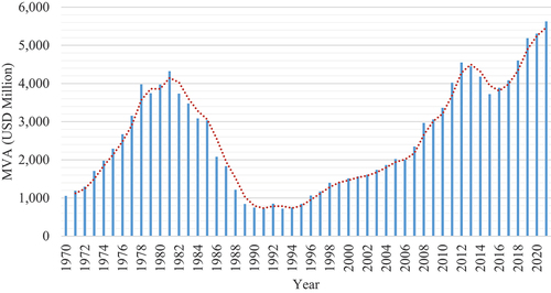
There has been ups and downs trend in the MVA expressed as proxy indicator of the manufacturing sector’s growth (MG) in Tanzania (Figure 1). The significant growth of the sector in terms of gross output was realized in 1970s, the peak was observed in 1981, and then dropped over the period from 1982 to 1991. This is in line with what was reported by Mnenwa and Maliti (2009). Moreover, the increasing trend can also be noted from 1995 to 2012 and from 2017 during the fifth political regime (Figure 1).

Figure 1. Trend of manufacturing value added in Tanzania.

The manufacturing sector contribution to the overall GDP of the country has averaged 8% over the last decade; however, activities within the sector have been registered an annual growth rate of over 4% and the sector is nowadays the third most important to the economy behind agriculture and tourism. The manufacturing sector generated USD 4.1 billion (8% of the GDP) in 2018 compared to USD 3 billion in 2014, representing an increase of 39%. Tanzania’s economy depends much on agriculture as agriculture accounted for 30.1% of the GDP in 2018, the manufacturing industrial activity focuses mainly on the processing of locally produced agricultural products (URT, 2019). Basing on the World Economic Forum, the statistics indicates that the leading industrial activity is food processing, followed by textiles and clothing, chemicals and others including; beverages, leather and leather products, paper and paper products, publishing and printing as well as plastics.

The development of manufacturing can be traced back to the 1960s especially after the Arusha declaration in 1967. The main agenda of the Arusha declaration was socialism and self-reliance. Major means of production came under state control after the introduction of state led import substitution and state led expansion of manufacturing. In 1971, price control came into application in order to fix and oversee prices of limited number of manufactured goods (Mongi, 1980). Industrial production was basically meant to meet the basic necessities of residents, intermediate and capital goods for the economy. Between 1973 and 1974, there was a shortage of foreign exchange, as a result, Tanzania experienced a shortage of balance of payment which subsequently affected the industrial production. In the late 1978, we observed a downward trend which may be attributed to the Tanzania and Uganda war as well as the breakup of the East African Community (EAC). Tanzania had to defend itself following the invasion of Iddi Amini. A war drained the Tanzania’s accumulated national resources that could have been dedicated for the national development including manufacturing sector. Amid the complexity of this crunch, the country experienced a drop-in real growth rate between 1981 and 1983 which necessitated the need for recovery programs (Msami & Wangwe, 2016). One of the initiated recovery programs is the National Survival Program (NSP) in 1981–1982 aimed at overcoming the economic crisis by using national resources (Muganda, 2004).

In 1986, the Tanzania government adopted the policy of Structural Adjustments Programs (SAPs) devised by the International Financial Institutions (IFI) for industrial development. Also, the Government adopted the Economic Recovery Programs (ERP) aimed at bringing economic stability and fasten the structural reforms so as to attain sustainable balance of payment, reduce inflation, correct budget deficits, improve the microeconomic policy framework and raise incentives for the agricultural producers (Wangwe et al., 2014). The programs conveyed the role of the market in an economy by putting empasis on removinggovernment contol and involvementin trading and investment, and by that time the private sectors were allowed to involve themselves in the manufacturing sector activities (Mussa, 2014). The outcome of this programs was observed between 1987 and 1989 with a decline in 1990 followed by the increase in 1990. However, during that time, trade liberalization came into action which hindered most developing countries including Tanzania due low their competitiveness of the local industries leading to significant loss of local industries against the low cost imports (Msami & Wangwe, 2016; Mussa, 2014).

The decline of manufacturing sector’s growth could be tracked between 1992 and 1995, followed by recovery after 1995 (URT, 2020). In this regard, the breakdown of the manufacturing production intensified during the economic crisis period. Following major economic reforms adopted in 1986, the sector has been subjected to substantial re-structuring aimed at increased growth capacity utilization and overall efficiency. The Tanzania economic liberalization through 1990s boosted the economy’s manufacturing sector. It will be recalled that after the introduction of import substitution and basic industrialization strategies; the Tanzanian manufacturing sector became a fast-growing sector (Kahyarara, 2013).

The Tanzania’s industrialization period in is noticeable after instituting and implementing the Sustainable Industrial Development Policy of 1996 (SIDP). The Government intended to have a sector geared toward human development, job creation, economic transformation for achieving sustainable economic growth and environmental sustainability (URT, 1996). The implementation of this policy was splitted in three phases; phase I (1996–2000) which accord on consolidating and rehabilitating the existing industries through capital, financing and management restructuring; phase II (2000–2010) aimed at establishing intermediate goods and light capital goods and machinery industries, promoting manufacturing exports and establishing technological innovation for natural resources exploitation; and phase III (2010–2020) which provides major investment in basic capital goods.

The Tanzania manufacturing sector’s growth, can also be summarized in five political regimes soon after independence with selected economic indicators (Table 3). The first political regime was mainly from 1964 to 1985, the economy (GDP growth rate) was growing at an average of 3% and the manufacturing growth rate with an average of 1.8%. During that period, FDI was not well emphasized as it accounted for an average of 5.7 USD and power supply on average was 677 KWH. In 1967, Tanzania introduced the Arusha declaration with the main agenda of socialism and self-reliance where by all major means of production were state controlled.

Table 3. Selected economic indicators during the five political regimes in Tanzania

Political Regime	GDP at C.P (TZS Mill.)	MVA (TZS Mill)	Growth Rate		FDI (USD Mill).	INF (%)	PS (KWH)
			MG (%)	GDP (%)
1964–1985	46,819	6,773	1.8	3.0	5.7	14.1	677
1985–1995	6,984,507	782,916	3.8	4.1	20.4	29.7	1,627
1995–2005	12,218,769	1,356,737	6.7	5.6	410.2	8.9	2,507
2005–2015	53,969,567	5,255,792	7.3	6.5	1,260.2	9.0	5,146
2015–2020	124,011,132	9,965,068	8.3	6.9	1,095.2	4.1	7,342

The second political regime was from 1985 to 1995, the GDP growth rate was on an average of 4.1% and the manufacturing growth rate was an average of 3.8% (Figure 2). The FDI on average were 20.4 USD and power supply on average accounted for 1,627 KWH. During this regime, most nationalized enterprises had suffered from the lack of foreign exchange for importation of necessary goods and competition from the world market. Hence, agenda of trade liberalization came into existence.

Figure 2. Manufacturing sector and GDP growth trend.

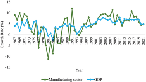
During the third political regime from 1995 to 2005, the GDP growth rate on average was 5.6% and the manufacturing sector’s growth rate of 6.7% on average. The foreign direct investments rose to an average of 410.2 USD and power supply on average accounted for 2,507 KWH. In 1995, Tanzania came up with national vision which is Development Vision of 2025 with a view to exploit national productive resources for national development. The vision foresees Tanzania to become a middle-income industrialized country with a high level of human development index combined by modernized and productive agro-industrial integrated to supportive industrial and service sectors. The main agenda of this regime was privatization.

The GDP growth rate on average during the fourth political regime (2005 to 2015) was 6.5% and the manufacturing growth rate was 7.3% on average. It’s during this fourth political regime where the foreign direct investments were much promoted with an average of 1,260.2 USD and power supply infrastructure was increased to an average of 2,507 KWH.

The fifth political regime took office from 2015 to 2020, the economy was growing at an average of 6.9% and the manufacturing growth rate was 8.3% on average. During this regime, foreign direct investments were also promoted with an average of USD 1,095.2 and power supply infrastructure was 7,342 KWH on average. The GDP growth led to a per-capita income of 1,063 USD; making Tanzania one of low-middle economies in Africa. The fifth regime put more emphasis on the industrialization gear as a hot development agenda.

In this regard, our reflections revealed that attractiveness of FDI observed can be attributed to the perceived democratic process which attracted more investors; both local and international. However, this should last longer even after the change of political regimes (Gray, 2013; R. Rweyemamu, 1979). Fluctuating trend of IFN was associated with different factors, such as political turmoil of 1982, the increase in money supply as a result of multiparty in 1992 and the uncertainty attributed to the Tanzania general elections. National level strategies have a role to play in encouraging domestic production and exports. Positive changes on EXP were attributed to the five-year development program which was addressed under the National Strategy for Growth and Reduction of Poverty (NSGRP) campaign, although did not last longer during the subsequent political regimes. Tanzania PS has a consistent rise as expected with its sharp increase from 2005 onward.

Thus, the trends in terms of the Tanzania manufacturing sector’s growth reflect the periods of industrial development in the post-independent Tanzania namely: a period of expansion, from 1974–1980; a period of collapse 1981–1990; a period of adjustment, privatization and re-structuring, 1991–1995 and industrialization era, 1996–2020. Regardless of the political regime, economic performance is highly influenced by public finance in different ways, such as funding policies, supporting the manufacturing industry and businesses both directly and indirectly, and lower production costs through infrastructure development and public services (Gray, 2015; Ibrahim et al., 2022).

4.2. Diagnostic test results

4.2.1. Unit root

For the macroeconomic data to have the feature of random walk, the presence of a unit root problem for each variable was checked to avoid the spurious results.

The ADF results revealed that all variables are non-stationary at all critical values (all levels) i.e., 1%, 5% and 10% and p-value are not significant at 5% level. In this case, further analyses were not possible to be performed (Table 4). Moreover, results in Table 5 show that after the first difference, all variables become stationary meaning that they have no unit root. Their t-statistics were significant in all levels. Basing on these, all variables were stationary and integrated in order one, that is, I (1) and are homogenous, hence the long-run relationship between variables using Johansen co-integration test were determined thereafter.

Table 4. Augmented Dickey–Fuller unit root test

Variable	Test Statistic	Critical Value			P-Value	Results
		1%	5%	10%
ln_MVA	−0.551	−3.579	−2.929	−2.6	0.8816	Non-Stationary
ln_FDI _ipo	−1.168	−3.579	−2.929	−2.6	0.6872	Non-Stationary
INF	−2.088	−3.579	−2.929	−2.6	0.2495	Non-Stationary
ln_EXP _ipo	−1.752	−3.579	−2.929	−2.6	0.4045	Non-Stationary
ln_PS	−0.921	−3.579	−2.929	−2.6	0.7809	Non-Stationary
ln_GoE	−1.109	−3.579	−2.929	−2.6	0.7116	Non-Stationary
IRL	−1.480	−3.579	−2.929	−2.6	0.5436	Non-Stationary
ln_PGR	−2.858	−3.579	−2.929	−2.6	0.0505	Non-Stationary

Table 5. Augmented Dickey–Fuller unit root test at first difference

Variable	Test Statistic	Critical Value			P-Value	Results
		1%	5%	10%
ln_MVA	−3.794	−3.579	−2.929	−2.6	0.003	Stationary
ln_FDI _ipo	−8.776	−3.579	−2.929	−2.6	0.000	Stationary
INF	−9.407	−3.579	−2.929	−2.6	0.000	Stationary
ln_EXP _ipo	−5.613	−3.579	−2.929	−2.6	0.000	Stationary
ln_PS	−5.662	−3.579	−2.929	−2.6	0.000	Stationary
ln_GoE	−6.269	−3.579	−2.929	−2.6	0.000	Stationary
IRL	−6.301	−3.579	−2.929	−2.6	0.000	Stationary
ln_PGR	−5.596	−3.579	−2.929	−2.6	0.000	Stationary

4.2.2. Heteroscedasticity

To detect the presence of heteroscedasticity, heteroscedasticity test was performed in this study. This test states that if the probability value of chi square is insignificant (greater than 0.05), then data has no heteroscedasticity problem. Basing on the probability of the chi-square which was greater than 0.05 (Table 6), there was a constant variance (no heteroscedasticity) in error terms. This was also in line with what was depicted by the graphs to mean that residuals were well distributed.

Table 6. Heteroscedasticity test results

Breusch–Pagan/Cook–Weisberg test for heteroskedasticity
Ho: Constant variance
Variables: fitted values of D1.ln_MVA
chi2(1) = 2.40
Prob > chi2 = 0.1212

4.2.3. Model misspecification and multicollinearity

Model specification test was also applied for the study to avoid biased coefficients and error terms. The powers of the fitted values of D.ln_MVA indicated that p-value of 0.2917 is not statistically significant different from zero. For this case, the model had no problem of misspecification nor omitted variables.

The VIF values from each of the explanatory variable are less than 5 (Table 7) implying the presence of moderate correlation between variables in the model hence no multicollinearity. Also, the correlation matrix helped to determine easily which variables might be correlated with each other by viewing the correlation coefficients between each variable in the model (Table 8).

Table 7. Variance inflation factor

Variable	VIF	1/VIF
D1.ln_GoE	1.78	0.561
D1.IRL	1.69	0.591
D1.ln_EXP_ipo	1.53	0.655
D1.ln_PS	1.30	0.771
D1.ln_PGR	1.26	0.796
D1.INF	1.11	0.902
D1.ln_FDI _ipo	1.10	0.905
Mean VIF	1.4

Table 8. Correlation matrix test

	D1.ln_MVA	D1.ln_FDI	D1.INF	D1.ln_EXP	D1.ln_PS	D1.ln_GoE	D1.IRL	D1.ln_PGR
D1.ln_MVA	1.000
D1.ln_FDI _ipo	0.148	1.000
D1.INF	−0.0405	−0478	1.000
D1.ln_EXP _ipo	−0.0391	−0.1874	−0.268	1.000
D1.ln_PS	−0.1098	0.070	−0.1289	’0.417	1.000
D1.ln_GoE	0.279	−0.081	−0.170	0.221	0.013	1.000
D1.IRL	−0.1884	0.005	0.089	’−0.0234	0.164	−0.584	1.000
D1.ln_PGR	−0.078	−0.0573	0.162	−0.331	−0.168	−0.235	−0.067	1.000

4.2.4. Determination of the number of lags

It was very important to select the proper lag length when performing regression by using restricted Vector Auto-Regression (VAR) which is Vector Error Correction Model (VECM). Thus, the selection order criteria such as sequential modified LR test statistic (LR), Final Prediction Error (FPE), Akaike Information Criterion (AIC), Hannan and Quinn Information Criterion (HQIC) as well as Schwarz’s Bayesian Criterion (SBIC) were used. Table 9 presents the selection order criteria results from 48 observations between 1976 and 2021.

Table 9. Selection-order criteria

Lag	LL	LR	df	p	FPE	AIC	HQIC	SBIC
0	−482.647				0.104421	20.4436	20.5615	20.7555
1	−104.677	755.94	64	0	0.000	7.36154	8.42224	10.1683*
2	’−22.9254	163.5	64	0	1.30E–07	6.62189	8.62543	11.9236
3	92.6565	231.16	64	0	3.00E–08	4.47265	7.41902	12.2693
4	218.505	251.7*	64	0	1.1e−08*	1.89561*	5.78482*	12.1872

Endogenous: ln_MVA, ln_FDI_ipo, INF, ln_EXP_ipo, ln_PS, ln_GoE, IRL and ln_PGR

Exogenous: _cons

Majority rule was used to select the parameter with optimal lag length. The number of lags in the model was determined according to LR, FPE, AIC and HQIC which suggested the optimal lag to be four (4), while Schwarz’s Bayesian Criterion (SBIC) suggest lag one (1). Basing on the majority rule, there are four (4) number of lags selected in this study.

4.3. Co-integration results

The Johansen co-integration test performed also involved both trace and maximum eigenvalue tests with the alternative hypothesis that: there is co-integration. But there is an exception for this test by differing the null hypothesis in the case of differing ranks. The main focus of the test results was on maximum rank, trace or maximum statistics and critical values (Table 10).

Table 10. Johansen tests for co-integration

Maximum Rank	Parms	LL	Eigen value	Trace Statistic	5% Critical Value
0	200	50.543879		335.9229	156.00
1	215	98.099511	0.86214	240.8116	124.24
2	228	135.84386	0.79251	165.3229	94.15
3	239	166.03293	0.71574	104.9448	68.52
4	248	186.64176	0.57629	63.7272	47.21
5	255	200.95116	0.44911	35.1083	29.68
6	260	211.70515	0.36115	13.6004*	15.41
7	263	217.49185	0.21425	2.027	3.76
8	264	218.50533	0.04135
0	200	50.543879		95.1113	51.42
1	215	98.099511	0.86214	75.4887	45.28
2	228	135.84386	0.79251	60.3781	39.37
3	239	166.03293	0.71574	41.2177	33.46
4	248	186.64176	0.57629	28.6188	27.07
5	255	200.95116	0.44911	21.508	20.97
6	260	211.70515	0.36115	11.5734	14.07
7	263	217.49185	0.21425	2.027	3.76
8	264	218.50533	0.04135

Sample: 1976–2021, Trend- Constant, Lags = 4 and Number of Observation = 48

At maximum rank zero, the trace statistics exceeds critical value. Likewise, maximum statistics exceeds critical value (Table 10). Thus, the null hypothesis was rejected under maximum rank zero, hence the study variables were co-integrated. After maximum rank zero, the other ranks state the null hypothesis that there is a co-integration of Equation (1(1) $\mathrm{M}\mathrm{V}{\mathrm{A}}_{\mathrm{t}}={\beta }_0+{\beta }_1{\left(\mathrm{F}\mathrm{D}\mathrm{I}\right)}_{\mathrm{t}}+{\beta }_2{\left(\mathrm{I}\mathrm{N}\mathrm{F}\right)}_{\mathrm{t}}+{\beta }_3{\left(\mathrm{E}\mathrm{X}\mathrm{P}\right)}_{\mathrm{t}}+{\beta }_4{\left(\mathrm{P}\mathrm{S}\right)}_{\mathrm{t}}+{\beta }_5{\left(\mathrm{G}\mathrm{o}\mathrm{E}\right)}_{\mathrm{t}}+{\beta }_6{\left(\mathrm{I}\mathrm{R}\mathrm{L}\right)}_{\mathrm{t}}+{\beta }_7{\left(\mathrm{P}\mathrm{G}\mathrm{R}\right)}_{\mathrm{t}}+{\beta }_8{\left(\mathrm{E}\mathrm{X}\mathrm{R}\right)}_{\mathrm{t}}+{\epsilon }_{\mathrm{t}}$(1) -2(2) $\mathrm{l}\mathrm{n}\mathrm{\_}\mathrm{M}\mathrm{V}\mathrm{A}={\beta }_0+{\beta }_1\mathrm{l}\mathrm{n}\mathrm{\_}(\mathrm{F}\mathrm{D}\mathrm{I}{)}_{\mathrm{t}}+{\beta }_2(\mathrm{I}\mathrm{N}\mathrm{F}{)}_{\mathrm{t}}+{\beta }_3\mathrm{l}\mathrm{n}\mathrm{\_}(\mathrm{E}\mathrm{X}\mathrm{P}{)}_{\mathrm{t}}+{\beta }_4\mathrm{l}\mathrm{n}\mathrm{\_}(\mathrm{P}\mathrm{S}{)}_{\mathrm{t}}+{\beta }_5\mathrm{l}\mathrm{n}\mathrm{\_}(\mathrm{G}\mathrm{o}\mathrm{E}{)}_{\mathrm{t}}+{\beta }_6(\mathrm{I}\mathrm{R}\mathrm{L}{)}_{\mathrm{t}}+{\beta }_7\mathrm{l}\mathrm{n}\mathrm{\_}(\mathrm{P}\mathrm{G}\mathrm{R}{)}_{\mathrm{t}}+{\beta }_8\mathrm{l}\mathrm{n}\mathrm{\_}(\mathrm{E}\mathrm{X}\mathrm{R}{)}_{\mathrm{t}}+{\epsilon }_{\mathrm{t}}$(2) ) against an alternative that there is no co-integration. If trace statistics or maximum statistics is less than critical value, then it accepts null hypothesis or otherwise reject.

At maximum rank one (1) to five (5), the trace statistics exceeds critical values while maximum statistics exceed critical value; for this case, there was no co-integration for these equations. It was revealed at maximum rank six (6) that there is at least one co-integrating equation. Both trace statistic and maximum statistic have 13.6004, which is less than critical value (15.41); therefore, we fail to reject the null hypothesis (Table 10). This implied a long-run relationship between variables (co-integration) hence they can move together in the long-run.

According to Table 11, Johansen normalization restriction was imposed to assess the relationship between variables. The dependent variable had negative relationship with FDI, INF, EXP and GoE and, with the exception of INF, they were significant at 5% level. This implies that when the variables increase the manufacturing sector growth decreases. But when they decrease, the manufacturing sector growth will have positive growth. This supports the neoclassical theory of investment which states that there is no social benefit to inflation; meaning that inflation does not accompany any rise in output.

Table 11. Normalized co-integrating coefficients

Beta	Coefficients	Std. Err.	z	P>z	95% Confidence Interval
ln_MVA	1.00000
ln_FDI_ipo	−0.4937	0.0533	−9.2600	0.0000	−0.5982	−0.3892
INF	−0.0021	0.0029	−0.7300	0.4680	−0.0077	0.0036
ln_EXP_ipo	−0.0887	0.0220	−4.0400	0.0000	−0.1317	−0.0456
ln_PS	3.1476	0.2835	11.1000	0.0000	2.5920	3.7033
ln_GoE	−1.8586	0.1228	−15.1400	0.0000	−2.0992	−1.6180
IRL	−0.1900	0.0199	−9.5300	0.0000	−0.2290	−0.1509
ln_PGR	−1.6000	0.2281	−7.0100	0.0000	−2.0471	−1.1530
_cons	−11.7341

4.4. Vector error correction model

VECM takes into account the short-term and long-term causality dynamics as the model takes into account for co-integrated variables and non-stationary series at their level and become stationary after differencing.

Results of regression dependent variable and lagged values of independent variables are shown in Table 12. Co-integrating equation shows a long-term causality between MVA and FDI, INF, EXP, PS, GoE, IRL and PGR as it shows negative coefficient and the p-value less than 0.05. For this case, VECM reveals a long-term causality between MVA and FDI, INF, EXP, PS, GoE, IRL and PGR.

Table 12. Vector error correction model results

Equation	Parms	RMSE	R-sq	chi2	P>chi2
D_ln_MVA	26	0.0986	0.7980	86.9300	0.0000
D_ln_FDI _ipo	26	0.5621	0.6679	44.2452	0.0142
D_INF	26	7.4321	0.3911	14.1279	0.9713
D_ln_EXP _ipo	26	0.5636	0.6629	43.2584	0.0181
D_ln_PS	26	0.0418	0.8570	131.8229	0.0000
D_ln_GoE	26	0.2601	0.8937	184.8761	0.0000
D_IRL	26	1.7100	0.8009	88.5109	0.0000
D_ln_PGR	26	0.0625	0.8458	120.6518	0.0000
	Coefficient	Standard Error	T-Statistic	P-Value	95% Confidence Interval	Coefficient
D_ln_MVA
_ce1
L1.	−0.4160233	0.1599356	−2.6	0.009	−0.7294914	−0.1025553
LD1	0.4739303	0.1761255	2.69	0.007	0.1287306	0.81913
L2D.	0.3003366	0.2083514	1.44	0.149	−0.1080246	0.7086978
L3D.	−0.6208707	0.2453139	−2.53	0.011	−1.101677	−0.1400642
ln_FDI_ipo
LD.	−0.2408059	0.0860481	−2.8	0.005	−0.4094571	−0.0721547
L2D.	−0.165351	0.0553613	−2.99	0.003	−0.2738571	−0.0568449
L3D.	−0.0367021	0.0491019	−0.75	0.455	−0.1329401	0.059536
INF
LD.	0.005041	0.0030244	1.67	0.096	−0.0008867	0.0109688
L2D.	0.0000875	0.0034669	0.03	0.98	−0.0067075	0.0068825
L3D.	0.0071114	0.0031902	2.23	0.026	0.0008587	0.013364
ln_EXP_ipo
LD.	−0.1328851	0.0446091	−2.98	0.003	−0.2203173	−0.0454529
L2D.	−0.2006012	0.0550222	−3.65	0.000	−0.3084427	−0.0927597
L3D.	−0.0080164	0.0468178	−0.17	0.864	−0.0997776	0.0837448
ln_PS
LD.	1.946407	0.6470337	3.01	0.003	0.6782439	3.214569
L2D.	0.188801	0.452736	0.42	0.677	−0.6985453	1.076147
L3D.	1.059888	0.4789705	2.21	0.027	0.1211228	1.998652
ln_GoE
LD.	−0.411096	0.1792938	−2.29	0.022	−0.7625054	−0.0596866
L2D.	−0.3582376	0.1299272	−2.76	0.006	−0.6128901	−0.103585
L3D.	−0.1175999	0.1053471	−1.12	0.264	−0.3240764	0.0888766
IRL
LD.	−0.0574874	0.0222078	−2.59	0.01	−0.1010139	−0.0139609
L2D.	−0.0556381	0.0185387	−3	0.003	−0.0919732	−0.019303
L3D.	−0.0170915	0.0132009	−1.29	0.195	−0.0429648	0.0087819
ln_PGR
LD.	−0.5951891	0.5351686	−1.11	0.266	−1.6441	0.4537221
L2D.	−0.9875	0.4949336	−2	0.046	−1.957552	−0.017448
L3D.	−0.3038264	0.5107337	−0.59	0.552	−1.304846	0.6971933
_cons	0.2335827	0.1233693	1.89	0.058	−0.0082167	0.4753821

To find out whether there exists short-term causality among variables, p-value and lagged coefficient for each variable were assessed (Table 12). For instance, results revealed that the lagged values of MVA were statistically significant and different from zero at 5% level at first and third lag while FDI was statistically significant and different from zero at 5% level at first and second lag.

4.5. Granger causality test

The dynamic relationship may exist among variables if the two variables are co-integrated (Engle & Granger, 1987). Granger causality test was used to determine the direction of causality between the variables and checking whether the inclusion or the exclusions of past values of a given variable was not helpful in the prediction of the present values from other variables. In this paper, granger causality test was guided by the following eight null hypotheses: (a) 1st equation: lagged values of FDI, INF, EXP, PS, GoE, IRL and PGR do not cause MVA; (b) 2nd equation: lagged values of MVA, INF, EXP, PS, GoE, IRL and PGR do not cause FDI; (c) 3rd equation: lagged values of MVA, FDI, EXP, PS, GoE, IRL and PGR do not cause INF; (d) 4th equation: lagged values of MVA, FDI, INF, PS, GoE, IRL and PGR do not cause EXP; (e) 5th equation: lagged values of MVA, FDI, INF, EXP, GoE, IRL and PGR do not cause PS; (f) 6th equation: lagged values of MVA, FDI, INF, EXP, PS, IRL and PGR do not cause GoE; (g) 7th equation: lagged values of MVA, FDI, INF, EXP, PS, GoE, and PGR do not cause IRL, and (h) 8th equation: lagged values of MVA, FDI, INF, EXP, PS, GoE and IRL do not cause PGR.

Basing on the p-values (Table 13), lagged values of FDI, INF, EXP, PS, GoE and PGR cause MVA while lagged value of IRL does not cause MVA at 5% level of significance, hence the direction of causality if from FDI, INF, EXP, PS, GoE and PGR to MVA. In the second row, lagged values of EXP and PS cause FDI while lagged values MVA, INF, GoE and IRL do not cause FDI at 5% level of significance. In this regard, the direction of causality is from EXP and PS to FDI.

Table 13. Granger causality test results

Equation	Excluded	chi2	df	Prob > chi2
D_ln_MVA	D.ln_FDI_ipo	17.451	4	0.002
D_ln_MVA	D.INF	13.962	4	0.007
D_ln_MVA	D.ln_EXP_ipo	54.537	4	0.000
D_ln_MVA	D.ln_PS	16.792	4	0.002
D_ln_MVA	D.ln_GoE	20.073	4	0.000
D_ln_MVA	D.IRL	0.96199	4	0.916
D_ln_MVA	D.ln_PGR	18.997	4	0.001
D_ln_MVA	ALL	209.33	28	0.000
D_ln_FDI_ipo	D.ln_MVA	7.2553	4	0.123
D_ln_FDI_ipo	D.INF	3.5621	4	0.468
D_ln_FDI_ipo	D.ln_EXP_ipo	15.949	4	0.003
D_ln_FDI_ipo	D.ln_PS	10.44	4	0.034
D_ln_FDI_ipo	D.ln_GoE	1.3166	4	0.859
D_ln_FDI_ipo	D.IRL	0.83275	4	0.934
D_ln_FDI_ipo	D.ln_PGR	3.0383	4	0.551
D_ln_FDI_ipo	ALL	73.091	28	0.000
D_INF	D.ln_MVA	14.21	4	0.007
D_INF	D.ln_FDI_ipo	3.3482	4	0.501
D_INF	D.ln_EXP_ipo	9.676	4	0.046
D_INF	D.ln_PS	1.5824	4	0.812
D_INF	D.ln_GoE	9.7391	4	0.045
D_INF	D.IRL	22.053	4	0.000
D_INF	D.ln_PGR	1.2002	4	0.878
D_INF	ALL	50.756	28	0.005
D_ln_EXP_ipo	D.ln_MVA	15.276	4	0.004
D_ln_EXP_ipo	D.ln_FDI_ipo	22.396	4	0.000
D_ln_EXP_ipo	D.INF	14.754	4	0.005
D_ln_EXP_ipo	D.ln_PS	3.153	4	0.533
D_ln_EXP_ipo	D.ln_GoE	12.625	4	0.013
D_ln_EXP_ipo	D.IRL	8.275	4	0.082
D_ln_EXP_ipo	D.ln_PGR	25.718	4	0.000
D_ln_EXP_ipo	ALL	106.52	28	0.000
D_ln_PS	D.ln_MVA	7.4071	4	0.116
D_ln_PS	D.ln_FDI_ipo	9.6504	4	0.047
D_ln_PS	D.INF	10.878	4	0.028
D_ln_PS	D.ln_EXP_ipo	5.3111	4	0.257
D_ln_PS	D.ln_GoE	42.712	4	0.000
D_ln_PS	D.IRL	15.527	4	0.004
D_ln_PS	D.ln_PGR	31.096	4	0.000
D_ln_PS	ALL	95.917	28	0.000
D_ln_GoE	D.ln_MVA	35.28	4	0.000
D_ln_GoE	D.ln_FDI_ipo	47.298	4	0.000
D_ln_GoE	D.INF	1.8679	4	0.760
D_ln_GoE	D.ln_EXP_ipo	14.441	4	0.006
D_ln_GoE	D.ln_PS	25.338	4	0.000
D_ln_GoE	D.IRL	37.236	4	0.000
D_ln_GoE	D.ln_PGR	30.727	4	0.000
D_ln_GoE	ALL	459.48	28	0.000
D_IRL	D.ln_MVA	8.3437	4	0.08
D_IRL	D.ln_FDI_ipo	4.6171	4	0.329
D_IRL	D.INF	7.3139	4	0.12
D_IRL	D.ln_EXP_ipo	8.3452	4	0.08
D_IRL	D.ln_PS	0.82275	4	0.935
D_IRL	D.ln_GoE	7.2805	4	0.122
D_IRL	D.ln_PGR	27.383	4	0.000
D_IRL	ALL	242	28	0.000
D_ln_PGR	D.ln_MVA	3.968	4	0.41
D_ln_PGR	D.ln_FDI_ipo	18.319	4	0.001
D_ln_PGR	D.INF	12.142	4	0.016
D_ln_PGR	D.ln_EXP_ipo	15.216	4	0.004
D_ln_PGR	D.ln_PS	2.2603	4	0.688
D_ln_PGR	D.ln_GoE	14.018	4	0.007
D_ln_PGR	D.IRL	2.1787	4	0.703
D_ln_PGR	ALL	192.66	28	0.000

In the third row, lagged values MVA, EXP, GoE and IRL causes INF while lagged values FDI, PS and PGR do not cause INF at 5% level of significance implying that the direction of causality is from MVA, EXP, GoE and IRL to INF. In the fourth row, lagged values for MVA, FDI, INF, GoE and PGR cause EXP while lagged values for PS and IRL do not cause EXP at 5% level of significance which implies that the direction of causality is from MVA, FDI, INF, GoE and PGR to EXP. The fifth row shows that lagged values of FDI, INF, GoE and PGR cause PS at 5% level of significance while lagged values for MVA and EXP do not cause PS, hence the causality is running from FDI, INF, GoE and PGR to PS.

In the sixth row, lagged value for INF causes GoE while direction of causality is from MVA, FDI, EXP, PS, IRL and PGR to GoE. Lagged value of only PGR causes IRL at 5% significant level in the seventh row while lagged values for MVA, FDI, INF, EXP, PS and GoE do not cause IRL. Moreover in the eighth row, lagged values of FDI, INF, EXP and GoE cause PGR while lagged values of MVA, PS and IRL do not cause PGR which implies that the direction of causality is from FDI, INF, EXP and GoE to PGR. Thus, to determine whether the model is correct or not; it was very important to establish VECM by applying post estimation especially tests for autocorrelation and test for normality.

4.5.1. Autocorrelation

Furthermore, the study employed autocorrelation test that measures the relationship between a variable’s lagged value that is current value and its past value. Based on Lagrange multiplier test, the results pointed out that the probability of chi-square at both lag 1 and 2 are greater than 0.05 significance level hence the model (VECM) is free of the problem of autocorrelation (Table 14).

Table 14. Lagrange multiplier test results

Lag	Chi2	df	Prob > chi2
1	49.4748	64	0.90925
2	57.2836	64	0.71099
H0: no autocorrelation at lag order

4.5.2. Normality

Statistical errors are common in scientific literature. Many of the statistical procedures including regression analysis, t-test, confidence interval and analysis of variance are based on the assumption that the data are normally distributed. Basing on normality test (Table 15), residuals of all variables were normally distributed and the model did not carry the problem of normality.

Table 15. Jarque–bera test for normality

Equation	chi2	df	Prob > chi2
D_ln_MVA	2.758	2	0.25180
D_ln_FDI_ipo	3.787	2	0.15055
D_INF	11.984	2	0.00250
D_ln_EXP_ipo	1.082	2	0.58205
D_ln_PS	0.147	2	0.92916
D_ln_GoE	1.379	2	0.50192
D_IRL	0.38	2	0.82679
D_ln_PGR	3.034	2	0.21933
ALL	24.551	16	0.07813

4.6. Highlights of the model (VECM) results

The selection of the model was based on the fact that for a country to experience high growth rate in the manufacturing sector, it should emphasize on investments in infrastructure (PS), encourage Foreign Direct Investments (FDI), monitor the price fluctuations (INF), promote export of products (EXP), have government incentives through expenditure (GoE), provide favorable nominal lending interest rate (IRL) and population growth rate (PGR) that stimulate local markets.

Based on the link between short-run disequilibrium and long-run equilibrium speed of adjustment (Table 11), the short-run coefficients of the earlier lagged values of all variables with exception of INF (which are in natural log) are statistically significant and different from zero at 5%. This implies that there is a positive short-run relationship between MVA and its previous values. On the other side, there is a negative short-run relationship between MVA and, FDI, EXP, GoE, IRL and PGR when keeping other factors constant. The estimated value of the coefficient measuring the speed of adjustment toward long-run equilibrium is statistically significant and negative, this implies in Table 12 that 41.6% of the short-run shocks can be corrected back to the long-run equilibrium immediately in the following year so has to prevent the model from explosion. This facilitates the model stability enough for forecasting. Intuitively, under ceteris paribus any shocks brought about MVA lags and FDI on MVA can be managed to get back to its long-run equilibrium.

FDI possesses the negative sign. The estimated coefficient of FDI suggest that 1% increase can result into 0.494% decrease in the manufacturing sector’s growth; therefore, FDI is a significant variable in determining the level of Tanzania manufacturing sector’s growth. This is not surprising as the results are in line with Dunning (2002) in Cameroon which reported that 1% increase in the productivity of foreign firms leads to 4.4% decrease in productivity of domestic firms. To protect domestic firms, it can be argued that the government should facilitate the new technology acquisition and that the domestic companies should invest more on research and development with a view to improve the quality of their products and reduce the production cost (Moussa et al., 2019).

A study by Gui Diby and Renard (2015) and Tybout (2000) earmarked other factors such as financial sectors, size of the market and international trade to have significant impact on industrialization in the country. Moreover, Odior (2013) revealed that both FDI and bank credits increase the manufacturing productivity level while Kalokora and Fan (2020) also revealed that FDI has significant effect on the economic growth. In this vein, attracted FDI have potentials of benefiting the unemployed population; hence impacting the employment opportunities (Woldetensaye et al., 2022).

In the static model estimated, the coefficients of the variables included in all the equations for the MVA carry mixed signs. Looking at the results of INF, it can be noted that it is negatively related with the MVA. It is depicted from estimated result that if INF increases by 1%, MVA level will decrease by 0.002% in the economy. INF has insignificant role despite being one of the main determinants of the MVA as supported by Odior (2013). It is worth noting that the exchange rate can be used as proxy for INF, it has closer link and dynamic interactions with FDI and economic growth (Arthur & Addai, 2022).

Moreover, Mubarik (2005) found out that low and stable inflation promotes the manufacturing sector’s growth and vice versa. Also, Shitundu and Luvanda (2000) reported that inflation has been harmful to economic growth but did not show the degree of responsiveness of the manufacturing sector’s growth rate to changes in the general price levels. Our findings are also supported by Chaudhry et al. (2013) who established significant negative effects of inflation on the manufacturing sector of Pakistan between 1972 and 2010. It was also reemphasized that hyperinflation can negatively reduce manufacturing sector like what was reported in Zimbabwe between 2000 and 2009 (Goedhuys & Sleuwaegen, 2010).

It wasn’t expected but EXP possessed the negative sign. The estimated coefficients of the EXP suggests that 1% increase in export of product can result into 0.089% decrease in the manufacturing sector’s growth in the economy. This is supported by the findings of Bekele and Haile (2020) that indicated trade openness has a significant negative effect on the manufacturing sector value-added in long-run. In the context of market-oriented economic reform, export expansion tends to have positive effect on the manufacturing sector’s growth (Nguyen, 2015). Hence, diversified exports would be meaningful building on the current situation of relying on traditional exports.

PS was positive related with the manufacturing sector growth as expected. The estimated coefficients of power supply suggest that 1% increase can result into 3.148% increase in the manufacturing sector’s growth in the economy. Although, the p-value was significantly different from zero at 5% level of significance, co-integrating equation has shown a long-term causality between variables under study. This implies that the manufacturing sector’s growth and power supply are likely to have long-run relationship in the country.

Furthermore, GoE, IRL and PGR possess negative sign. Based on their estimated coefficients, GoE, IRL and PGR suggest that 1% increase can result into 1.859%, 0.19% and 1.6% decrease in the manufacturing sector’s growth in the economy, respectively. The coefficient sign of IRL was expected as compared to GoE and PGR. Government incentives (Sokunle et al., 2017) and population size (Bekele & Haile, 2020) would be more appropriate variables to use rather than using general government expenditure and population growth rate, respectively. This also call upon on government to directly offer support in form of incentives and enable conducive environment for manufacturing sector’s growth (Sokunle et al., 2017).

5. Conclusions and implications

Despite the lowest manufacturing growth rate during the first and second regimes, socialism fostered and harnessed strong social relations. Performance of macroeconomic indicators were improving over time across political regimes. Public-private partnerships witnessed through provision of state subsidies and tariff setting discussions through industrial policy rents have had the role to stimulate the socio-economic development in Tanzania. Supported agro-processing industries through local value-addition and improvement of marketing and distribution of agricultural goods in the Tanzania economy can bring about positive changes to the general manufacturing sector’s performance. Despite the limitation of the data range used in this study, robust relationship was found between the variables. We argue here that further research can consider using government incentive disaggregating government expenditure to offer more useful insights rather being generic.

The main objective of the study of investigating the Tanzania manufacturing sector’s growth to provide empirical lessons from macroeconomic factors. In this vein based on the link between short-run disequilibrium and long-run equilibrium speed of adjustment, the short-run coefficients of the earlier lagged values of all variables with exception of INF (which are in natural log) are statistically significant and different from zero at 5%. Moreover, the manufacturing sector’s growth in Tanzania is virtually facing various constraints, for instance limited government incentives, power supply instability. The government in collaboration with other stakeholders should work toward making the Tanzania manufacturing sector’s growth more competitive by creating a business environment, which could lead to multiplier effects by reducing the production costs of goods and services, subsequently increasing the trade openness, attracting foreign direct investment, management of the foreign exchange rate that will, in turn, boost the country’s economic growth.

The private sector participants have recognized the deficiency of a year-on-year implementation plan for SIDP as a major shortfall. Also, the private sector believes that the policy is inadequate and that the strategic targets for industrial development are not clearly defined. To achieve industrial development, we call on both public and private sector stakeholders to reach a decision on the required in-depth analysis of the industrial sector focusing on the growth potentials, competitiveness analysis and investment prospects in the key sub-sectors with a view to support policy analysis and formulation in Tanzania.

Acknowledgments

The authors wish to express their sincere gratitude to the Tanzania National Bureau of Statistics (NBS) for the technical support and making dataset accessible for the study. The views expressed are those of the authors and cannot be used to state the official position of any organization and partners.

Disclosure statement

No potential conflict of interest was reported by the author(s).

Additional information

Notes on contributors

Lutengano Mwinuka

Lutengano Mwinuka is an Agricultural Trade Economist who works at the Department of Economics, The University of Dodoma (UDOM) in Tanzania. He has also worked with numerous research institutions within and outside Tanzania at different capacities. He has been a Visiting Scholar at the Department of Agricultural Economics, Texas A&M University (TAMU). Currently, Lutengano is the Visiting Researcher at Roskilde University (RUC) under Privately Managed Cash Transfers in Africa (CASH-IN) research program. Political settlement is partly featured in the program and the current paper sheds some background lights. Lutengano has long experience in teaching and his areas of research interests include value chain upgrading, economics of new technology, industrial economics and cost-effectiveness. Veronica Claud Mwangoka is a Senior Statistician at the National Bureau of Statistics (NBS) in Tanzania. She works at the Department of Industrial and Construction Statistics. Veronica holds a Master of Arts in Economics from UDOM.

References

- Arthur, B., & Addai, B. (2022). The dynamic interactions of economic growth, foreign direct investment, and exchange rates in Ghana. Cogent Economics & Finance, 10(1), 2148361. https://doi.org/10.1080/23322039.2022.2148361
- ATF. (2018). Manufacturing in Africa: Factors for success. African Transformation Forum. Support Economic Transformation. https://set.odi.org/wp-content/uploads/2018/06/Manufacturing-in-Africa-Factors-for-Success_June-2018.pdf
- Azolibe, C. B. (2020). Does foreign direct investment influence manufacturing sector growth in Middle East and North African Region? Nnamdi Azikiwe University.
- Bekele, D. T., & Haile, M. T. (2020). The impact of macroeconomic factors on manufacturing sector value added in Ethiopia: An application of bounds testing approach to cointegration. Journal of Economics, Business & Accountancy Ventura, 23(1), 96–23. https://doi.org/10.14414/jebav.v23i1.2164
- Chaudhry, I. S., Ayyoub, M., & Imran, F. (2013). Does inflation matter for sectoral growth in Pakistan? An empirical analysis. Pakistan Economic and Social Review, 51(1), 71–92. http://www.jstor.org/stable/24398828
- Engle, R. F., & Granger, C. W. (1987). Co-integration and error correction: Representation, estimation, and testing. Econometrica, 55(2), 251–276. https://doi.org/10.2307/1913236
- Feng, C., Wang, H., Lu, N., Chen, T., He, H., Lu, Y., & Tu, X. M. (2014). Log-transformation and its implications for data analysis. Shanghai Archives of Psychiatry, 26(2), 105–109. https://doi.org/10.3969/j.issn.1002-0829.2014.02.009
- Goedhuys, M., & Sleuwaegen, L. (2010). High-growth entrepreneur firms in Africa: A quantile regression approach. Small Business Economics, 34(1), 31–51. https://doi.org/10.1007/s11187-009-9193-7
- Gray, H. (2013). Industrial policy and the political settlement in Tanzania: Aspects of continuity and change since independence. Review of African Political Economy, 40(136), 185–201. https://doi.org/10.1080/03056244.2013.794725
- Gray, H. (2015). The political economy of grand corruption in Tanzania. African Affairs, 114(456), 382–403. https://doi.org/10.1093/afraf/adv017
- Gui Diby, S. L., & Renard, M.-F. (2015). Foreign direct investment inflows and the industrialization of African countries. World Development, 74, 43–57. https://doi.org/10.1016/j.worlddev.2015.04.005
- Gujarati, D. N. (2004). Basic Econometrics. (4th ed.). McGraw-Hill Companies. https://www.nust.na/sites/default/files/documents/Basic%20Econometrics%20%2CGujarati%204e.pdf
- Ibrahim, K. H., Handoyo, R. D., Wasiaturrahma, W., & Sarmidi, T. (2022). Services trade and infrastructure development: Evidence from African countries. Cogent Economics & Finance, 10(1), 2143147. https://doi.org/10.1080/23322039.2022.2143147
- Kahyarara, G. (2013). Tanzania manufacturing export and growth: A cointegration approach. International Journal of Economics and Management Sciences, 2(12), 41–51. http://hdl.handle.net/20.500.12018/2966
- Kalokora, J. T., & Fan, Q. (2020). The impacts of foreign direct investment on economic growth in Tanzania from 1998 to 2018. Journal of Business and Economic Policy, 7(3), 26–31. https://doi.org/10.30845/jbep.v7n3p3
- Khan, M. H. (2018). Political settlements and the analysis of institutions. African Affairs, 117(469), 636–655. https://doi.org/10.1093/afraf/adx044
- Lipumba, N. H., & Kasekende, L. (1991). The record and prospects of the preferential trade area for Eastern and Southern American States. In A. Chibber & S. Fisher (Eds.), Economic reform in Sub-Saharan Africa (pp. 317–332). World Bank.
- Loto, M. A. (2012). Global economic downturn and the manufacturing sector performance in the Nigerian economy (a quarterly empirical analysis). Journal of Emerging Trends in Economics and Management Sciences, 3(1), 38–45. https://hdl.handle.net/10520/EJC132608
- Lugina, E. J., Mwakalobo, A. B. S., & Lwesya, F. (2022). Effects of industrialization on Tanzania’s economic growth: A case of manufacturing sector. Future Business Journal, 8(1), 62. https://doi.org/10.1186/s43093-022-00177-x
- Mnenwa, R., & Maliti, E. (2009). Assessing the institutional framework for promoting the growth of MSEs in Tanzania: The case of Dar es Salaam. Research Report 08.6. REPOA
- Mongi, J. F. (1980). The development of price controls in Tanzania. In S. Rwegasira (Ed.), Inflation in Tanzania. Dar es (pp. 97–125). Institute of Finance Management.
- Moussa, B., Amadu, I., Idrissa, O., & Abdou, B. (2019). The impact of foreign direct investment on the productivity of manufacturing firms in Cameroon. Journal of Economics & Development Studies, 7(1), 25–34. https://doi.org/10.15640/jeds.v7n1a3
- Msami, J., & Wangwe, S. (2016). Industrial Development in Tanzania. In C. Newman, J. Page, J. Rand, A. Shimeles, M. Söderbom, & F. Tarp (Eds)., Manufacturing transformation: Comparative studies of industrial development in Africa and emerging Asia. pp. 155–173online edn Oxford Academic).https://doi.org/10.1093/acprof:oso/9780198776987.003.0008.
- Mubarik, Y. A. (2005). Inflation and growth: An estimate of the threshold level of inflation in Pakistan. SBP-Research Bulletin, 1(1), 35–44. https://www.sbp.org.pk/research/bulletin/2005/Article-3.pdf
- Muganda, A. (2004). Tanzania’s economic reforms - and lessons learned. In A. Muganda (Ed.), Scaling Up Poverty Reduction: A Global Learning Process and Conference, May 25–27 (pp. 1–28). The International Bank for Reconstruction and Development. http://www.tanzaniagateway.org/docs/tanzania_country_study_full_case.pdf
- Mussa, U. A. (2014)., November 1011)., November 1011 Industrial development and its role in combating unemployment in Tanzania: History, current situation and future prospects. Paper presented at the VET Forum, 10-11 November, 2014, Tanzania. https://pdf4pro.com/cdn/industrial-development-and-its-role-in-7915c.pdf
- Mwang’onda, E. S., Mwaseba, S. L., & Juma, M. S. (2018). Industrialization in Tanzania: The fate of manufacturing sector lies upon policies implementations. International Journal of Business and Economics Research, 7(3), 71–78. https://doi.org/10.11648/j.ijber.20180703.14
- Nguyen, T. K. (2015). Manufacturing exports and employment generation in Vietnam. Southeast Asian Journal of Economics, 3(2), 1–21. https://www.econ.chula.ac.th/public/publication/journal/2015/Nguyen%20Trung%20Kien.pdf
- Odior, E. S. (2013). Macroeconomic variables and the productivity of the manufacturing sector in Nigeria: A static analysis approach. Journal of Emerging Issues in Economics, Finance and Banking, 1(5), 362–380. https://ir.unilag.edu.ng/handle/123456789/8163
- Omotor, D. G. (2008). Causality between energy consumption and economic growth in Nigeria. Pakistan Journal of Social Sciences, 5(8), 827–835. https://medwelljournals.com/abstract/?doi=pjssci.2008.827.835
- Onakoya, A. B. (2018). Macroeconomic dynamics and the manufacturing output in Nigeria. Mediterranean Journal of Social Sciences, 9(2), 43–54. https://doi.org/10.2478/mjss-2018-0024
- Oyati, E. (2010). The relevance, prospects and the challenges of the manufacturing sector in Nigeria. Department of Civil Technology, Auchi Polytechnic. 12. https://www.globalacademicgroup.com/journals/the%20intuition/The%20Relevance,%20Prospects%20and%20the%20Challenges%20of%20the%20Manufactu.pdf
- Rana, P. B., & Dowling, J. J. (1988). The impact of foreign capital on growth: Evidences from Asian developing countries. The Developing Economies, 26(1), 3–11. https://doi.org/10.1111/j.1746-1049.1988.tb00119.x
- Rweyemamu, J. (1973). Underdevelopment and industrialization in Tanzania: A study of perverse capitalist industrial development. Oxford University Press.
- Rweyemamu, R. (1979). The historical and institutional setting oftanzanian industry. In K. Kim, R. Mabele, & S. Schultheis (Eds.), Papers on the Political Economy of Tanzania (pp. 69–77). Heinemann Educational Books.
- Shitundu, J. L., & Luvanda, E. G. (2000). The effect of inflation on economic growth in Tanzania. African Journal of Finance and Management, 9(1), 70–77. https://doi.org/10.4314/ajfm.v9i1.24327
- Shrestha, M. B., & Bhatta, G. R. (2018). Selecting appropriate methodological framework for time series data analysis. The Journal of Finance and Data Science, 4(2), 71–89. https://doi.org/10.1016/j.jfds.2017.11.001
- Singh, A. K., & Kumar, S. (2021). Assessing the performance and factors affecting industrial development in Indian states: An empirical analysis. Journal of Social Economics Research, 8(2), 135–154. https://doi.org/10.18488/journal.35.2021.82.135.154
- Singh, A. K., & Kumar, S. (2022). Measuring the factors affecting annual turnover of the firms: A case study of selected manufacturing industries in India. International Journal of Business Management and Finance Research, 5(2), 33–45. https://doi.org/10.53935/26415313.v5i2.211
- Skarstein, R., & Wangwe, S. (1986). Industrial development in tanzania: Some critical issues. Dar es Salaam: Tanzania Publishing House.
- Sokunle, R. O., Chase, J. P. M., & Harper, A. (2017). The determinants of manufacturing sector growth in Sub-Saharan African countries. Research in Business and Economics Journal, 12, 1–12. https://www.aabri.com/manuscripts/162463.pdf
- Tybout, J. R. (2000). Manufacturing firms in developing countries: How well do they do, and why? Journal of Economic Literature, 38(1), 11–44. https://doi.org/10.1257/jel.38.1.11
- United Nations. (2008). International standard industrial classification of all economic activities (ISIC REV.4). Department of Economic and Social Affairs.
- URT. (1965). Annual survey of industrial production and performance. Dar es Salaam: United Republic of Tanzania. Ministry of Industry and Trade.
- URT. (1996). Ministry of industry and trade, Sustainable Industries Development Policy- SIDP (1996-2020). Dar es Salaam. United Republic of Tanzania Printer.
- URT. (2019). Tanzania investment report: Foreign private investments. Dar es Salaam: United Republic of Tanzania.
- URT. (2020). National accounts of Tanzania: Tanzania Mainland GDP Series 1996-2020. Dar es Salaam: United Republic of Tanzania. National Bureau of Statistics.
- URT. (2021). The third national five-year development plan 2021/22-2025/26: Realising competitiveness and industrialization for human development. Ministry of Finance and Planning.
- Wangwe, S., Mmari, D., Aikaeli, J., Rutatina, N., Mboghoina, T., & Kinyondo, A. (2014). The performance of the manufacturing sector in Tanzania: Challenges and the way forward. UNU-WIDER Working Paper No. 2014/085. https://doi.org/10.35188/UNU-WIDER/2014/806-3
- Whitfield, L., Therkildsen, O., Buur, L., & Kjær, A. M. (2015). The Politics of African Industrial Policy: A comparative perspective. Cambridge University Press
- Woldetensaye, W. A., Sirah, E. S., & Shiferaw, A. (2022). Foreign direct investments nexus unemployment in East African IGAD member countries a panel data approach. Cogent Economics & Finance, 10(1), 2146630. https://doi.org/10.1080/23322039.2022.2146630
- World Bank. (1991). Tanzania economic report: Towards sustainable development in the 1990s, report no. 9352-TA.
- Zhang, Z., Liu, S., & Tang, M. (2014). Industry 4.0: Challenges and opportunities for Chinese manufacturing industry. Tehnicki Vjesnik - Technical Gazette, 21(6), III. https://link.gale.com/apps/doc/A461445587/AONE?u=anon~58fc2973&sid=googleScholar&xid=6b63cff6