?Mathematical formulae have been encoded as MathML and are displayed in this HTML version using MathJax in order to improve their display. Uncheck the box to turn MathJax off. This feature requires Javascript. Click on a formula to zoom.
Abstract
In recent decades, lower emissions have been driven by structural changes such as the shift from manufacturing to the service sector and investment in energy efficiency. However, many developing countries extract fossil fuels from the Earth’s surface, to export raw materials such as coal, oil, and natural gas in the global market. “Extractivism” is a mode of economic growth currently practiced by many developing countries. This way of economic growth can influence the income distribution and composition of activities that contribute to environmental degradation. Therefore, rent-seeking on fossil fuel export can lead to income inequality and a carbon-intensive economy. The relationship between carbon intensity and fossil fuel rent, which is the main concern of this paper, was first studied by Friedrichs and Inderwildi (2013) using the concept of the carbon curse. This paper follows similar model to carbon curse theory; however, it presents a new approach by examining the augmented the carbon curse theory through the lens of income inequality. Accordingly, this paper examines how extractivism affects the relationship between income distribution and carbon intensity for 137 countries from 1990 to 2014. Our findings show that countries that are highly dependent on oil rents have a higher degree of unequal income distribution and carbon-intensive developmental pathways. Additionally, there exists a unidirectional causality relationship among oil rents, income inequality, and carbon intensity. Finally, the short-run effect of oil fuel rents on income inequality typically continues in the long run but the effects changes for carbon intensity.
1. Introduction
Countries heavily dependent on natural resources often face challenges such as low economic growth and higher income inequality. Income inequality can inefficient resource allocation due to unproductive rent-seeking activities. In underdeveloped countries with abundant natural resources, rent-seeking is often pursued by a small group of influential individuals who exploit the resources at low prices and sell them at high prices. Numerous studies have highlighted the link between natural resource abundance, rent-seeking, and income inequality, demonstrating that resource-rich countries tend to experience greater income inequality (Bergner, Citation2016; Fum & Hodler, Citation2010; Goderis & Malone, Citation2011; Gylfason & Zoega, Citation2003; Leamer et al., Citation1999; Parcero & Papyrakis, Citation2016; Ross, Citation2007).
According to the World Bank (Citation2017a), Middle Eastern and North African (MENA) countries exhibit high income inequality, with Gini indices above 30 and coefficients surpassing 40 in Djibouti and Qatar. Additionally, MENA countries such as Saudi Arabia, Iran, and Iraq not only produced the highest average amount of oil in 2017 (Dudley, Citation2018), but also received over 30% of the average share of oil rents (% of GDP) from 1980 to 2014 (World Bank, Citation2018). As a result, natural resource-dependent countries, particularly those extracting fossil fuel rents, can generate higher CO2 emissions (Gavenas et al., Citation2015; Griffiths, Citation2017; Johnsson et al., Citation2019; Kwakwa et al., Citation2019; Zhu et al., Citation2014). This phenomenon, known as “extractivism,” refers to the extraction of natural resources for raw material exportation in the global market. Many developing countries, including MENA countries, practice extractivism to facilitate economic growth. For example, Kuwait’s National Communications reports (UNFCCC, Citation2012) published by the United Nations Framework Convention on Climate Change (UNFCCC) highlight how oil and gas activities dominate energy transformation in Kuwait, leading to significant fugitive emissions.Footnote1 Greenhouse gas (GHG) emissions from oil and gas extraction in Kuwait accounted for nearly 16% of total emissions in 1994, with fugitive emissions contributing around 6% of all GHG emissions. Similarly, Saudi Arabia’s report (UNFCCC, Citation2016) states that the oil industry has promoted economic development through activities involving extraction, manufacturing, transportation, and distribution. Iran’s agricultural sector has been found to have a GHG emission intensity (per Rial production) of 0.134 million tons, higher than the emission intensity of the rest of the economy, which amounts to 0.089 million tons of CO2 per thousand billion Rials of production.
In this context, several studies have investigated the relationship between natural resource rent and carbon emissions. Gavenas et al. (Citation2015) examined the CO2 emissions per unit of energy consumption from oil and gas extraction, as well as oil and gas reserves in Norway. Their findings revealed two key insights. Firstly, as oil and gas extraction decreases, the emission intensity per unit of extraction increases. Secondly, oil extraction exhibits higher emission intensity compared to gas extraction. Griffiths (Citation2017) emphasized that resource-rich countries in the Middle East and North Africa (MENA), particularly those reliant on oil and gas, have experienced a significant increase in carbon intensity due to their high-income levels and dependence on energy-intensive industries for economic growth. Similarly, according to Johnsson et al. (Citation2019), countries with substantial domestic fossil fuel reserves have witnessed a notable surge in primary energy derived from fossil fuels, with no corresponding increase in renewable energy sources. Kwakwa et al. (Citation2019) conducted an analysis of the long-term environmental effects of natural resource extraction in Ghana. Their results indicated that income, urbanization, and natural resource extraction contribute to the rise in carbon emissions and energy consumption. Examining the effects of natural resource rent on carbon emissions while considering the environmental Kuznets curve (EKC) hypothesis, Wang, Zhang, et al. (Citation2023) found that natural resource rents lead to increased carbon emissions across 208 countries.
Friedrichs and Inderwildi (Citation2013) highlighted that oil extraction is associated with higher CO2 emissions, particularly in countries abundant in fossil fuels. They introduced the concept of the “carbon curse theory,” which posits that fossil fuel-rich countries tend to follow more carbon-intensive developmental paths compared to those with limited fossil fuel resources. While the resource curse theory focuses on the negative consequences of resource abundance, the carbon curse theory extends this concept to address the environmental implications of economic growth. It argues that fossil fuel-rich countries exhibit higher carbon intensity. However, it is important to note that the carbon curse theory does not universally apply to all countries abundant in fossil fuels.
According to a report on CO2 emissions from fuel combustion published by the International Energy Agency (IEA, Citation2017), the fugitive sector accounted for a significant proportion of emissions in fossil fuel-abundant countries. In 2014, the fugitive sector contributed to 69.3% of emissions in the Russian Federation, 34.7% in the United States, 27.6% in Iraq, and 24.6% in Iran. These countries possess a substantial share of the world’s fugitive emissions. However, countries like Canada and Norway, despite their abundance of fossil fuels, do not generate significant CO2 emissions through extractivism. This is because their economic structures are not heavily reliant on revenue from fossil fuel extraction. Recent research shows that income inequality plays a major role in this phenomenon, and its impact differs by income group (Li et al., Citation2021). Wang, Yang, et al. (Citation2023) demonstrate that income inequality is a key factor in changing the relationship between economic growth and carbon emissions from an inverted U-shaped curve to an N-shaped curve. This means that as income inequality increases, the effect of economic growth on carbon emissions shifts from inhibiting the reduction of carbon emissions to promoting their increase. This phenomenon is particularly pronounced in high-income countries. In a similar vein, Wang, Wang, et al. (Citation2023) suggest that rich countries are more supportive of achieving carbon neutrality, while poor countries do not experience the same benefits in terms of trade openness.
Although many previous studies have examined the determinants of carbon emissions and economic growth in relation to environmental issues, there has been limited research conducted on estimating the effect of natural resources on the relationship between income inequality and the carbon intensity of GDP. Therefore, this paper aims to examine this relationship by focusing on the impact of fossil fuel abundance on the carbon-intensive developmental path.
The approach taken in this paper is similar to that of Friedrichs and Inderwildi (Citation2013), but it presents a novel perspective by combining the augmented carbon curse theory with income inequality. Additionally, this paper empirically estimates the influence of the relationship between oil rents and income inequality on the carbon emissions of the economic output, considering different income levels. Therefore, CO2 emissions can be linked to income inequality in oil-producing countries, as various economic activities contribute to the emission of CO2.
2. Concept of extractivism
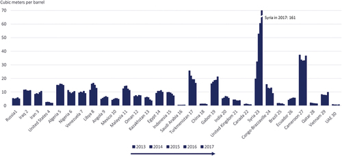
Under extractive political institutions, power is concentrated within a narrow group of elites who exploit resources from the rest of society (Robinson & Acemoglu, Citation2012). As a result, countries heavily reliant on fossil fuel production often experience poverty, corruption, and environmental pollution (Ebegbulem et al., Citation2013; World Bank, Citation2011). Despite the wealth generated from the sale of fossil fuels, these countries face significant income inequality and environmental degradation. In particular, the extraction of fossil fuels leads to the release of harmful emissions, such as flaring and gas emissions, contributing to air pollution. illustrates the flaring intensity for the top 30 flaring countries between 2013 and 2017. Moreover, these countries exhibit higher Gini coefficients compared to others.Footnote2
Figure 1. Flaring intensity in top 30 flaring countries from 2013 to 2017 (Global Gas Flaring Reduction Partnership). The values were ranked by 2017 flaring volume. The unit is cubic meters gas flared per barrel of oil produced. Global average intensity was 4.8 m3/bbl in 2017.
Fossil fuels are non-renewable energy resources formed through the high heat and pressure acting on the remains of animals or plants buried underground. The primary types of fossil fuels include coal, oil, and natural gas. Accordingly, fossil fuel rent encompasses coal rents, oil rents, and natural gas rents. Fossil fuel rents are defined as the difference between the global market value of coal, oil, and natural gas and the total costs associated with their production (World Bank, Citation2011). In the field of environmental and natural resource economics, rent refers to the marginal user cost, representing the present value of foregone opportunities when resources are scarce (Tietenberg & Lewis, Citation2018). Thus, fossil fuel rent can be viewed as a form of royalty, where the marginal user cost of fossil fuel equals the price of the fossil fuel minus the marginal extraction cost (Daly & Farley, Citation2011).
3. Theoretical model
The model proposes the validity for modified carbon curse theory which shows income inequality contribute to drive the higher carbon intensity in countries with higher dependence on fuel rents. To provide the analytical framework for the relationship fossil fuel resources, income inequality and carbon intensity, the model modified Smulder’s environmental endogenous growth model (1999).
Let be an index of total natural resources as a proxy for environmental quality, and the model assumes an accumulation process of natural resources two different flows. First, a stock of natural resource regenerates itself by exponential growth at an intrinsic rate
, where
is the growth rate of the renewable resources. Second, the stock of natural resource is depleted gradually by the aggregate extraction rate
which involves any economic activity that destroyed resources (i.e. fossil fuel resources) from nature. The extraction rate can be get
. Combining the two flows, we obtain the law of motion for total natural resources
, as
Consider the following Cobb-Douglas production function describing a closed and competitive economy with two state variables. Each firm produces output and aggregating over firms to take the form as follows
where and
are the stock of physical capital and utilized (destroyed or harvested) natural resource, respectively. Aggregate stock of natural resources
follows decreasing returns to scale when the physical and natural capital accumulation increases in production process, and
determinants the weight of positive external effect.
is equal
because this economy assume that aggregate output is produced from non-renewable natural resources such that
. This reflects a positive externality from extracted and used in non-renewable resources.
represents productive externalities by individual firms which is defined average level of the physical capital stock
:
In the symmetric equilibrium, so that all firm’s actions are the same. Therefore, we rewrite the production function are given by
and we obtain,
and
.
The economy is populated by many identical and infinitely-lived households and population is denoted by . The utility function for representative household’s consumption
is
where is the elasticity of substitution in consumption, for
and
and
is the subjective discount rate,
.The stock of physical capital constraint faced by the representative household is
. For the simplicity in calculation, the physical capital accumulation is assumed to be no depreciation in the model.
The utility function of households that depends on individual consumption and the budget constraint on the physical capital accumulation are
In this economy, individual households faced control over her consumption and capital allocation. The current value Hamiltonian for optimization problem is
At the steady state level, the growth rate grows along a balanced growth path at the same rate, which leads to and
. The growth rate
is
. Then, we can note that
, setting
and
where denote by
, the ratio of average capital to the capital owned by individual household
or the relative physical capital in generating the aggregate physical capital of the economy. Therefore,
determine the income inequality path of this economy.
Under the symmetric equilibrium condition and
that can be change to the aggregate level, and we can drive that there exists a relationship between the income inequality and natural resources dependence on extraction rate extraction rate e
The extraction rate depends on the ratio and the utilized natural resources. The ratio
can be seen as the extraction rate relevant income inequality in this economy. In fact, the higher income inequality, and the biggest dependence on destroyed natural capital, the higher extraction rate.
To derive a balanced growth path, the variable transformed consumption per unit of physical capital,
, and re-express aggregate equilibrium conditions as the following the optimal growth path of the economy using three differential equations:
Assume that the economy is in a steady state balanced growth equilibrium ( that satisfy the condition
It is possible to derive the steady states level for resource utilization,
along a unique balance growth path. This in turn leads to the steady of
, to be determined, as both are function of
.
If the economy is on a balanced growth path, we have to impose
represents the scale effect of production on utilized natural resources, thus, the growth rate of a balanced growth path is positively related to the steady-state level of utilized natural resources. That is, higher destroyed natural resources will raise with a higher extraction rate, economic growth through physical capital accelerates.
4. Data
The study utilized a panel data set consisting of 137 countries, which were divided into three income groupsFootnote3: 44 high-income countries, 41 middle-income countries, and 52 low-income countries. The data covered the period from 1980 to 2014. Table provides descriptions of the variables used in the study and presents summary statistics.Footnote4
Table 1. Data description and summary statistics
The dependent variable in the analysis is CO2 emissions per GDP, which measures carbon intensity. Carbon intensity represents the rate of CO2 emissions in relation to the intensity of economic activity. It captures variations in fuel consumption patterns across different industrial sectors. It is important to control for economic levels because carbon emissions are closely linked to the scale of economic activity. Therefore, CO2 emissions per GDP indicates the economic production value associated with each country’s CO2 emissions. A lower carbon intensity value signifies lower CO2 emissions relative to the size of the economy, indicating greater energy efficiency. In general, high-income countries tend to exhibit improved energy productivity, resulting in lower carbon intensity in their GDP (Fankhauser & Jotzo, Citation2018). On the other hand, low-income countries often have lower carbon intensity due to their lower level of economic activity compared to other income groups. This is because many individuals in low-income countries lack access to electricity or fossil fuels (Pachauri et al., Citation2013). Additionally, middle-income countries with abundant fossil fuel resources and high economic growth rates typically display higher carbon intensity compared to other income groups (Manley et al., Citation2017).
5. Empirical strategies
In this paper, we augment the carbon curse theory by exploring the causal relationships among variables related to income groups. Our goal is to understand the role that an economy dependent on fossil fuel rents may play in shaping income inequality and carbon intensity levels across countries.
5.1. Panel Granger causality
The panel Granger causality investigates the causal relationship between the variables in a time series. Granger causality was developed by Granger (Citation1969) to analyze the causal relationship between time series data. To determine the panel Granger causality, we consider a panel VAR model. This empirical study explores the relationships among carbon intensity, income inequality, and oil-dependency of countries. We consider a panel VAR with ordered panel-specific fixed effects, represented by the following linear equation:
The model under consideration can be expression as a lagged order panel VAR model:
The data stability of each variable is first checked using the panel unit root test. Further, we consider the Granger causality among oil rents, income inequality, and carbon intensity, by income group. If necessary, we conduct a panel cointegration test to confirm the long-term stable relationship between the three variables. If the data are stationary, the test is performed using the level values of variables. However, if the variables are non-stationary, the test is performed using first differences. The panel Granger causality is shown in the following model:
This can be used to test whether the independent variables affect the dependent ones. The null hypothesis is given as follows:
If is rejected, it can be concluded that causality between
to
exists in EquationEquation 24
(24)
(24) . Furthermore, if
is rejected, causality between
to
exists in EquationEquation 24
(24)
(24) . The null hypothesis in EquationEquation 24
(24)
(24) shows whether
and
are causally correlated to
. The variables are interchanged to test for causality in the other direction. Therefore, the basic idea of Granger causality is that a Granger variable
causes
, if past values of
can explain
.
5.2. Panel error correction model
If the data have a unit root, the time series are non-stationary. Thus, we estimate the model using the panel error correction model (PECM). The unit root test of panel data for countries and
periods can be represented as follows:
where denotes carbon intensity or other explanatory variables and
is the error term. The null hypothesis states that, if
, then the null hypothesis is rejected, and the series is considered stationary.
If the null hypothesis of the unit root is not rejected, the variables are non-stationary. Thus, we test the cointegration relationship, which indicates that two or more dependent variables are related in the long run. The equation can be expressed as follows:
where is the cointegration vector and
determines the speed at which the system readjusts its equilibrium relationship with the error correction term
after experiencing a sudden shock. If
is less than 0, the cointegration relationship exists, whereas the relationship does not establish when
is equal to 0 (Persyn & Westerlund, Citation2008). Additionally, a long-run relationship exists when the error term is stationary, although the dependent and independent variables are non-stationary.
indicates the short-term effect of independent variables on carbon intensity.
6. Results
6.1. Carbon intensity trajectory
visually presents the carbon intensity trajectory for each income group. The y-axis represents the annual growth rate of carbon intensity from 1996 to 2014,Footnote5 while the x-axis represents the log of the average Gini coefficient during the same period. In each figure, the colored circles indicate a higher share of oil rents as a percentage of GDP, with larger circles indicating greater dependence on oil rents. Following the categorization by Friedrichs and Inderwildi (Citation2013), the countries in are divided into three categories: emissions intensification (red), emissions increase (yellow), and emissions reduction (green). However, this study redefines the graph by examining the change in carbon intensity caused by income inequality.
Figure 2. The carbon intensity trajectory by income group.
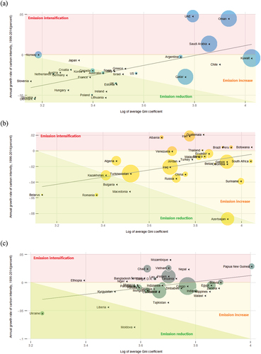
The red-shaded areas represent countries that have experienced the intensification of carbon intensity under high levels of income inequality, which can be associated with a greater share of oil rents in the economy. This pattern is particularly noticeable among high-income countries with a high dependency on oil rents. Countries with lower levels of oil rents are located in the lower left area of the graph, while countries highly dependent on oil rents, such as Oman, Saudi Arabia, and the UAE, have higher levels of income inequality and follow more carbon-intensive pathways due to the concentration of wealth in the hands of a few.
The yellow-shaded areas depict countries that have managed to reduce their carbon intensity, but their absolute carbon emissions are still increasing under high income inequality. These countries include China, Qatar, Russia, the US, and other oil-rich nations.
The green-shaded areas represent countries that have achieved high decarbonization alongside low levels of income inequality. This phenomenon can be attributed to two factors. First, these countries have made significant improvements in energy efficiency, leading to cleaner production processes. Additionally, they already had well-developed economies, which allowed them to raise living standards through economic growth and reduce income inequality. When wealth distribution becomes more equitable, it becomes easier to invest in carbon emission reduction. This trend is particularly prominent in European countries with strong environmental regulations. Second, countries undergoing economic reform, such as the EIT countries,Footnote6 exhibit a hockey-stick curve trend (Huang et al., Citation2008). Initially, they experience a rapid increase in emissions due to oil consumption for economic development. However, they are now making efforts to reduce their emissions by increasing the production and consumption of renewable energy.Footnote7 These countries have experienced fluctuations in emissions, with a quick fall followed by a rebound, which has led to economic instability. Additionally, the increase in emissions has dampened energy supply and availability, resulting in low levels of economic growth. Furthermore, these countries tend to have lower income inequality because they have not completely abandoned their socialist regimes.
In Figure , which focuses on high-income countries, it is evident that most of them have managed to decarbonize under lower levels of income inequality. These countries, with the exception of Norway, are not heavily dependent on oil rents. Norway, being a developed economy with access to advanced technology, shows a positive annual growth rate for carbon intensity amounting to 0.022%, despite its low Gini coefficient. The countries rich in oil and high in oil rents are located in the lower left area of the graph, indicating a higher level of emissions resulting from oil extraction. Certain high-income countries such as the UAE, Oman, and Saudi Arabia follow a different pathway, experiencing a quicker increase in carbon intensity under higher levels of income inequality and high oil rents.
Figure presents the data for middle-income countries. Countries with higher income inequality also exhibit a high annual growth rate of carbon intensity. At this income level, most countries are rich in oil rents and fall into the yellow-shaded areas, indicating that their absolute CO2 emissions are increasing as they prioritize economic growth for national development. The economic structures of countries such as Iran, Iraq, and Turkmenistan heavily rely on the oil production and extraction industry, which leads to high emissions and higher income inequality.
Figure shows the results for low-income countries. In these countries, the annual growth rate of carbon intensity has been increasing, and the Gini coefficient is concentrated in the range of 3.6–3.8. Low-income countries with a high dependence on oil rents are mostly concentrated in the red- and yellow-shaded areas, indicating that oil availability and extraction for economic development have not translated into energy efficiency in these economies.
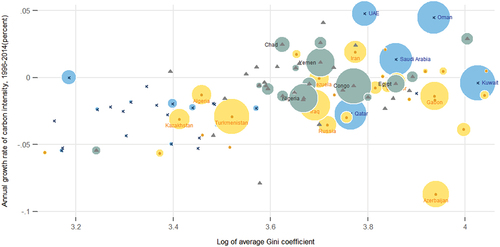
Appendix Figure provides the combined graph for all income groups. The graphs suggest the dependence of oil rents may contribute to the high levels of carbon intensity in countries facing unequal income distribution.
6.2. Panel unit root test and panel cointegration test
Before estimating the PECM, we conducted panel unit root tests to examine the time series properties of the variables. We employed three types of panel unit root tests: IPS, Fisher ADF, and Fisher PP tests (Im et al., Citation2003; Maddala & Wu, Citation1999). These tests are crucial as non-stationary variables (those possessing a unit root) can lead to spurious regression results when analyzing fixed effects among countries (Dickey et al., Citation1986; Newbold & Granger, Citation1974). To address this issue, we further examined the existence of a cointegration relationship between carbon intensity and the dependent variables. If the variables were found to be cointegrated, we proceeded with the estimation of the error correction model.
Table displays the results of the panel unit root tests for each income group. In the high-income group, the series of logarithmic CI (carbon intensity) appeared to have a unit root, but all series became stationary when differenced once. For the upper middle-income group, both logarithmic CI and GINI showed evidence of a unit root, but became stationary when differenced once. The GINI coefficient was non-stationary at all levels, but stationary at the first difference for the upper middle- and low-income groups.
Table 2. Results of panel unit root test
The panel vector error correction model (VECM) is utilized to analyze the long-run relationships between the variables, while the panel vector autoregression (VAR) is employed when cointegration is absent. To determine the presence of cointegration, we conducted unit root tests on the variables, which confirmed that all income groups exhibited stationarity in I(1).
We further examined the panel cointegration relationship between carbon intensity, income inequality, and oil rents using the Pedroni tests.Footnote8 Table presents the results of these tests. Under the null hypothesis of no cointegration in non-stationary heterogeneous panels , the test statistics are distributed (0, 1) and tend to diverge into negative infinity panels (Neal, Citation2014). In this study, we employed the Panel ADF and PP cointegration tests. The results of the Pedroni test indicate the presence of panel cointegration at a significance level of 1% for all income groups.
Table 3. Results of panel cointegration test
6.3. Panel Granger causality
The panel Granger causality test was conducted to determine the direction of the causal relationship between carbon intensity and its determinants. Before conducting the test, the stability condition was assessed by calculating the absolute values of each eigenvalue of the estimated model. The lag length selection criteria used was Schwarz’s information criterion (SIC), with a maximum lag of 1 considered for all estimated models. The stability condition is satisfied when all absolute values in the companion matrix are strictly less than 1 (Hamilton, Citation2020; Lütkepohl, Citation2005).
The results of the Granger causality test are presented in Table , and provides a summary of the Granger causality relationships. For high-income countries, panel causal relationships were found between income inequality, carbon intensity, and oil rents. These relationships were bilateral, indicating a Granger causality relationship [oil rents → income inequality → carbon intensity]. Similarly, for middle-income countries, a bidirectional causal relationship was observed between oil rents and income inequality, leading to a Granger causality relationship [oil rents → income inequality → carbon intensity]. In the case of low-income countries, a bilateral causal relationship existed between income inequality and carbon intensity, and a one-way causality was identified [oil rents → income inequality → carbon intensity], with oil rents directly affecting carbon intensity.
Figure 3. Granger causality relationship.
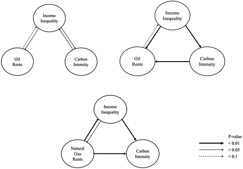
Table 4. Results of Granger causality test by income group
The results of the causal relationships support the hypotheses presented in this study and align with the evidence of the carbon trajectory. Based on the Granger causality relationships, the empirical findings suggest that variations in the share of oil rents in GDP influence the level of income inequality, which, in turn, impacts the carbon intensity of GDP for all income groups.
6.4. Panel error correction model
Given the evidence of panel cointegration, the long-run relationships among carbon intensity, income inequality, and fossil fuel rents can be further estimated by applying the Pedroni test. Additionally, the Granger causality is useful in identifying the cause-effect relationship with constant conjunctions. However, it is limited to the illustration of significant correlations between variables. Therefore, we estimate the model using the PECM to provide the relationship among carbon intensity, income inequality, and oil rents by estimating short- and long-run effects.
According to the empirical results, variables of lagged first-difference and lagged variables imply short-term and a long-term effects on the dependent variable. The interpretation of the coefficients in the PECM is based on the sign of the Granger causality, which indicates the presence of endogenous variables (Greene, Citation2003). The results are summarized in Tables . The PECM estimation indicates the correlation between the three variables by estimated models.
Table 5. Panel error correction model for high-income countries
Table 6. Panel error correction model for middle-income countries
Table 7. Panel error correction model for low-income countries
The results for high-income countries are presented in Table . The impact of income inequality on carbon intensity is positive in the short run and changes to negative in the long run. The oil rents are positively related to income inequality in the short run. The results also provide the error correction terms, which are significantly negative across all models. The variable of the error correction term determines the speed at which a dependent variable returns to equilibrium after the independent variables’ changes. If the coefficient of error correction term is significantly negative, we expect the dependent variable to respond significantly to the negative deviation from the long-run relationship.
The results for the middle-income countries are presented in Table . The results show that the impact of income inequality on carbon intensity is negative in the short run and changes to positive in the long run; however, it is insignificant. The oil rents are positively related to income inequality in the short run, whereas the carbon intensity has a negative impact on income inequality. The error correction terms have a significantly negative effect in each model.
Table displays the results of the low-income countries. The income inequality is negatively related to carbon intensity in the short run. The oil rents, as a share of GDP, have a positive effect in the long run. The income inequality and oil rents have a positive impact on each other in the long run. The error correction terms are significantly negative across all models.
The estimation of the PECM yields several noteworthy results. Firstly, the findings indicate a significantly positive relationship between income inequality and oil rent across all income groups. Oil rents contribute to an increase in income inequality within a country. However, this effect diminishes in the short run as the share of oil rents in GDP increases, particularly for high- and middle-income countries. Conversely, in low-income countries, the short-run impact of oil rents is negligible, but their effects become apparent over time. These findings suggest that economies heavily reliant on oil rents can have a detrimental effect on income distribution, especially when the share of oil rents in GDP rises. Low-income countries are particularly vulnerable to this effect.
Secondly, the impact of income inequality on carbon intensity varies depending on the income level. Initially, an increase in income inequality leads to higher carbon intensity, indicating a positive relationship. However, as economic growth is achieved, income inequality gradually contributes to a reduction in carbon emission levels in high-income countries. In contrast, middle- and low-income countries exhibit an inverse effect, suggesting that income inequality leads to increased carbon emissions in these income groups.
7. Conclusion
This study aims to investigate the relationship between extractivism, income inequality, and carbon intensity across 134 countries. The research model in this article is closely aligned with the framework proposed by Friedrichs and Inderwildi (Citation2013), but it introduces a novel aspect by incorporating income inequality into the augmented carbon curse theory. The primary objective of the study is to examine how the interplay between fossil fuel endowment and income inequality affects carbon emissions in a country’s economic output, taking into account different income levels. Given that CO2 emissions are influenced by various factors related to economic activities, the article specifically explores the connection between income inequality and CO2 emissions in countries that heavily rely on fossil fuel production.
The analysis of the carbon intensity trajectory for different income groups provides support for the notion that countries heavily reliant on fossil fuel rents tend to exhibit higher levels of both income inequality and carbon intensity. The empirical findings demonstrate that larger amounts of fossil fuel rents have an impact on the relationship between income inequality and carbon intensity within a country’s GDP. Economies that rely on fossil fuel rents often display a more unequal distribution of income and follow a more carbon-intensive developmental path. The panel causality test reveals the presence of unidirectional causal relationships among oil rents, income inequality, and carbon intensity, specifically from oil rents to income inequality and then to carbon intensity [oil rents → income inequality → carbon intensity].
In the short run, higher levels of fossil fuel rents contribute to an increase in income inequality, and higher income inequality, in turn, leads to greater carbon intensity in high-income countries. However, middle- and low-income countries experience a decrease in carbon intensity despite higher income inequality. In the long run, the short-term effect of fossil fuel rents on income inequality persists, but higher income inequality results in a reduction of carbon intensity in high-income countries. The impact of income inequality on carbon intensity is not observed in middle- and low-income countries. Overall, the evidence suggests that the abundance of oil resources plays a role in determining the distribution of rents and contributes to income inequality. Consequently, an economic structure heavily dependent on oil has implications for carbon intensity. Therefore, when considering a country’s income distribution, it is crucial to take into account carbon-intensive pathways as they are linked to the rents derived from natural resources.
Indeed, the results suggest that addressing income distribution policies and adopting effective natural resource management strategies are crucial components of a country’s carbon neutral strategy. The findings indicate that countries with a high dependence on fossil fuel rents tend to exhibit higher levels of income inequality and carbon intensity. This highlights the need for policies that aim to promote a more equitable distribution of income and wealth, while also transitioning towards cleaner and more sustainable energy sources.
By integrating income distribution policies into carbon neutral strategies, countries can work towards reducing income inequality and ensuring that the benefits of sustainable development are shared more equally among the population. This may involve implementing measures such as progressive taxation, social welfare programs, and targeted investments in education and skill development to create more opportunities for all segments of society.
Additionally, effective natural resource management is essential to mitigate the environmental impact of carbon-intensive activities. Countries can pursue strategies that prioritize the sustainable extraction and use of natural resources, including the implementation of regulations, incentives, and technological advancements to promote cleaner production processes and energy efficiency. This can contribute to a more balanced and environmentally sustainable economic development path.
By incorporating income distribution policies and sustainable natural resource management practices into their carbon neutral strategies, countries can work towards achieving both environmental and social goals. This integrated approach can help create a more inclusive and resilient economy that addresses income inequality while transitioning towards a low-carbon and sustainable future.
Correction
This article has been corrected with minor changes. These changes do not impact the academic content of the article.
Disclosure statement
No potential conflict of interest was reported by the author(s).
Data availability statement
The author confirms that all data generated or analyzed during this study are included in this published article.
Notes
1. Fugitive emission refers to pollutants released into the air from industry operation. The major part of the fugitive emissions is emitted as CO2 mainly from flaring in upstream oil and gas production. The sectors contributing to fugitive emissions include extraction, handling, storage, transmissions, and distribution of solids, liquids, and gaseous fuels, and from flaring and venting (Plejdrup et al., 2015).
2. Global average Gini coefficient is 38.1, the average of top 30 flaring countries is 40.4 (ICRG, 2017).
3. According to the World Bank’s national classification by income level, high income countries are defined as those with a GNI per capita of $12,235 or more; upper-middle income countries have a GNI per capita between $3,956 and $12,235; lower-middle income countries have a GNI per capita between $1,006 and $3,955; lower-middle income countries have a GNI per capita of $ 1,005 or less (World bank, 2017b).
4. CO2 emissions per GDP and oil rents data were obtain from World Bank database. GINI data was obtained from the Standardized World Income Inequality Database (SWIID), and it specifies that for certain countries categorized as middle- and low-income countries, the available data only goes up until 2014.
5. In order to calculate the growth rate, it is necessary to base the year for which all data for the country exist, and in this case, it was calculated based on 1996.
6. EIT refers to countries with “economies in transition,” that is, Belarus, Bulgaria, Croatia, Czech Republic, Estonia, Hungary, Latvia, Lithuania, Poland, Romania, Russia, Slovak Republic, Slovenia, and Ukraine, among the Kyoto Protocol Annex I counties.
7. Bulgaria has already achieved the EU targets for production and consumption of electricity from renewable sources, set in the Europe 2020 strategy. In 2012, Bulgaria’s share of renewables for final energy consumption stood at 16.3%, against a target of 16%. Estonia was the first Member State to reach its 2020 targets, which was 25% in 2011 (Eurostat, 2014).
8. In general, cross-sectional dependence between panel groups can occur in panel analysis. Westerlund (2007) present a panel cointegration test method that eliminates cross-sectional interdependence using a panel model. As a result of Pesaran’s CD test, there is evidence suggesting the presence of cross-sectional dependence, therefore, we use panel stationarity test: Fisher-ADF, Fisher-PP.
References
- Bergner, P. (2016). “Income inequality and natural resources.” https://lup.lub.lu.se/student-papers/search/publication/8890838
- Daly, H. E., & Farley, J. (2011). Ecological economics: Principles and applications (2nd ed). Island Press.
- Dickey, D. A., Bell, W. R., & Miller, R. B. (1986). Unit roots in time series models: Tests and implications. The American Statistician, 40(1), 12–20. https://doi.org/10.1080/00031305.1986.10475349
- Dudley, B. (2018). BP statistical review of world energy 2018. Energy economic, Centre for energy economics research and policy. British Petroleum., Available via https://www.bp.com/en/global/corporate/energy-economics/statistical-reviewof-world-energy/electricity.html5
- Ebegbulem, J. C., Ekpe, D., & Adejumo, T. O. (2013). Oil exploration and poverty in the Niger Delta Region of Nigeria: A critical analysis. International Journal of Business & Social Science, 4(3), 279–287. https://ijbssnet.com/journals/Vol_4_No_3_March_2013/30.pdf
- Eurostat. (2014). The EU in the world 2014. https://ec.europa.eu/eurostat/documents/3217494/5786625/KS-EX-14-001-EN.PDF
- Fankhauser, S., & Jotzo, F. (2018). Economic growth and development with low‐carbon energy. Wiley Interdisciplinary Reviews: Climate Change, 9(1), e495. https://doi.org/10.1002/wcc.495
- Friedrichs, J., & Inderwildi, O. R. (2013). The carbon curse: Are fuel rich countries doomed to high CO2 Intensities? Energy Policy, 62, 1356–1365. https://doi.org/10.1016/j.enpol.2013.07.076
- Fum, R. M., & Hodler, R. (2010). Natural resources and income inequality: The role of ethnic divisions. Economics Letters, 107(3), 360–363. https://doi.org/10.1016/j.econlet.2010.03.008
- Gavenas, E., Rosendahl, K. E., & Skjerpen, T. (2015). CO2-Emissions from Norwegian oil and gas extraction. Energy, 90, 1956–1966. https://doi.org/10.1016/j.energy.2015.07.025
- GGFR. (2017). GGFR flaring data. https://www.worldbank.org/en/programs/gasflaringreduction/global-flaring-data
- Goderis, B., & Malone, S. W. (2011). Natural resource booms and inequality: Theory and evidence. Scandinavian Journal of Economics, 113(2), 388–417. https://doi.org/10.1111/j.1467-9442.2011.01659.x
- Granger, C. W. (1969). Investigating causal relations by econometric models and cross-spectral methods. Econometrica: Journal of the Econometric Society, 37(3), 424–438. https://doi.org/10.2307/1912791
- Greene, W. H. (2003). Econometric analysis. Pearson Education India.
- Griffiths, S. (2017). A review and assessment of energy policy in the middle east and north Africa Region. Energy Policy, 102, 249–269. https://doi.org/10.1016/j.enpol.2016.12.023
- Gylfason, T., & Zoega, G. (2003). Inequality and economic growth: Do natural resources matter? Inequality and Growth: Theory and Policy Implications, 1, 255. https://doi.org/10.2139/ssrn.316620
- Hamilton, J. D. (2020). Time series analysis. Princeton university press.
- Huang, W. M., Lee, G. W., & Wu, C. C. (2008). GHG emissions, GDP growth and the Kyoto protocol: A revisit of environmental Kuznets curve hypothesis. Energy Policy, 36(1), 239–247. https://doi.org/10.1016/j.enpol.2007.08.035
- ICRG. (2017). International country risk guide researchers dataset. 2017 version. 2017 version. https://dataverse.har¬vard.edu/dataset.xhtml?persistentId=hdl:1902.1/21446
- IEA. (2017). CO2 emissions from fuel combustion 2017. https://www.oecd-ilibrary.org/energy/co2-emissions-from-fuel-combustion-2017_co2_fuel-2017-en.
- Im, K. S., Pesaran, M. H., & Shin, Y. (2003). Testing for unit roots in heterogeneous panels. Journal of Econometrics, 115(1), 53–74. https://doi.org/10.1016/S0304-4076/0300092-7
- Johnsson, F., Kjärstad, J., & Rootzén, J. (2019). The threat to climate change mitigation posed by the abundance of fossil fuels. Climate Policy, 19(2), 258–274. https://doi.org/10.1080/14693062.2018.1483885
- Kwakwa, P. A., Alhassan, H., & Adu, G. (2019). Effect of natural resources extraction on energy consumption and carbon dioxide emission in Ghana. International Journal of Energy Sector Management, 14(1), 20–39. https://doi.org/10.1108/IJESM-09-2018-0003
- Leamer, E. E., Maul, H., Rodriguez, S., & Schott, P. K. (1999). Does natural resource abundance increase Latin American income inequality? Journal of Development Economics, 59(1), 3–42. https://doi.org/10.1016/S0304-38789900004-8
- Li, R., Wang, Q., Liu, Y., & Jiang, R. (2021). Per-capita carbon emissions in 147 countries: The effect of economic, energy, social, and trade structural changes. Sustainable Production and Consumption, 27, 1149–1164. https://doi.org/10.1016/j.spc.2021.02.031
- Lütkepohl, H. (2005). New introduction to multiple time series analysis. Springer Science & Business Media. https://doi.org/10.1007/978-3-540-27752-1
- Maddala, G. S., & Wu, S. (1999). A comparative study of unit root tests with panel data and a new simple test. Oxford Bulletin of Economics and Statistics, 61(S1), 631–652. https://doi.org/10.1111/1468-0084.0610s1631
- Manley, D., Cust, J. F., & Cecchinato, G. 2017. “Stranded nations? The climate policy implications for fossil fuel-rich developing countries.” The Climate Policy Implications for Fossil Fuel-Rich Developing Countries (February 1, 2017). OxCarre Policy Paper 34.
- Neal, T. (2014). Panel cointegration analysis with Xtpedroni. The Stata Journal, 14(3), 684–692. https://doi.org/10.1177/1536867X1401400312
- Newbold, P., & Granger, C. W. (1974). Experience with forecasting univariate time series and the combination of forecasts. Journal of the Royal Statistical Society Series A (General), 137(2), 131. https://doi.org/10.2307/2344546
- Pachauri, S., van Ruijven, B. J., Nagai, Y., Riahi, K., van Vuuren, D. P., Brew-Hammond, A., & Nakicenovic, N. (2013). Pathways to achieve universal household access to modern energy by 2030. Environmental Research Letters, 8(2), 024015. https://doi.org/10.1088/1748-9326/8/2/024015
- Parcero, O. J., & Papyrakis, E. (2016). Income Inequality and the oil resource curse. Resource and Energy Economics, 45, 159–177. https://doi.org/10.1016/j.reseneeco.2016.06.001
- Persyn, D., & Westerlund, J. (2008). Error-correction–based cointegration tests for panel data. The STATA Journal, 8(2), 232–241. https://doi.org/10.1177/1536867X0800800205
- Plejdrup, M. S., Nielsen, O. K., & Nielsen, M. (2015). Emission inventory for fugitive emissions from fuel in Denmark. Aarhus University, Department of Environmental Science.
- Robinson, J. A., & Acemoglu, D. (2012). Why nations fail: The origins of power, prosperity and poverty. Profile.
- Ross, A. (2007). Multiple identities and education for active citizenship. British Journal of Educational Studies, 55(3), 286–303. https://doi.org/10.1111/j.1467-8527.2007.00380.x
- Tietenberg, T., & Lewis, L. (2018). Environmental and natural resource economics. Routledge.
- UNFCCC. (2012). Kuwait’s initial national communication under the United Nations framework convention on climate change. https://unfccc.int/resource/docs/natc/kwtnc1.pdf
- UNFCCC. (2016). Third national communication of the kingdom of Saudi Arabia under the United Nations Framework convention on climate change. https://unfccc.int/files/national_reports/non-annex_i_natcom/application/pdf/saudi_arabia_nc3_22_dec_2016.pdf
- Wang, Q., Wang, L., & Li, R. (2023). Trade protectionism jeopardizes carbon neutrality–decoupling and breakpoints roles of trade openness. Sustainable Production and Consumption, 35, 201–215. https://doi.org/10.1016/j.spc.2022.08.034
- Wang, Q., Yang, T., & Li, R. (2023). Does income inequality reshape the environmental Kuznets curve (EKC) hypothesis? A nonlinear panel data analysis. Environmental Research, 216, 114575. https://doi.org/10.1016/j.envres.2022.114575
- Wang, Q., Zhang, F., & Li, R. (2023). Revisiting the environmental kuznets curve hypothesis in 208 counties: The roles of trade openness, human capital, renewable energy and natural resource rent. Environmental Research, 216, 114637. https://doi.org/10.1016/j.envres.2022.114637
- Westerlund, J. (2007). Testing for error correction in panel data. Oxford Bulletin of Economics and Statistics, 69(6), 709–748. https://doi.org/10.1111/j.1468-0084.2007.00477.x
- World Bank. (2011). The changing wealth of nations: Measuring sustainable development in the new millennium. World Bank Group Publications.
- World Bank. (2017a). New country classifications by income level: 2017–2018
- World Bank. (2017b). New country classifications by income level: 2017–2018. https://blogs.worldbank.org/opendata/new-country-classifications-income-level-2017-2018
- World Bank. 2018. World development indicators. https://databank.worldbank.org/source/worldbank.org/source/world-development-indicators
- Zhu, Z. S., Liao, H., Cao, H. S., Wang, L., Wei, Y. M., & Yan, J. (2014). The differences of carbon intensity reduction rate across 89 countries in recent three decades. Applied Energy, 113, 808–815. https://doi.org/10.1016/j.apenergy.2013.07.062
Appendix
Table A1. Fossil fuel abundance and rents as a share of GDP in 2014
Figure 41. The relationship between Gini and annual growth of carbon intensity for all countries. The colored circles indicate the share of oil rents as a share of GDP.