Inter-sectoral linkages and economic growth in Uganda: A SAM-based multiplier model analysis

Abstract

Sectors are the engines of economic growth in any economy making inter-sectoral linkages the most significant target for development practitioners and policymakers. This study examines and ascertains the magnitude of production and consumption inter-sectoral linkages in Uganda’s economy. Secondary data from 2009/10 and 2016/17 Uganda Social Accounting Matrices (SAMs) is analyzed based on the multiplier model. A buttress of robust checks including a Vector Error Correction Model (VECM) is adopted for validation purposes using a longer time series from 1980 to 2020. The study found that a one million income injection across sectors has a larger multiplier effect (in terms of output, GDP, income, and consumption) than the service sector followed by agriculture and then the industrial sector. Despite the higher multiplier effects of the services sector, its contribution to employment is limited. A large amount of labor is trapped in the low-paying subsistence agricultural sector. Therefore, the government should implement policies that supplement rapid services sector growth with strategies that attract and utilize excess labor in the agricultural sector. Results also indicate that the services sector prematurely emerged as the driver of economic growth before the economy was fully industrialized. Government should formulate industrial sector catch-up policies to rebalance its development agenda. To accomplish this, proportionately more funding should be allocated to the industrial sector. Lastly, sectoral multiplier effects projections and forecasts should be incorporated into the National Development Plans, Budgeting Frameworks, and forecasts.

Keywords:

• inter-sectoral linkages
• multiplier model
• social accounting matrix
• VECM

JEL Classification:

• C01
• O41
• J21
• C22
• E16

PUBLIC INTEREST STATEMENT

In this paper, we investigate the intersectoral linkages in Uganda’s economy. we consider sectors as the units of analysis. Sectors of an economy are the engines that spur economic growth and development. They create goods and provide employment, and tax revenue to the government. This study examines and ascertains the magnitude of production and consumption inter-sectoral linkages in Uganda’s economy based on data from 2009/10 and 2016/17 SAMs analyzed using the multiplier model. A buttress of robust checks including a Vector Error Correction Model (VECM) is adopted for validation purposes using a longer time series from 1980 to 2020. The findings of this study confirm that a one million income injection across sectors has a larger multiplier effect (in terms of output, GDP, income, and consumption) in the service sector followed by agriculture and then the industrial sector. A large amount of labor is trapped in the low-paying subsistence agricultural sector.

1. Introduction

Uganda like other developing countries has been experimenting with different development frameworks for a while but with limited success. It is argued that identifying the sector of the economy with a high growth impulse that can be nurtured to achieve economic transformation is an uphill task for these countries (Nguyen et al., 2022; Ogbonna et al., 2020). Uganda’s economy has recorded gradual structural changes in the agriculture, industry, and service sectors. The agricultural sector’s contribution to GDP dropped from over 50% in the 1990s to 20% in 2018/19, although the sector remains vital as it engages over 70% of the population (Nguyen et al., 2022; UBOS, 2019). In this context, a fascinating empirical question is to identify which sectors of the economy have the largest direct and indirect (i.e. production and consumption) linkages. In this case, production linkages are divided into forward and backward linkages according to (Breisinger et al., 2010).

Inter-sectoral linkages in an economy are sparked by exogenous demand-side shocks. The impact of such shocks is traced through their effect on investment, export demand, and government spending. This shock has both a direct and indirect effect on the economy, while the indirect effect is separated into consumption and production linkages. Further, production linkages are separated into forward and backward production linkages. Production linkages arise when sectoral production expands and provides more income to production factors and households. This income is then used to purchase additional goods and services. Jami (2006) says three factors determine the size of consumption linkages. That is to say the composition of the consumption basket, household income from factors of production, and the share of consumer goods supplied domestically. Haggblade et al. (2010) state unequivocally that consumption is responsible for 85 and 55% of multiplier effects in sub-Saharan Africa and Asia. This shows that consumption linkages far outpace production linkages in developing countries.

Theoretically, literature on the inter-sectoral linkages is examined based on the dual-economy model thanks to (Chenery, 1982; Feder, 1982; Lewis, 1954). This literature postulates a leader-follower relationship among sectors in an economy. According to this theory, the agriculture sector leads and provides raw materials and frees labor for the industrial sector. However, this model has been criticized for its rigidity (Gemmell et al., 1998, 2000). On the other hand, the empirical literature on this topic follows two strands. The first analysis is based on static models such as input-output, the social accounting matrix (SAM), and the more data-driven and complex computable general equilibrium (CGE) models (Breisinger et al., 2010; Punt, 2013; Pyatt & Round, 1985; Thurlow, 2008). The second follows econometric methods based on panel and time series data which introduce dynamism into the economic system (Bwire et al., 2016; Singh, 2015; Subramaniam & Reed, 2009; Varkey & Panda, 2018).

The purpose of this study is to broaden our understanding of intersectoral linkages in Uganda’s economy and its implied impact on economic growth in general. Previous studies on the sectoral linkages in Uganda are based on economic reports, sectoral performance surveys, and qualitative and case studies that lack empirical depth and quantitative rigor. Further, limited attention has been given to the analysis of production and consumption inter-sectoral linkages in the case of Uganda. Studies such as (Ggoobi et al., 2017; Muwonge et al., 2007; Shinyekwa et al., 2016) have reported contradictory results on sectoral linkages and structural transformation. Muwonge et al. (2007) for example find limited linkages between these informal and former sectors. The author pins this down to the economic disruptions of the early 1980s. Relatedly, Shinyekwa et al. (2016) analyzed the evolution of the industrial sector in Uganda and found limited intersectoral linkages of the industrial sector to other sectors. This was due to the premature early withdrawal of direct government intervention.

Empirically, the majority of the available studies have reported conflicting results regarding the direction and size of the impact. Besides most of these studies are sector-specific. For instance, Sastry et al. (2003) applied an input-out (IO) and simultaneous equation models in India and found that agriculture significantly impacted economic growth by influencing the demand linkages with other sectors. Similarly, in the United Kingdom, Gollin et al. (2002) investigated the role of the agricultural sector in development using a simple model and found that low productivity in the agricultural sector can indeed delay the onset of industrialization. This is a key finding that is synonymous with traditional development literature (Mlambo et al., 2019). Similarly, Subramaniam and Reed (2009) examined sectoral linkages in Poland and Romania, focusing mainly on how agriculture affects the rest of the economic sectors. The authors find that agriculture had a positive impact on all sectors in the two countries. In Uganda, Bwire et al. (2016) find evidence that infrastructural investment has strong growth linkages than both the industrial and the services sectors. Despite the wide application of non-econometric models (i.e. input-output (IO), SAM, and CGE), Singh (2015) has argued that these approaches are based on fixed prices and time-invariant technical coefficients.

We examine the magnitude of production and consumption inter-sectoral linkages using the SAM multiplier model and the VECM framework. Based on Uganda’s SAM 2009/10 and SAM 2016 and time series spanning 1980 to 2020. The results indicate that a one million income injection across sectors has a larger multiplier effect than the service sector. Agriculture comes next, followed by industry.

The significance of this study stems from the fact that there has not been much research carried out in Uganda to evaluate production and consumption inter-sectoral linkages. It is crucial to understand the flow of linkages among sectors in the economy in order to nurture sectors with higher effects on the economy (Nnyanzi et al., 2022). There no are clear linkages in Uganda’s context as regards to production and consumption linkages according to existing research (Shinyekwa et al., 2016). We attempt to fill this gap in this study. This study makes several contributions. Our study adds to the existing literature by documenting a finding that contradicts previous research (see Bwire et al. 2016). Additionally, our findings contribute to understanding sectoral growth multipliers, forecasts, and economic planning. From a practical standpoint, this study shows that well-implemented sectoral growth multiplier planning has the potential to result in long-term ripple growth effects throughout the economy.

As for the rest of this paper, it is organized as follows. Section 2 examines the literature on inter-sectoral linkages. In section 3, we describe the methodology and the data sources. A description of the study’s findings and a correlation matrix are presented in section 4. The findings and implications of the study are also discussed in this section. Section 5 discusses robustness checks. Section 6 contains the study’s conclusions

2. Literature on intersectoral linkages

2.1. Theoretical review

There is a plethora of theoretical literature that explains sectoral growth and inter-sectoral linkages in development economics. However, the most widely cited theory is the dual-economy model (Jorgenson, 1961; Lewis, 1954; Ranis & Fei, 1961). These studies are thoroughly discussed by Ruttan (1965). In this study, Ruttan (1965) argues that the dual-economy models were advanced to explain the relationship between the lagging traditional agricultural sectors and growing modern industrial sectors. Economic dualism as is popularly known in development economic discourse has two variants that emerged in the early 1950s, namely the static (i.e. sociological and enclave) dualism and dynamic dualism credited to the works of (Jorgenson, 1961; Lewis, 1954; Ranis & Fei, 1961). The static model assumes less interaction between the modern and traditional sectors in the economy, while the dynamic model emphasizes increased interaction between the two sectors (Amano, 1980; Ruttan, 1965). Out of all earlier theorizing, Lewis (1954) dual-economy model stands out and helped to bridge the divide between static and dynamic dualism, which has since formed the basis for the vast dual-economy literature. Broadly, the dual-economy models for developing countries were further categorized into classical and neoclassical (Jorgenson, 1961).

Generally, the linkages between the agricultural sector and the rest of the economy have been classified into Lewis linkages and Johnston-Mellor linkages (Barrett et al., 2010). Under the “Lewis” linkages”, the agricultural sector supplies the industrial sector with freed-up labor gained from the agricultural sector’s increased productivity. Lewis linkages operate largely through factor markets. Under the Lewis linkages, the economy will gain if low-productivity labor is transferred from rural-based sectors to urban-based sectors (Syrquin & Chenery, 1989). According to Chenery (1982) if the factor markets work perfectly, then the productivity gains from the structural adjustments will be few and saturated. On the other hand, the indirect “Johnston-Mellor linkages”, permit interaction in the input-output model between any two sectors to allow the agricultural sector to contribute to economic growth. The Johnston-Mellor linkages are supply-type linkages through which the agricultural sector supplies raw material, food, and market to the industrial sector, and also exports agro-produce to earn foreign exchange to aid in the importation of capital goods. Similar to Lewis linkages, the efficiency of factor markets determines how the agricultural sector’s contribution affects the economy.

According to Clement (2015), under economic duality both technologically advanced and primitive sectors co-exist. In this case, technology is adopted to extract resources in the presence of large subsistence production methods common in developing countries. The resource-abundant agriculture sector provides inputs to the resource constraint industrial sector. In other words, labor flows to the sector with higher wages. Conversely, considering the law of comparative advantages, the marginal productivity of labor in the industrial sector is higher than that of the agricultural sector, which will attract rural agricultural workers to migrate to urban industrial centers (Amano, 1980; Shumway, 1995). According to Gemmell (1982, 1998, 2000), sectoral linkages can be also analyzed in terms of both forward and backward linkages which are either positive or negative. For instance, an increase in agricultural output at lower levels of development will increase demand for nonagricultural goods (i.e. backward linkage). While increased expenditure on agricultural inputs from nonagricultural activities forms the forward linkages (Barrett et al., 2010).

Another version of the duality model is discussed by Baumol (1967). According to Baumol, the entire market output is produced by the progressive sector, while the stagnant sector produces no output. In this model, the stagnant sector faces boundless increasing per-unit cost which increases the demand for the progressive sector output. In return, the progressive sector attracts more and more labor in absence of substitutes from other sectors. In this simple model, the growth impacts of the stagnant sector are dominant which in Baumol’s view leads to the phenomenon known as the “cost disease of stagnant services”.

In contrast, under the perfect competition assumption, abnormal profits will attract more manufacturing firms to enter the market. This will increase demand for factors of production in the manufacturing sector thus shrinking the agricultural sector (Dabús & Delbianco, 2021; Kaur et al., 2009; Rashid, 2004). To be competitive in the market and to offset higher factor prices, the agricultural sector must increase the productivity of land and labor. To increase land productivity, agriculture must be mechanized and labor must be skilled. Through the provision of machines by the industrial sector and skilled labor by the services sector, the two sectors form positive (backward linkages) to the agricultural sector (Dabús & Delbianco, 2021). If the industry fails to provide the prerequisite technological advancement to agriculture, then this relationship will be detrimental instead to the agricultural sector, implying negative linkages. These interactions will continue until all three sectors attain equilibrium where the marginal product of resources is equal. At this point, the economy starts to experience growth because both average wage rates and the productivity of resources increases.

In summary, there is no single collective model that explains inter-sectoral linkages in an economy. Some authors support the most widely adopted dual-economy model (Lewis, 1954), while other studies support the leader-follower model. In this study, we explore both production and consumption linkages based on Social Accounting Multiplier (SAM) model.

2.2. Empirical literature

Empirically, two strands of analytical technique dominate the study of inter-sectoral linkages. First is the non-econometric methods which comprise the traditional input-output (IO), social accounting matrix (SAM), and the more complex and data-driven computable general equilibrium model (CGE) (Breisinger et al., 2010; Defourny & Thorbecke, 1984; Punt, 2013; Pyatt & Round, 1985; Round, 2005; Thurlow, 2008). Second, is the econometric strand which applies estimation techniques such as Vector Autoressuve models (VAR), Vector Error Correction models, and Autoregressive Distributed Lag (ARDL) models among others (Singh, 2015; Solanki et al., 2020; Subramaniam & Reed, 2009). Whereas national accounting techniques such as the SAMs have been around for the last 50 years, in Uganda, the first SAM was compiled in 2002. Later, the SAM 2009/10 and the Supply Use Table (SUT) were developed by the Uganda Bureau of Statistics (UBOS). In 2016 due to the emergence of new activities, the SAM and SUT 2016/17 were developed by the Ministry of Finance, Planning and Economic Development (MOFPED) and (UBOS), in partnership with the Victoria University’s Centre for policy studies (COPS) in Australia (Tran et al., 2019).

A few studies in Uganda have used of SAMs data and modeling frameworks to analyze sectoral linkages and economic growth. For instance, a study by Bwire et al. (2016) calibrated the SAM-based model to the Uganda SAM 2009/10 to investigate the impact of public and private investment shock on sectoral performance. The authors found that investment had a positive impact on growth in general. Varying by sector, the highest income multiplier effects are reported for infrastructural investment. In addition, the authors report excess capacity in the agricultural sector in terms of labor employment, with returns on capital investment exceeding returns from investment in labor by more than double, indicating that larger amounts of resources are trapped either unemployed or underemployed in the agricultural sector. These findings collaborate with those by Matovu (2000) who compared the welfare impacts of social spending on human capital and infrastructure spending based on the CGE model. His results indicated that social spending was more growth-enhancing in Uganda.

Relatedly, Randriamamonjy and Thurlow (2017) provided standardized techniques for constructing SAMs across economies in a nexus project. The authors demonstrated their procedure based on the 2013 Uganda SAMs. The intention of the nexus project in the construction of the SAM was to increase the traceability of data in the SAM to improve policy. On the other hand, Breisinger et al. (2010) provide a step-by-step construction of the SAM based on the Ghana SAM 2007. The author demonstrated the linkage between the circular flow of income and the SAM, identifying direct and indirect linkages, in their illustrations, indirect effects were decomposed into production and consumption linkages. While the production linkages were further categorized into forward and backward linkages. According the Breisinger et al. (2010), the strength of inter-sectoral linkages is weakened by leakages from the system such as taxes and imports.

Two studies that bring dynamism to SAM-based modeling are Llop Llop (2005) study in Spain and Jami (2006) study in Bangladesh. Llop Llop (2005) decomposes multipliers from two SAMs for 1990 and 1994 for the Catalan economy to reveal factors that lead to their variation over time. Based on both additive and multiplicative structural decomposition techniques, the author finds that a reduction in the structural coefficients of the model explains variability in the regional multipliers between the two periods. On the other hand, Jami (2006) developed the SAM 2000 for Bangladesh and finds that similar interventions have different income generation capacities for different income groups. Other notable and indicative studies in this field include (Defourny & Thorbecke, 1984; Phoofolo, 2018; Punt, 2013; Pyatt & Round, 1985; Round, 2005).

On the other hand, studies based on econometrics approaches have been revealing, for instance, Gemmell et al. (1998) in Malaysia examined the linkages between the agricultural, services, and industrial sectors. The authors found that in the short run, an increase in the manufacturing sector reduced output in the agricultural sector. While in the long run, agricultural output expanded as manufacturing output increased. Conversely, an increase in the services sector was associated with a reduction in agricultural output in both short and long-run scenarios. Their Granger causality results showed that both the services and manufacturing sectors weakly cause agricultural growth and the impact was unidirectional. The positive spillover effect of the manufacturing sector is consistent with neoclassical theoretical arguments. A study by Rashid (2004) in Pakistan examined growth linkages of the agricultural, industrial, and various components of the services sectors between (1971 to 2002). Based on OLS and Granger causality methods, the author found that both the industrial and the services sectors were more growth-stimulating for the agricultural sector.

In a Nigerian study, Onakoya (2013) examined the impact of the manufacturing, oil, and gas, and the services sector on the growth of the agricultural sector, based on the simultaneous equations macro-econometric model. The author found evidence for complex and multifaceted sectoral interdependencies. The authors found that capital flew from the agricultural sector towards manufacturing, oil and gas, and services in a unidirectional fashion. The author concluded that inter-sectoral relationships are not always beneficial for the agricultural and oil sectors in Nigeria. Similarly, Varkey and Panda (2018) examined the inter-sectoral linkages between agriculture, industry, and services among 15 Indian states. The authors found that the industrial and the services sectors had a positive and negative relationship with the agricultural sector respectively.

In a nutshell, the empirical literature above points to the compelling evidence for the existence of large sectoral interlinkages that are bi-direction, positive and negative. On the other hand, most of these studies except for Singh (2015) rely on the input-output (IO) technique to examine sectoral interlinkages, however, the IO models are based on fixed prices and time-invariant technical coefficients which are used in the technology matrix that forms the core of this approach. Time invariance implies the IO model provides a static snapshot of the sectoral linkages. Given this background, the present study employs a SAM-based multiplier model complemented by time series techniques to address time invariance problem in the analysis.

3. Methodology and data sources

3.1. Conceptual framework

One way of depicting the inter-sectoral linkages in an economy is through the circular flow diagram which shows inter-relationships between different sectors and institutions in an economy. According to Breisinger et al. (2010), the circular flow can be operationalized by a social accounting matrix (SAM). Through this representation, the production activities are supported by both factor and commodity markets. The factor markets provide factors of production while the commodity markets provide goods and services, supported by imports. The produced goods are then sold through the commodity markets to the households, investors, government, and foreigners, leading to the familiar national income identity $\left(Y=C+G+I+X-E\right)$. The flow of sectoral linkages is depicted in Figure 1.

Figure 1. Conceptual framework on inter-sectoral linkages.

Source: Modified from (Breisinger et al., 2010).

To conceptualize the impact of inter-sectoral linkages in an economy, it is important to understand how different sectors of the economy react to different shocks. According to Breisinger et al. (2010), a sector will react to an exogenous demand shock. The impact of such shocks on the economy can be either direct or indirect. Production linkages are decomposed into forward production (FWPL), and backward production (BWPL) linkages. The forward linkages (FWPL) emerge when upstream industries are supplied with more inputs. How important the sector is to upstream sectors determines the strength of these linkages. Backward linkages (BWPL) on the other hand, emerge when producers demand additional intermediate inputs from downstream sectors. If the production technology of a given sector is more input-intensive, the backward linkages will be stronger and vice versa, according to Round (2005). From the conceptual framework above, four multiplier effects are identified. First is the output multiplier, this captures the final changes in the output of the sector under study and that of other sectors indicated by boxes 1 and 2 in Figure 1. Second is the GDP multiplier which captures changes in the factor incomes due to direct and indirect effects box (2). Third, the income multiplier effect captures variations in the household income box (3). Finally, the consumption multiplier measures an increase in consumption.

3.2. Empirical framework

Following the modeling approaches by (Breisinger et al., 2010; Bwire et al., 2016; Jami, 2006; Mainar-Causapé et al., 2018; Round, 2005). The first step in the SAM-based analysis strategy is to decide which accounts to designate as exogenous versus endogenous ones. This ensures that the inverse of the coefficient matrix exists to allow the multipliers to be computed Jami (2006). The rule of thumb is to designate all the transactions that are outside the influence of the system such as government, capital, and the rest of the world (ROW) as exogenous. The endogenous accounts trace transactions between two agents, i.e. producers and households relating through the factor and the commodity markets.

Utilizing the Row-Column accounts structure of the SAM, the column accounts make payments $j$ to the row accounts as receipts $i$. With this nomenclature, the SAM is designated as $S_{IJ}$, while its elements are denoted as $S_{IJ}$. Thus, as a requirement for the balanced SAM (Pyatt & Round, 1985; Thurlow, 2008), the row-column accounts must be equal. Considering this requirement, the row-column equality condition for the agriculture account is stated as;

(1) $\sum _{i=1}^k{S}_{i,\hspace{0.17em}Aagric}=\sum _{j=1}^k{S}_{j,Aagric}$(1)

Incorporating this condition into the SAM, the technical coefficients are derived as follows;

(2) ${\mathrm{\Omega }}_{ij}=\frac{S_{ij}}{{\bar{S}}_j}\hspace{0.17em}$(2)

Following a procedure by Bwire et al. (2016), we partition the technical coefficient matrix into the endogenous (${\mathrm{\Omega }}_{ij}$), exogenous (${\mathrm{\Psi }}_i$) and leakages ($l_j$) accounts, ${\bar{S}}_j$ is the column total. The endogenous accounts are also called policy variables, while exogenous accounts are the shocks or policy instruments. This process gives the matrix $S_{IJ}$below;

$S_{IJ}=1\left[\begin{array}{ccccc}{\mathrm{\Omega }}_{11}=\frac{S_{11}}{{\bar{S}}_1\hspace{0.17em}}& {\mathrm{\Omega }}_{12}=\frac{S_{12}}{{\bar{S}}_2\hspace{0.17em}}& --& {\mathrm{\Omega }}_{1m}=\frac{S_{1m}}{{\bar{S}}_m\hspace{0.17em}}& {\mathrm{\Psi }}_1=\frac{S_1}{{\bar{S}}_n\hspace{0.17em}}\\ {\mathrm{\Omega }}_{21}=\frac{S_{21}}{{\bar{S}}_2\hspace{0.17em}}& {\mathrm{\Omega }}_{22}=\frac{S_{22}}{{\bar{S}}_2\hspace{0.17em}}& --& {\mathrm{\Omega }}_{2m}=\frac{S_{2m}}{{\bar{S}}_m\hspace{0.17em}}& {\mathrm{\Psi }}_2=\frac{S_2}{{\bar{S}}_n\hspace{0.17em}}\\ -----& -----& -----& -----& -----\\ {\mathrm{\Omega }}_{m1}=\frac{S_{n1}}{{\bar{S}}_1\hspace{0.17em}}& {\mathrm{\Omega }}_{n2}=\frac{S_{n2}}{{\bar{S}}_2\hspace{0.17em}}& --& {\mathrm{\Omega }}_{mm}=\frac{S_{mm}}{{\bar{S}}_m\hspace{0.17em}}& l_n=\frac{l_n}{{\bar{S}}_n\hspace{0.17em}}\\ \\ l_1=\frac{l_1}{{\bar{S}}_1\hspace{0.17em}}& l_2=\frac{l_2}{{\bar{S}}_2\hspace{0.17em}}& --& l_n=\frac{l_m}{{\bar{S}}_m\hspace{0.17em}}& l_n=\frac{l_m}{{\bar{S}}_m\hspace{0.17em}}\\ 1& 1& \hspace{0.17em}& 1& 1\end{array}\right]$

where the summation across any given row gives the total receipts (${\bar{S}}_i$), which constitute both exogenous and endogenous payments indicated as;

(3) ${\bar{S}}_i=\sum _{j=1}^k{\mathrm{\Omega }}_{ij}{\bar{S}}_j+{\mathrm{\Psi }}_i$(3)

where (${\bar{S}}_i$, ${\bar{S}}_j$) are the row-column totals, ${\mathrm{\Omega }}_{ij}$’s are technical coefficients, while ${\mathrm{\Psi }}_i$ contains exogenous variables of the SAM. Given that row totals are equal to the column totals (i.e. ${\bar{S}}_i={\bar{S}}_j=\bar{S}$), then equation (3)(3) ${\bar{S}}_i=\sum _{j=1}^k{\mathrm{\Omega }}_{ij}{\bar{S}}_j+{\mathrm{\Psi }}_i$(3) becomes.

(4) $\bar{S}=\sum _{j=1}^k{\mathrm{\Omega }}_{ij}\bar{S}+{\mathrm{\Psi }}_i$(4)

where $ij=1,2,\dots .m$, equation (4)(4) $\bar{S}=\sum _{j=1}^k{\mathrm{\Omega }}_{ij}\bar{S}+{\mathrm{\Psi }}_i$(4) constitutes $k$ simulations equations across the rows of the SAM, technical coefficients ${\mathrm{\Omega }}_{ij}$ account for any inherent endogeneity across the equations. Again embedding the row-column equality condition and dropping the subscripts for brevity purposes, equation (4)(4) $\bar{S}=\sum _{j=1}^k{\mathrm{\Omega }}_{ij}\bar{S}+{\mathrm{\Psi }}_i$(4) simplifies into;

(5) $S=\mathrm{A}S+\mathrm{\Psi }$(5)

where $S$ is a vector of endogenous accounts, $\mathrm{A}$ is the coefficient matrix that links the information from the SAM to the multiplier model of spending for the endogenous accounts (Jami, 2006) while the shocks to the SAM is captured by $\mathrm{\Psi }$. Collecting the like terms together yields the SAM-multiplier model below;

(6) $S={\left(I-A\right)}^{-1}\mathrm{\Psi }=\mathrm{\Pi }\mathrm{\Psi }$(6)

where ${\left(I-A\right)}^{-1}=\mathrm{\Pi }$ is the matrix of the aggregated accounting multipliers and $I$ is the identity matrix. Matrix $\mathrm{\Pi }$ is partitioned into four broader accounts in SAM 2009/10 (i.e. 12 sectors, 12 commodities, 2 factors, and 2 households), while the households and factor accounts increase to 4 and 5 in SAM 2016/17, respectively.

From Figure 1, the indirect effects are further decomposed into forward and backward linkages for the specific SAM row-column totals.

Assuming the multiplier matrix $\mathrm{\Pi }$ has elements ${\gamma }_{ij}$, a shock to a given sector is denoted as ${\gamma }_{isjs}$ (direct effect) while the sector with no shock has elements ${\hat{\gamma }}_{ij}$ (indirect effects), giving the multiplier equation (equation 7).

(7) $\mathrm{\Pi }={\gamma }_{ij}\equiv {\gamma }_{isjs}+{\hat{\gamma }}_{i,j}$(7)

From equation (7)(7) $\mathrm{\Pi }={\gamma }_{ij}\equiv {\gamma }_{isjs}+{\hat{\gamma }}_{i,j}$(7) , the indirect effect can be disaggregated into its constitute forward ($FW{L}_i$) and backward ($BW{L}_i$) linkages as below.

(8) $\left.\begin{array}{c}FW{L}_i=\sum _j^{n-js}{\hat{\gamma }}_{ij}\\ BW{L}_i=\sum _i^{n-is}{\hat{\gamma }}_{ij}\end{array}\right\}$(8)

We test the SAM multiplier model under both the unconstrained condition in equation (6)(6) $S={\left(I-A\right)}^{-1}\mathrm{\Psi }=\mathrm{\Pi }\mathrm{\Psi }$(6) and the constrained conditions in equation (9)(9) $\left(\begin{array}{c}{S}_1\\ {\mathrm{\Psi }}_2\end{array}\right)={\left(1-A^{\ast }\right)}^{-1}B\left(\begin{array}{c}{\mathrm{\Psi }}_1\\ S_2\end{array}\right)$(9) . Under the unconstrained case, several simplifying assumptions are made. First, prices are fixed, and thus variations in demand change output only. Second, resources are unconstrained so a rise in demand is matched by a rise in supply. Finally, linkages between producers and consumers are assumed to be linear. Similar assumptions are adopted by Bwire et al. (2016) and Jami (2006). For the case of constrained sector supply, equation (6)(6) $S={\left(I-A\right)}^{-1}\mathrm{\Psi }=\mathrm{\Pi }\mathrm{\Psi }$(6) is modified to equation (9)(9) $\left(\begin{array}{c}{S}_1\\ {\mathrm{\Psi }}_2\end{array}\right)={\left(1-A^{\ast }\right)}^{-1}B\left(\begin{array}{c}{\mathrm{\Psi }}_1\\ S_2\end{array}\right)$(9) .

(9) $\left(\begin{array}{c}{S}_1\\ {\mathrm{\Psi }}_2\end{array}\right)={\left(1-A^{\ast }\right)}^{-1}B\left(\begin{array}{c}{\mathrm{\Psi }}_1\\ S_2\end{array}\right)$(9)

The total demand for the unconstrained sectors ($S_1$) is increased by a rise in the exogenous demand (${\mathrm{\Psi }}_1$), in addition to its FWPL and BWPL denoted by $\left(1-A^{\ast }\right)$. On the other hand, constrained sector demand ($S_2$) is affected by an increase in imports (i.e. decline in exports ${\mathrm{\Psi }}_2$). Matrix $B$ adjusts the constrained sector’s total demand. This process is described in the conceptual framework in Figure 1.

3.3. Vector Error Correction Model (VECM)

As a robust check, and given that agricultural, services, and industrial value added are potentially endogenous. A Vector Error Correction Model (VECM) based on the Johansen cointegration approach was adopted to establish both short-run and long-run dynamics, specified as;

(10) $\mathrm{\Delta }{Y}_t={\sum }_{i=1}^P{\beta }_i\mathrm{\Delta }{Y}_{t-i}+\pi {\mu }_t$(10)

where $i=1,2,\dots ,p$, and ${\beta }_i$ is a coefficient matrix of $\left(nxn\right)$, while $\pi$ is a square non-singular matrix of the coefficients, ${\mu }_t\sim NIID\left(0,{\sigma }^2\right)$, i.e. is independent and identically distributed $\left(iid\right)$. For notational brevity, in the compact form, the intercept and other control variables are omitted. A system of dynamic VECM model in three variables (n = 3) is specified as below;

(11) $A{G}_t={\alpha }_1+\sum _{i=1}^{k-1}{\delta }_i\mathrm{\Delta }A{G}_{t-i}+\sum _{j=1}^{k-1}{\beta }_i\mathrm{\Delta }I{N}_{t-i}+\sum _{m=1}^{k-1}{\lambda }_{m}S{S}_{t-i}+{\mathrm{\Gamma }}_{1i}{X}_i+{\lambda }_{i}EC{T}_{t-1}+{\epsilon }_{1t}$(11)

(12) $I{N}_t={\alpha }_2+\sum _{i=1}^{k-1}{\delta }_i\mathrm{\Delta }A{G}_{t-i}+\sum _{j=1}^{k-1}{\beta }_i\mathrm{\Delta }I{N}_{t-i}+\sum _{m=1}^{k-1}{\lambda }_{m}S{S}_{t-i}+{\mathrm{\Gamma }}_{2i}{X}_i+{\lambda }_{i}EC{T}_{t-1}+{\epsilon }_{2t}$(12)

(13) $S{S}_t={\alpha }_3+\sum _{i=1}^{k-1}{\delta }_i\mathrm{\Delta }A{G}_{t-i}+\sum _{j=1}^{k-1}{\beta }_i\mathrm{\Delta }I{N}_{t-i}+\sum _{m=1}^{k-1}{\lambda }_{m}S{S}_{t-i}+{\mathrm{\Gamma }}_{3i}{X}_i+{\lambda }_{i}EC{T}_{t-1}+{\epsilon }_{3t}$(13)

Where,${\alpha }_i$ is a constant for $i=1,\dots ,3$, $AG$, $IN,$ and $SS$ are the agricultural, industrial, and services sector value added, while the error term ${\epsilon }_{it}\sim NIID\left(0,{\sigma }^2\right)$.

3.4. Data sources

This study used data from mainly two sources. First, from two social accounting matrices, i.e. Uganda SAM 2009/10 and SAM 2016/17. The second source of data is the time series utilized for robust checks, the data on sectoral value added is obtained from World Development Indicators (WDI). While data on imports (i.e. leakages) is obtained from World Trade Organization (WTO-WITS) for industrial trade statistics.

3.4.1. Data analysis techniques

As mentioned, a SAM-based multiplier model is calibrated to SAM 2009/10 and SAM 2016/17 to examine direct and indirect (forward and backward) linkages. The results from this stage are validated through a series of econometric robust checks, starting with the estimation of the VECM. Before embarking on the multivariate analysis, it was important to analyze the univariate properties of the series, to help in the selection of suitable specification techniques.

4. Description of the study’s findings and a correlation matrix

To evaluate inter-sectoral linkages at a disaggregated level, both SAM 2009/10 and SAM 2016/17 are aggregated into 31 and 36 accounts, respectively. And 28 and 33 endogenous accounts and 3 exogenous accounts, with 12 sub-sectors each. Further, at an aggregated level, SAM 2009/10 collapsed to 13 and 18 accounts with 3 aggregate sectors (i.e. agriculture, industry, and services) and 3 exogenous accounts. To evaluate the inter-sectoral linkages based on the Multiplier model, the exogenous demand shock and income injections are considered. These increase demand and income across all sectors. Since both the SAMs, 2009/10 and SAM 2016/17 are compiled in millions of Ugandan shillings, we set the exogenous demand shock and income injection to one million Uganda shillings. This implies a one million increase in demand or income injection across the sectors, a similar approach is applied by (Jami, 2006).

It can be observed that in 2009/10, the services output multiplier was 3.13. This means that a direct increase in exogenous services demand by 1 million shillings increases output by 3.13 million shillings. On the other hand, a similar increase in the agriculture and industrial sectors leads to an increase in output by 2.27 and 1.61 million shillings respectively. We notice that at the aggregate level, the service sector is the top output-generating sector followed by agriculture after a demand shock. This is indicative of the recent growth in the integration of the services sector into other sectors. But, the industrial sector has the lowest integration with other sectors.

Considering the GDP multiplier, in 2009/10 a demand shock across sectors increased the GDP in the services sector by 1.87 units followed by agriculture (1.51) and the industrial sectors by 0.82 units. In 2016/17, agricultural GDP increased by 1.56 units compared to 1.39 and 1.06 units for the services and industrial sectors respectively. Although in 2009/10 a one-unit injection across sectors led to an increase in output, GDP, income, and consumption multipliers in the services sector in our case. This is not always the case as was found out by Jami (2006) in Bangladesh.

Concerning household income multiplier, a one-unit injection across the three sectors increased household income by 1.44, 1.17, and 0.65 units across the services, agriculture, and industry in 2009/10 compared to 1.15, 1.41, and 1.04 units respectively in 2016/17. Finally, for the consumption multiplier, the services sector emerges as the top sector at 2.89 and 1.82 units in 2009/10 and 2016/17 respectively compared to 1.92 and 1.69 units for agriculture and 1.46 and 1.53 units for the industrial sectors. The low-income multipliers imply that not all income is received by the households, some income is lost due to leakages (i.e. taxes and imports, Figure 1).

As can be observed, an increase in the exogenous demand shock across sectors increased the sectoral income in services by (3.13) in 2009/10 and (2.71) in 2016/17, followed by agriculture (2.27) in both periods and lastly industrial sector at (1.61) and (1.87) respectively. In 2009/10, the industrial sector had the strongest forward linkages (1.15) compared to services (0.91) and agriculture (0.89). The industrial sector’s forward linkages were stronger with the services sector (0.71) compared to the agricultural sector (0.44). On the other hand, the services sector had the strongest backward linkages (1.23) followed by the agricultural (0.98) and industrial sectors (0.74), respectively. The services’ backward linkages were stronger with the industrial sector (0.71) vis-à-vis agriculture (0.53).

In 2016/17 and from Figure 2 above, the services sector had the strongest forward linkages (1.32), followed by industry (0.76) and agriculture (0.63). The services sector forward linkages were stronger with agriculture (0.72) compared to the industrial sector (0.59). Conversely, the agricultural sector had the strongest backward linkages (1.10) compared to the services and industrial sectors. The agricultural sector’s backward linkages were stronger with the services sector (0.72) compared to the industrial sector (0.38). Finally, in case of a supply shock, the services sector had stronger forward linkages in both study periods at 1.26 and at 1.6 respectively, whereas the industrial sector had the strongest backward linkages in both scenarios.

Figure 2. Sectoral direct and indirect impacts.

Source: Author’s computation from raw data.

Given that both SAM 2009/10 and SAM 2016/17 had factor taxes, this brings the discrepancy between the value added or GDP multiplier and the household income multiplier as seen from Table 3 in columns 9 and 10. Therefore, some value-added income is taxed, and thus not all income is paid to the households. This fact indicates the impact of tax leakages in the economic system (Breisinger et al., 2010). The values in Table 3 indicate that a one-unit increase in demand across the sub-sectors increases income variability among the four endogenous accounts (i.e. sectors, factors, commodities, and households). For example, a one-unit income injection in the livestock sector increases the agricultural gross output by 2.93 units compared to 2.59 if injections were inserted into the food and cash crop sub-sectors. Construction (3.22) and mining (3.17) are the leading gross output-generating industrial sub-sectors. While SCT (7.91) and FIN (4.09) are the highest gross output-generating sectors in 2016/17. This is indicative of the higher level of integration of these sectors with other sectors in the economy. Table 1 below describes the main study variables which are the specific sectoral value added sources from the World Bank Development indicators.

Table 1. Variables description

Variable	Variable Description	Data Source
AGRIC	Contribution of the agricultural sector towards GDP growth, agriculture is disaggregated into cash crops, food crops, fisheries, forestry & livestock	World Bank (WDI) & UBOS
INDUS	Contribution of the industrial sector towards GDP growth, the industrial sub-sectors included construction, manufacturing, and mining & Utilities (manufacturing, quarrying)
SERV	Contribution of the services sector toward GDP growth (Sub-sectors include, communication, transport and storage and (CTS), banking and insurance (BI), and trade, tourism, hotel, and restaurant (TTHR))
GDP	The total amount of goods and services produced in Uganda in a given year	World Bank (WDI)

Source: Authors compilation from sectoral reports.

Table 3. Sub-sectoral total multiplier effects

2016/17	Agricultural sector				Industrial			Services
Multiplier	Crop (1)	Live (2)	Forest (3)	Fish (4)	Min (5)	Man (6)	Cons (7)	ELG (8)	SCT (9)	THR (10)	FIN (11)	HE (12)
Output	2.59	2.93	2.74	2.71	3.17	1.95	3.22	3.08	7.91	3.3	4.09	3.47
GDP	1.71	1.79	1.82	1.80	1.69	1.09	1.66	2.02	2.57	1.81	2.03	1.97
Income	1.51	1.77	1.64	1.69	1.45	1.07	1.52	1.75	1.6	1.58	1.73	1.76
Consumption	2.28	2.38	2.26	2.21	2.69	1.72	2.75	2.42	6.48	2.73	3.39	2.86
2009/10
Output	1.17	1.54	1.10	1.19	1.22	0.86	1.75	1.42	3.71	1.56	1.74	1.80
GDP	3.15	3.41	3.25	3.58	2.52	1.53	2.86	3.94	8.37	3.07	4.19	4.37
Income	0.13	0.13	0.14	0.14	0.10	0.08	0.11	0.13	0.09	0.10	0.11	0.13
Consumption	1.45	1.75	1.36	1.37	1.64	1.53	2.10	1.48	2.47	1.86	1.78	1.80

Source: Authors Computation from SAM-based Multiplier model; Notes: Min: mining, Man: manufacturing sector, ELGW: Electricity, Gas & Water (Utilities) SCT: Storage communication and transport, THR: Trade, Hotel, and Restaurant, FIN: Financial, insurance, and business services, HE: Education and health services.

In table 2 we compare production and consumption linkages for two SAM periods, we see that the services sector outperformed other sectors in the two periods. For instance the GDP output was 3.13 percent. Further, services consumption was also higher in 2009/10 at 2.9 percent (see table 2 column 4) Considering the GDP multiplier, under the agricultural sector, for example, the sector that generates higher (lower) output multipliers is not necessarily the same that generates higher (lower) GDP. From Table 3 for example, a one-unit injection into fishing and forestry with 1.80 and 1.82 units generates more value added in the factor markets. On the other hand, SCT and FIN generate the highest value-added among the services sub-sectors. These findings are indicative of higher integration and inter-sectoral linkages in the domestic factor markets. Observation of the household income multiplier indicates that a one-unit injection into the livestock and fishing agricultural sectors, construction, and mining industry sector and utilities (ELGW), FIN, and HE services sector generates higher income for the households. The consumption multiplier on the other hand indicates that livestock, followed by food and cash crops generates the highest consumption multipliers at 2.38 and 2.28 units in the agricultural sector, while construction and mining dominate the industrial sector. Finally, SCT, FIN and HE generate the highest consumption multipliers for the services sector.

Table 2. Production and consumption linkages

1 unit-injection	SAM 2009/10			SAM 2016/17
	Agriculture	Industry	Services	Agriculture	Industry	Services
Output	2.27	1.61	3.13	2.27	1.87	2.71
GDP	1.51	0.82	1.87	1.56	1.06	1.39
Income	1.17	0.65	1.44	1.41	1.04	1.15
Consumption	1.92	1.46	2.89	1.69	1.53	1.82

Source: Author’s Computation from the SAM output.

It is evident from Table 4 that at the sub-sectoral level, livestock drives the agricultural sector with total sectoral income (1.54), followed by fishing (1.19), food and cash crop (1.17), and then forestry (1.10). However, the food and cash crop has the strongest forward linkages (0.70) followed by livestock (0.41), forestry (0.24), and then fishing (0.04). Although food and cash crops had the strongest forward linkages, livestock had the strongest backward linkages at (0.44). The food and cash crop sub-sector had stronger backward linkages with livestock (0.03) in the agricultural sector, manufacturing (0.06) in the industrial sector, and trade, communication, and transport (TCT) within the services sector.

Table 4. Sub-sectoral linkages and multipliers effects from SAM 2009/10 demand shock

1 unit injection	Agriculture				Industrial			Services
Sub-sectors	Crop	Lives	Forest	Fish	Min	Man	Cons	ELGW	SCT	THR	FIN	HE
Crop	0.90	0.15	0.04	0.04	0.04	0.11	0.06	0.04	0.06	0.06	0.04	0.05
Livestock	0.03	1.10	0.02	0.02	0.03	0.07	0.04	0.02	0.04	0.08	0.03	0.03
Forestry	0.01	0.01	0.81	0.01	0.02	0.01	0.09	0.01	0.03	0.03	0.02	0.01
Manu	0.06	0.09	0.05	0.05	0.12	0.46	0.21	0.06	0.20	0.16	0.08	0.08
Construction	0.01	0.01	0.01	0.01	0.01	0.01	0.98	0.01	0.01	0.01	0.01	0.01
ELGW	0.00	0.00	0.00	0.00	0.00	0.00	0.00	0.98	0.01	0.00	0.01	0.03
SCT	0.07	0.07	0.07	0.07	0.14	0.10	0.12	0.15	3.01	0.19	0.41	0.32
HR	0.01	0.01	0.01	0.01	0.01	0.01	0.01	0.01	0.03	0.89	0.03	0.02
FIN	0.04	0.05	0.04	0.05	0.09	0.05	0.11	0.08	0.24	0.09	1.06	0.19
HE	0.05	0.05	0.05	0.05	0.04	0.03	0.05	0.05	0.06	0.04	0.05	1.06
Total income	1.17	1.54	1.10	1.19	1.22	0.86	1.75	1.42	3.71	1.56	1.74	1.80
FWPL	0.70	0.41	0.24	0.04	0.10	1.17	0.11	0.07	1.68	0.15	1.01	0.54
BWPL	0.27	0.44	0.29	0.31	0.50	0.40	0.77	0.44	0.69	0.68	0.68	0.75
Direct effects	0.90	1.10	0.81	0.88	0.72	0.46	0.98	0.98	3.01	0.89	1.06	1.06
Indirect effects	0.70	0.41	0.24	0.04	0.10	1.17	0.11	0.07	1.68	0.15	1.01	0.54

Source: Authors’ calculation-SAM-2009/10 Multiplier model, Notes: Cons: is construction, Elgw: is electricity, gas, and water (utilities), SCT: Storage communication & Transport, THR: Trade, Hotel & Restaurant, FIN: financial services, Banking & Insurance, and Business Services, HE: Health & education services.

Regarding the industrial sector, the construction sector (1.75) emerged as the driver for the industrial sector in 2009/10. However, the manufacturing sector had stronger forward linkages (1.17), compared to construction (0.11) and then mining (0.10). Nonetheless, the manufacturing sector’s forward linkages were strongest with construction (0.21), SCT (0.20), and livestock (0.09). On the other hand, livestock had the strongest backward linkages at 0.44 in agriculture followed by, construction (0.77) in the industrial sector, and SCT (0.69) in the services sector. Similarly, the livestock sector’s strongest backward linkages were with manufacturing (0.09) and SCT (0.07), while the construction’s backward linkages were strongest with manufacturing at (0.21). In the services sector, the SCT was the driving sub-sector in terms of total sectoral income contribution (3.71), followed by the education and health services (HE) (1.80), financial services FIN (1.74), then Hotel and Restaurant THR (1.56) and utilities ELGW (1.42). The TCT recorded the strongest forward linkages (1.68), while (HE) had the strongest backward linkages (0.75). The TCT’s forward linkages were strongest with financial services (0.41) and hotel and restaurant HR (0.19), while its backward linkages were strongest with the financial services (0.24), and manufacturing services (0.20).

In 2016/17 (see appendix Table A1), the sub-sectoral analysis indicates that livestock production was the driving agricultural sector. Therefore, the impact of a one-unit injection in each sector for livestock is 2.93 units compared to 2.59 for food and cash crops. Construction at 3.22 units dominates the industrial sector followed by mining (3.17), while the SCT (7.91) and FIN (4.09) dominate the services sector in terms of total sub-sectoral income. Despite the dominance of livestock in the agricultural sector, the strongest forward linkages are reported for the food and cash crop (3.10) compared to 0.79 for the livestock. However, livestock recorded the strongest backward linkages (1.91) compare to 1.53 for food and crop. The food and crop sub-sector had the strongest forward linkages with SCT (0.35) and THR (0.30) in the services sector, while its backward linkages were strongest with SCT (0.39) and manufacturing (0.35). As regards the industrial sub-sectors, manufacturing had the strongest forward linkages (5.96) vis-à-vis 0.29 and 0.01 for the mining and construction sub-sectors. The backward linkages, in contrast, were strongest for the mining and construction sectors. Finally, the services sub-sectors show that forward and backward linkages were strongest for SCT and FIN at 6.33 and 1.43 for the FWL and 3.90 and 3.05 for BWL respectively.

4.1. Constrained agriculture supply case

Although sectoral supply was assumed unconstrained, in reality, different sectors face different supply constraints and thus may not respond to demand instantly. In this spirit, agriculture production faces supply constraints due to the land being a fixed resource. In this case, the traditional multiplier model considered above might understate the true multiplier effects if the possibility of supply constraints is ignored (Breisinger et al., 2010; Llop Llop, 2005). To identify which sectors can effectively contribute to economywide growth, income generation, and employment. We test three sector expansion/demand shock scenarios, namely (1) expansion in agricultural sector exports, (2) expansion in manufacturing exports (i.e. elastic agriculture), and (3) expansion in the manufacturing with inelastic agricultural production. In all scenarios, we assume a fixed supply of government services, while government consumption, investment, and rest of the world (ROW)/net exports are exogenous. From Table 5 below, we simulate the impact of an increase in agriculture and manufacturing exports under constrained agricultural supply conditions

Table 5. VECM long run and speed of adjustment results

Variable	Coefficient in ECT	Coefficient of ECT where the variable is Dependent	Product = Speed of Adjustment
LOG_SER(−1)	1.0000	−.0490	−.0490
LOG_THR(−1)	−0.4304	.0063	−.0027
LOG_STC(−1)	−2.5958	.0115	−.0298
LOG_OS(−1)	0.6824	.0189	.0129
LOG_FC(−1)	−15.9724	−.0133	.2117
LOG_FH(−1)	−2.2430	.0495	−.1110
LOG_FT(−1)	17.0682	−.0172	−.2936
LOG_LS(−1)	−8.2316	.0383	−.3156
LOG_CONST(−1)	−6.8658	.0267	−.1835
LOG_MA(−1)	−3.8636	.0139	−.0537
LOG_MU(−1)	−4.0442	.0031	−.0124

Source: Authors compilation from raw data; Notes: SER: services, THR: Trade, Hotel & Restaurant, STC: Storage, Transport & Communication, OS: Other services, FC: Food crop, FH: Fisheries, FT: Forestry, LS: Livestock; CONST: Construction, MA: Manufacturing, MU: Mining & Utilities; Source: Authors computation.

Before embarking on discussion of the robust check results , it is imperative to describe the distribution of the study variables as seen from table 7. We observe that manufacturing sector was driving force of the industrial sector. While services still held on strongly throught out the study period. Overall, an increase in agricultural export by one million shillings increased GDP by 1.91 and 1.56 million shillings in 2009/10 and 2016/17, respectively. In contrast, a similar increase in industrial export increased GDP by 1.47 and 1.06 million shillings in 2009/10 and 2016/17 under the unconstrained agriculture scenario, compared to 1.28 and 0.61 under the constrained agricultural supply conditions. Similarly, constraining agricultural supply (see table 6), lowers the contribution of the industrial sector. A similar finding is reported by Breisinger et al. (2010) in Ghana. At the sectoral level, agriculture displays strong linkages with the rest of the economy, for instance, a million shilling increase in agricultural exports led to 1.29, 0.44, and 0.54 million shillings in 2009/10 and 1.17, 0.38 and 0.72 million shillings increase in 2016/17 for the agricultural, industrial and the services sectors, respectively. Conversely, the total increase in gross output due to the one million shillings increase in agricultural export was 2.27 million in both 2009/10 and 2016/17. However, the more agricultural supply faces constraints the weaker its linkages to other sectors become.

Table 6. Multipliers under constrained agricultural sector supply

Accounts	Sectors	Increased Agric-Export		Unconstrained Agric		Constrained Agric
				Increased Industrial Export
		2009/10	2016/17	2009/10	2016/17	2009/10	2016/17
Activity	Agriculture	1.29	1.17	0.52	0.34	0.01	0.00
	Industrial	0.44	0.38	0.71	0.94	0.54	0.83
	Services	0.54	0.72	1.90	0.59	1.68	0.39
Commodity	Agric	1.54	1.40	0.60	0.40	−0.39	−0.29
	Industrial	0.84	0.64	1.36	1.60	1.03	1.41
	Services	0.54	0.65	1.92	0.53	1.71	0.35
Factor	Unskilled labor	0.00	0.17	0.00	0.12	0.00	0.07
	Semi-skill labor	0.00	0.04	0.00	0.04	0.00	0.03
	Skilled labor	0.00	0.07	0.00	0.09	0.00	0.07
	High-skill labor	0.00	0.06	0.00	0.06	0.00	0.04
	Labor	0.23	0.00	0.42	0.00	0.83	0.00
	Capital	1.23	1.21	0.00	0.75	0.13	0.41
	Central	0.00	0.59	0.00	0.45	0.00	0.28
Household	Eastern	0.00	0.21	0.00	0.16	0.00	0.10
	Northern	0.00	0.21	0.00	0.16	0.00	0.09
	Western	0.00	0.39	0.00	0.28	0.00	0.16
	Rural	0.18	0.00	0.22	0.00	0.15	0.00
	Urban	1.00	0.00	1.22	0.00	0.83	0.00
Exogenous	Gov’t	0.18	0.21	0.20	0.18	0.13	0.12
	Savings-Investment	0.41	0.36	0.28	0.29	0.12	0.18
	Row	0.41	0.43	0.52	0.53	0.36	0.41
Multipliers	Output	2.27	2.27	3.13	1.87	2.23	1.22
	GDP	1.91	1.56	1.47	1.06	1.28	0.61
	Income	1.17	1.56	1.44	0.75	0.98	0.41
	consumption	2.92	2.69	3.89	2.53	2.34	1.47

Source: Authors’ computation SAMs 2009/10 and 2016/16.

Table 7. Descriptive results

Variables ($Millions)	Obs	Mean	Std. Dev.	Median	Max	Min
GDP	51	11895.83	11718.22	6911.25	38986.72	1423.84
Cash Crop (CC)	51	298.83	236.07	206.61	798.96	53.57
Food Crop (FC)	51	1733.24	1369.19	1198.33	4633.95	310.68
Forestry (FT)	51	582.73	460.33	402.89	1557.97	104.45
Livestock (LS)	51	493.08	389.51	340.90	1318.28	88.38
Fisheries (FH)	51	328.72	259.67	227.27	878.85	58.92
Manufacturing (MA)	51	1608.34	2104.42	568.18	6285.66	105.50
Mining & Utilities (MU)	51	540.99	589.25	317.19	2177.61	33.52
Construction (CT)	51	544.51	652.88	243.12	2100.83	30.84
THR	51	1560.64	1477.35	965.63	5553.50	199.15
STC	51	578.07	637.64	261.27	2347.23	44.99
Other Services	51	3016.97	3271.77	1614.32	12169.89	321.73

Source: Authors Compilation, Notes: THR: Trade Hotel and Restaurant, STC: Storage, Transport and Communication, Other Services include services such as Insurance, money, banking, education, health, etc., Source: Authors’ computation.

It is observed also that an increase in agricultural export leads to excess demand in the industrial sector (i.e. Commodity-Industrial is 0.84, and 0.64 million shillings) in 2009/10 and 2016/17 compared to production (i.e. Activity-Industrial of 0.44 and 0.38 million shillings) respectively. This implies that the excess demand is satisfied by importation, an indication of import dependence. For instance, until recently most of the construction materials such as tiles were imported but this is slowly changing with the opening of tile factories in places like Kapeka industrial park according to the Uganda Annual Investment Abstract (UIA, 2021).

In the unconstrained scenario, a similar increase in the industrial export demand raises output in the agricultural sector by 0.52 million again lower than the supply of 0.60 million shillings. However, the services sector output is stimulated by 1.90 million compared to the demand of 1.92 million shillings. In 2009/10, the production was mainly labor intensive as observed by labor GDP of 0.42 and 0.83 and capital GDP of 0.001 and 0.13 million shillings, respectively. Consumption linkages are stronger but reduce as agricultural supply becomes inelastic. Breisinger et al. (2010) argue that many developing countries are import-dependent, and thus expansion in industrial export demand will lead to higher import intensity instead. This finding contradicts the government’s stronger focus on the industrialization strategy, the government should rethink its development agenda by refocusing on the agricultural-led strategy where the country has a comparative advantage. The results above indicate that analysis of inter-sectoral linkages should take into account the possibility of constrained sectoral supply possibilities. Last but not least, in table 8, we discuss the order of intergration, we see that all variables are integrated of order 1 i.e I(1), which makes it suitable for the application of Nonlinear ARDL model. Further performance of unit root tests in table help us to avoid runing spurious regressions.

Table 8. Time series unit root tests

Variables	Level			First Difference			Order
	ADF	PP	KPSS	ADF	PP	KPSS
	Trend	None	C&T	Trend	None	C&T
Cash Crop	1.01	1.01	0.17	−6.53**	−6.53***	0.05	I(1)
Food crop	−1.76	1.01	0.17	−6.53**	−6.53***	0.05	I(1)
Forestry	1.01	1.01	0.17	−6.78**	−6.53***	0.05	I(1)
Livestock	−0.23	1.01	0.17	−6.78*	−6.53***	0.05	I(1)
Fisheries	−0.24	1.01	0.17	−6.75*	−6.53***	0.05	I(1)
Manu	3.16	1.31	0.21	−4.62*	−4.54***	0.05	I(1)
MU	3.04	7.57	0.25	−8.95***	−7.98***	0.12*	I(1)
Const	2.59	2.63	0.23	−8.98***	−7.92***	0.08	I(1)
THR	−1.79	0.25	0.19	−14.03**	−13.82***	0.36***	I(1)
STC	3.79	0.2	0.24	−5.37*	−14.68***	0.15**	I(1)
Other Serv	2.16	1.73	0.51	−3.62*	−4.54***	0.05	I(1)

Source: Authors Computation, Notes: *p< 0.10, **p< 0.05, ***p< 0.01, Manu: manufacturing, MU: Mining and Utility, Const: construction, THR: Trade Hotel & Restaurant, STC: Storage Transport & Communication, OS: Other Services.

4.2. Robustness checks

To guard against the generalization of pseudo results from the SAM-Based inter-sectoral linkages analysis, our results are further qualified by estimating a vector error correction model (VECM) model based on the Johansen cointegration approach (Johansen, 1989, 1991). For notational brevity purposes, a VECM model can compactly be specified as follows;

(14) $\mathrm{\Delta }{Y}_t=\sum _{i=1}^P{\beta }_i\mathrm{\Delta }{Y}_{t-i}+\pi {\mu }_t$(14)

where $i=1,2,\dots ,p$, and ${\beta }_i$ is a coefficient matrix of $\left(nxn\right)$, while $\pi$ is a square non-singular matrix of the coefficients ${\mu }_t\sim NIID\left(0,{\sigma }^2\right)$, i.e. independent and identically distributed $\left(iid\right)$. The outcome variable is an 11-dimension variable model specified as; $Y_t^{\prime }=\left(Agri{c}_t\left(C{C}_t,F{C}_t,L{S}_t,F{T}_t,F{H}_t\right),Indu{s}_t\left(M{U}_t,M{A}_t,C{O}_t\right),Ser{v}_t\left(TH{R}_t,T{C}_t,O{S}_t\right)\right)$, where the agricultural sector constitutes CC as cash crops, FC as food crops, LS as livestock, FT is forestry and FH is fisheries, the industrial sector includes MU which is mining and utilities, MA is manufacturing and CO is construction. Finally, the services sector includes trade hotels, and restaurants, TC is transport and communication and OS is other services.

4.3. Descriptive results

Before exploring the robustness of the SAM multiplier model. It is worthwhile to explore the descriptive analysis of the variables as shown in the table 7 above.

The results show that the average GDP between 1980–2020 was USD 11,895.83 m with a minimum of 1423.84 m and a maximum of 38,986.72 m. Food crops dominated the agricultural sector value added with an average of USD 1733.24 m. On the other hand, manufacturing dominated the industrial sector with 1608.34 m. Whereas THR (trade, hotels, and restaurants) dominated the services sector with an average of 1560.64 m. Other services include Insurance, money, banking, education, health, and tourism among others, tourism is one of Uganda’s leading services sub-sectors (UBOS-Annual Labour Force Survey, 2019). Further, we examined multicollinearity to avoid obtaining inconsistent and inefficient estimators (see correlation matrix Table A2) show that at a 5% level of significance for pairwise correlation, there is a positive and strong association between agricultural, industrial, and the services sub-sectors.

4.4. Unit root and cointegration tests

The table 8 above presents the unit root tests to test the time series properties of the series.

Both the ADF test (Dickey & Fuller, 1981) and the PP test (Phillips & Perron, 1988) test the same null hypothesis (i.e. H₀: the series has a unit root) against the alternative hypothesis (i.e. H₁: the series has a unit root). At level, the series are non-stationary necessitating first differencing. After first differencing, the series becomes stationary. The KPSS tests the null hypothesis that (H₀: the series are stationarity or have no unit toot) against the alternative that the series are non-stationary (H₁: the series have unit toot) Kwiatkowski et al. (1991). Given that our series are integrated of order one, i.e. I (1), implying stationary in the first difference, then the cointegration test is inevitable to establish a long-run (LR) relationship among the variables.

Given the above unit root results, we thus proceed to perform the Johansen test of multivariate Cointegration (see appendix Table A3). The goal of the Johansen Cointegration test is to establish whether there exists at least one Cointegration equation (CE). The null hypothesis is that there is no Cointegration equation (H₀: No Cointegration equation) against the alternative (H₁: the null is not true). We reject the null if the trace and Max statistic are greater than the 5% critical value otherwise, we fail to reject the null (Johansen, 1989, 1991). The Cointegration results indicate that the trace and the Max-Eigen statistics are both greater than the critical value at 5%. Therefore, we reject the null hypothesis that there is no Cointegration in this model. On the other hand, under at most 1 hypothesized Cointegration Equation (CEs), both the trace (294.82) and Max-Eigen (77.15) statistics are greater than the critical values at 5% which are 239.24 and 64.50, respectively. Here, we fail to reject the null that of no Cointegration and instead agree that there is at most 1 CE. The presence of Cointegration in this model is an indication of the existence of a long-run relationship among the sectors which implies these variables can be combined in a linear function in the model (Johansen, 1991). The results imply that if there are shocks in the short run, which might affect the movement in the individual sectors, they would converge with time. In this case, according to (Engle & Granger, 1987; Johansen, 1989), it is better to estimate both the short-run and long-run (LR) models. The appropriate estimation techniques are the VAR and the VECM models. The advantage of the Johansen test of Cointegration is that it is based on a maximum likelihood estimator which takes a system-based approach to endogeneity Singh (2015).

Results in column 2 are for the cointegrating equation which signifies a long-run relationship among the sectors in Uganda. Considering the service sector, we observe that a 1% increase in THR is associated with a 0.4% increase in total services value-added. The highest contribution to the services sector is STC at 2.3%. On the other hand, food crops (FC) and forestry (FT) have the highest impacts on the value of the service added. Under the industrial sector, construction and mining, and utilities have the highest impacts on the services sector. Considering the speed of adjustment under total services, we observe that the previous period’s deviation from the long-run equilibrium is corrected for in the current period at an adjustment speed of 4.9% for total services, 0.63 and 0.15% for THR and STC. Given that most of the speed of adjustment coefficients (i.e. column 4) is negative. This implies that the VECM estimated continuously moves towards a long-run equilibrium after experiencing a shock.

4.5. Short-run VECM cointegrating output

Focusing on the services sector (see appendix Table A4), a 1% change in the service sector value added is associated with a 27% increase in total services. The STC (Storage Transport and Communication) has the highest impact on the services sector at 23.4% followed by THR (Tarde Hotel & Restaurant) at 11.2%. Considering the agricultural sector, a 1% increase in the food crops (FC), Fisheries (FH), and Livestock (LS) is associated with a 6.1, 16.5, and 15.1% increase in the services sector value added ceteris paribus, while the same increase in the cash crops (CC) and forestry (FT) is associated with 38.1 and 24.5% reduction in the services sector value added. There is a weak linkage between Uganda’s services sector cash crops, and forestry sub-sectors. Secondly, the cash crop and forestry sub-sectors are traditional agricultural sectors that have lagged in terms of production technology from the rapidly growing services sector

Considering the industrial sector, a 1% increase in manufacturing (MA), mining and utilities (MU), and construction (CT) are associated with. a 10.2, 13.1, and 10.4% increase in the services sector value added, respectively. The results in Appendix A4 indicate that THR has the highest impact on construction (43.6%), MU at 22.6%, and FC at 14.7%. While STC has the highest impact with MA (39.4%), cash crop (19.1%), FH (26.3%), and FC (8.7%) respectively. These results indicate that storage, transport, and communication (STC) services are very key to the other sectors. The services considered here have relevance to both the industrial and agricultural sectors in Uganda. That is to say, they provide services utilized in these sectors, the reverse is also true for agricultural and industrial products used by these services (Varkey & Panda, 2018). Having established a cointegrating relationship we thus proceed to perform time series causality tests of the services sector with other selected sub-sectors.

From the residual tests above, the Jarque–Bera test always factors in the Skewness and Kurtosis in its computations its p-value is greater than 5% implying the residuals are jointly normally distributed. In addition, the VEC residual heteroskedasticity test has a p-value of 0.07 higher than 0.05 hence the residuals are not heteroscedastic. Finally, the R-Squared of 0.6859 indicates that the model fits the data well.

Table 9 shows the short-run inter-sectoral linkages at the aggregate three-sector level. Focusing on the services sector, we observe that a 1% increase in the services sector leads to an 18.2% increase in agricultural value added to other factors remaining the same. This is reflective of the reality in Uganda since most of Uganda’s agricultural produce relies on storage, transportation, and trade services to access markets and thrive. However, a similar growth in the services sector leads to a decline in the industrial sector, this can be due to competition for factors of production such as labor and capital given that manufacturing in Uganda is still labor intensive. On the other hand, growth in the services sector is associated with a 63.7% growth in the services sector itself, this could explain the rapid growth enjoyed by the services sector in the last two decades in Uganda. The results indicate that the services sector has a larger impact not only on its productivity but also on other sectors, especially the industrial sectors. Most industrial sub-sectors such as manufacturing and construction require services such as banking and insurance to thrive.

Table 9. Aggregate short-run inter-sectoral linkages

	Dependent variables
Explanatory variables	D(LNAG)	D(LNIN)	D(LNSS)
D(LNAG(−1))	0.288 (−0.210)	0.281 (−0.215)	0.338 (−0.790)
D(LNIN(−1))	0.205 (−0.208)	0.326 (−0.213)	0.284 (−0.188)
D(LNSS(−1))	0.182 (−0.267)	−0.594 (−0.274)	0.637 (−0.241)

Source: Authors’ computations; Notes: The figures in parentheses are Std. Error and following Singh (2015) the standard errors are adjusted based on Newey and West’s (1987) heteroscedasticity and autocorrelation consistent estimator.

4.6. Model stability

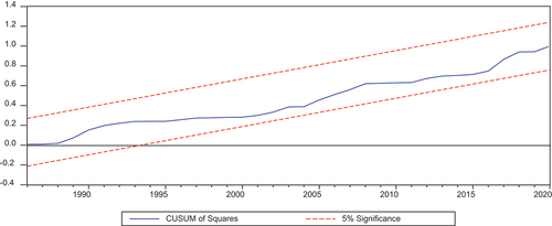
From table 10 above, the residual diagnostic tests show that the study residuals are not heteroscedastic, while the Jarque-Bera shows that residuals are normally distributed. Further, the our model choice fits the data well. Finally we also find that there is no serial correlation. The model stability test for both the short and long is based on both the cumulative sums of recursive residuals (CUSUM) and cumulative sums of recursive residuals squared (CUSUMQ). From Figures 2 and 3 below, since the curve (i.e. blue line) lies within the 5% confidence interval (i.e. lower and upper critical lines), it is indicative that the model fitted in this study is stable, and therefore there is no risk of any structural break in the models fitted in both short and long-run. Diagnostic tests (i.e. Stability test) are a recommendation from (Pesaran et al., 2001) seminal work on the Bounds approach to cointegration. According to Pesaran, diagnostic tests help to avoid obtaining spurious results (See Figure 4).

Table 10. VECM model diagnostic test

Diagnostic test	Test for	p-value	Conclusion
VEC Heteroskedasticity Tests	Heteroscedasticity	63.504 (.066)	Not Heteroscedastic
Jarque-Bera	Normality	6.03 (.214)	Residuals are normal
Goodness of Fit	R-Square Test	.6859	There is a good fit
Autocorrelation LM test	serial correlation	122.27 (.83)	No serial correlation

Source: Authors’ computations from Eviews 10.

Figure 3. CUSUM measure of model stability.

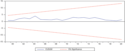
Figure 4. Graph of the Cumulative Sum of Squares (Cusumq).

4.7. Causality tests

After estimating the VECM model, it is worthwhile to perform causality tests (Engle & Granger, 1987). Below, we discuss the causality test results (see Table A4). Considering the results above, since THR is significant at a 1% level of significance, we reject the null of no causality between the service sector total value added and THR services in the short run and conclude that there is a short-run causal relationship from THR to services. Similarly, STC, FC, LS, MU, and MA have a short-run causal relationship with the services sector total value added. While the fisheries, and construction sub-sectors do not have a short-run causal relationship with the services sector. In Uganda, communication services (i.e. print media, TVs, Radio, and Telecom) specifically, the telecommunication services have been the fastest growing sub-sector overall in the services sector. On the other hand, FC, fisheries, LS, MA, and MU have a short-run causal relationship with the THR services, while the performance of the services sector has a strong causal relationship with the STC and MU. Overall, the variables included in this model have a causal relationship with total services value added (SER), THR, and STC, this indicates the role that the services sector plays in Uganda’s economy. This result is supported by findings in studies such as (Ggoobi et al., 2017; Shinyekwa et al., 2016), who analyzed Ugada’s industrial sector performance over the years.

Results from the pairwise Granger causality test are reported in Table A4, we observe that THR Granger causes Services but Services does not Granger cause THR hence a unidirectional causality. On the other hand, MA Granger causes Services while services do not Granger cause MA which is a unidirectional causality. An independent causality is found between construction and services, while a unidirectional causality is reported between STC and MA, and STC and construction, an independent relationship between THR and construction, lastly, the only bidirectional relationship Is that between THR and fisheries sector.

4.8. Forecast Error Variance Decomposition (FEVD)

Variance Decomposition provides the percentage of unexpected variance in each variable that is produced by shocks from other variables. In other words, it indicates the relative impact that a variable has on another (Lütkepohl, 2005). From Table A5, results under the services sector indicate that 45.85% of the forecast error variance is explained by the agriculture sector in the short run, and the contribution of the agricultural sector towards the services sector increases into the future reaching 50.52% in the fifth year, implying a strong endogenous influence on the services sector. The influence of the industrial sector on the services sector decreases in the future. Finally, 30.28% of the forecast error variance is explained by changes in the services sector itself, but as we move further into the future, the sector exhibits a moderately strong endogenous influence on itself. The influence of the services sector increases in the short to long run. This implies that the services sector exhibits a strong endogenous influence on the industrial sector. In conclusion, FEVD indicates that a substantial amount of variation in each sector is explained by its shocks rather than shocks from other sectors, therefore, both the independent causality between service and industry and the unidirectional causality between agriculture and services and industry are reconfirmed (Table A6).

5. Discussion of results

The overall objective of this study was to examine the production and consumption inter-sectoral linkages in Uganda’s economy. Specifically, the emphasis was put on analyzing multiplier effects based on the Social Accounting Matrix (SAM) for Uganda (i.e. SAM 2009/10 and SAM 2016/16). The results of the SAM model were reconfirmed through a series of robust checks based on the VECM model and its related diagnostic checks. We estimate the VECM because it explains the relationship between endogenous and exogenous variables’ dynamic behavior and that of the endogenous variables. Further, this framework uses granger causality analysis and impulse response functions (IRF) to describe how a variable or collection of variables affects others. Which clearly suits our current study.

Available reports from World Bank, UBOS, BOU, and MFPED all point to the fact that Uganda’s economy is driven largely by the rapidly growing services sector. However, there is a paucity of empirical evidence that quantify the impact of the services sector multiplier effects on other sectors (i.e. in terms of direct, indirect, forward, and backward linkages), to ascertain if the observed services sector growth is trickling down to other sectors. The reason for this analysis is that although Uganda’s economy is still largely agrarian in terms of employment, over 50% of the country’s growth is derived from the services sector. Therefore, understating inter-sectoral linkages dynamics between these sectors is important for policy. Based on the multiplier model results in Table 11, the services sector had the highest output multiplier effect at 3.13 units from demand. At the aggregate level, the service sector is the top output-generating sector followed by agriculture. This is indicative of the strong integration of the services sector into other sectors. The services sector also emerges strong in terms of GDP multipliers, recorded at 1.87 units followed by agriculture (1.51) and the industrial sectors (0.82) units respectively in case of a demand shock.

Table 11. Sectoral production linkages in Uganda

	SAM 2009/10			SAM 2016/17
	Agriculture	Industrial	Services	Agriculture	Industrial	Services
Agriculture	1.29	0.37	0.52	1.17	0.34	0.30
Industrial	0.44	0.87	0.71	0.38	0.94	0.39
Services	0.54	0.37	1.90	0.72	0.59	2.02
Total sectoral income	2.27	1.61	3.13	2.27	1.87	2.71
Forward linkages	0.89	1.15	0.91	0.63	0.76	1.32
Backward linkages	0.98	0.74	1.23	1.10	0.93	0.68

Source: Authors’ Computation-SAM-based Multiplier model output.

On the other hand, in 2016/17, a one-unit income injection across the sectors increased the agricultural sector GDP by 1.56 units compared to 1.39 and 1.06 units for the services and industrial sectors respectively. Again, the services sector produced the highest household and consumption multiplier effects in 2009/10 and 2016/17 at 1.44 and 1.15 units and 2.89 and 1.82 units. The strong performance of the services sector is indicative of the recently growing strong role that the services sector plays in Uganda’s economy.

Although the services sector had the highest sectoral income reported at (3.13) units in 2009/10 and (2.71) units in 2016/17 (see results in Table 3). The industrial sector had the strongest forward linkages (1.15) compared to services (0.91) and agriculture (0.89). However, the services sector had the strongest backward linkages (1.23) these linkages were stronger with the industrial sector (0.71) vis-à-vis agriculture (0.53). In 2016/17, the services sector had the strongest forward linkages (1.32) and these linkages were stronger with agriculture (0.72) compared to the industrial sector (0.59). The results from the VECM model indicate that in the long run, the industrial sector (lnIN) hurts the agricultural sector while the services sector has a positive impact on the agricultural sector ceteris paribus and the coefficients are statistically significant at a 1% level of significance. Again considering the Johansen normalized vectors, the null hypothesis of cointegration is rejected against the alternative cointegration relationship in the model. These results are in line with Singh (2015) who found strong and weak long and short-run linkages respectively among sectors in India. To him, causality was a short-run rather than a long-run phenomenon.

Disaggregating the sectoral effect, a one-unit income injection in the livestock sector (LS) increases the agricultural gross output by 2.93 units compared to 2.59 if injections were inserted into the food crop and cash crop sub-sectors. Construction (3.22) and mining (3.17) were the leading gross output-generating industrial sub-sectors, while SCT (7.91) and FIN (4.09) were the highest gross output-generating sectors in 2016/17, this is indicative of the higher level of integration with other sectors in the economy. Conversely, SCT and FIN generated the highest value-added among the services sub-sectors, signifying higher integration and inter-sectoral linkages in the domestic factor markets. In terms of income multipliers, utilities (ELGW), FIN, and HE in the services sector generated the highest income for households. Similarly, The SCT, FIN, and HE generated the highest consumption multipliers for the services sector. In 2009/10, SCT recorded the strongest forward linkages (1.68), while (HE) had the strongest backward linkages (0.75). The SCT’s forward linkages were strongest with financial services (0.41) and trade hotel and restaurant THR (0.19), while its backward linkages were strongest with the financial services (0.24), and manufacturing services (0.20). On the other hand, in 2016/17 the services sub-sectors showed that forward and backward linkages were strongest for SCT and FIN at 6.33 and 1.43 for the forward linkages and 3.90 and 3.05 for backward linkages, respectively.

In this study, we further tested the possibilities of constrained sectoral supply, given that Uganda’s economy is still largely agrarian, we test the impact of constrained supply in the agricultural sector on other sectors. Results from Table 3 indicate that a million shilling increase in agricultural exports lead to 1.29, 0.44, and 0.54 million shillings in 2009/10 and 1.17, 0.38, and 0.72 million shillings increase in 2016/17 for the agricultural, industrial and the services sectors respectively. The results in Table 3 also point to Uganda’s export dependence since the increase in agricultural export leads to excess demand in the industrial sector. In the unconstrained scenario, a similar increase in the industrial export demand stimulates services sector output by 1.90 million compared to the demand of 1.92 million shillings similar impacts have been reported by (Breisinger et al., 2010) in Ghana. The decline in the agricultural value added as the industrial sector expands can be due to the population effect, Uganda’s youth population is less attracted to the agricultural sector in favor of white-collar jobs in the industrial and services sectors (Byiers et al., 2015; Ggoobi et al., 2017; Shinyekwa et al., 2016).

The Pairwise Granger Causality tests results reveal three relationships, i.e. a unidirectional causality from the agricultural sector to the industrial and the services sectors, and an independent relationship from the industrial to the services sector. This implies that shocks in the agricultural sector will spill over to both the industrial and the services sectors but the reverse may not be true always. These causality effects are just short-run phenomena. Meanwhile, the negative impact of the industrial sector on the agricultural sector in the short run could be due to the increased competition for the factors of production. Conversely, the forward linkage between the agricultural and the industrial sectors occurs when industries utilize agricultural output in their production process for example the agro-processing firms.

Finally, the strong growth in the services sector can explain the positive impact of the services sector on the agricultural sectors. Furthermore, due to the competition for financial resources in the services sector, there can be selective loan approval to different sectors by financial institutions, particularly the low-risk sectors with high returns will be funded. However, in the long run, growth in the industrial sector can stimulate demand for agricultural products leading to positive linkages. In conclusion, both agricultural and industrial sectors have benefited from the rapidly growing services sector. For example, improvements in services such as storage, transport, and communication (STC), and insurance and banking (IB) can explain the existence of positive backward linkage of the services sector to the agricultural and industrial sectors. Therefore, sectoral policies should be based on how sectors interrelate in both the short and long-run scenarios, and also sectoral constraints should be embedded in sectoral forecasting and planning.

6. Conclusions and policy recommendations

The overall objective of this study was to examine inter-sectoral linkages in Uganda’s economy. The SAM-multiplier model examines the impact of a demand shock. First at the aggregated sector level, and second at the sub-sector level. Third, given that sectoral productivity is susceptible to supply constraints, especially in the agricultural sector, two scenarios are tested namely elastic and inelastic agricultural sector supply scenarios. At the aggregate level, the services sector had the highest sectoral income reported at (3.13) units in 2009/10 and (2.71) units in 2016/17. In 2009/10, the industrial sector had the strongest forward linkages (1.15) while the services sector had the strongest backward linkages (1.23). The service sector’s linkages were stronger with the industrial sector (0.71) vis-à-vis agriculture (0.53). In 2016/17, the services sector had the strongest forward linkages (1.32) and these linkages were strongest with agriculture (0.72) units. At a disaggregated level, the SCT recorded the strongest forward linkages (1.68), while (HE) had the strongest backward linkages (0.75) in 2009/10. The SCT’s forward linkages were strongest with financial services (0.41) while its backward linkages were strongest with the financial services (0.24). In 2016/17, SCT had the strongest forward and backward linkages at 6.33 and 3.90 units respectively.

To implement robust checks for the SAM Multiplier, the VECM time series model was estimated following four stages. First, time series were tested for stationarity, the goal is to work with non-stationary series. Second, a cointegration test was performed based on Johansen’s (1991) Cointegration procedure. The third stage involved estimating the VECM. Three unit root tests were estimated namely ADF, PP, and KPSS tests, which all indicated evidence for stationarity after fast difference, lag selection was based on the Akaike information criterion (AIC). Overall, we reject the null hypothesis that there is no cointegration equation in the model at a 5% level of significance, implying that the series are cointegrated and exhibit a long-run relationship and can thus be combined linearly in analysis (Johansen, 1991). The key finding in this study is that inter-sectoral linkages can take place in both the short and the long run. Secondly, the sectors considered in this study exhibit both positive and negative linkages in both the short and the long-run time. Therefore, policymakers should consider the aspect of time in sectoral policy formulation.

Although the services sector has overtaken the agricultural sector as the driver of growth, the results from the VEC model suggest that the agricultural sector still plays a major role in determining the overall economic growth in Uganda through its linkages to other sectors. The key policy message is that government should equally redistribute its policy priorities from focusing mainly on industrialization towards stimulating domestic demand in agricultural sector, especially in rural areas where subsistence agriculture is still dominant. Incidentally, government needs to review and refocus its already existing sectoral growth strategies and programs before starting new ones. We find evidence that storage, communication, and transport (SCT) has strong linkages in the services sector. Thus, government must improve transport and communication networks. The cost of ICT products and services should be fully regulated by the government to ensure that online business can thrive across all sectors.

Government should rebalance its sectoral growth acceleration agenda from over-emphasizing agriculture (i.e. the inward-looking) type of policies to focusing on other sectors in the growth mix (i.e. outward-looking) type of policies. On the other hand, the persistent decline in the agricultural sector’s contribution to overall growth over the years has led to a decline in the demand-generating capacity of the agricultural sector to other sectors. Incidentally, there is a need to review agricultural sector-related incentives, such as tax holidays and subsidies for those willing to engage in commercial agriculture. There should be equity and efficiency in incentivizing the sector actors.

Results indicate that the contribution of the industrial sector has hovered around 25% for the last 30 years, therefore there is a need for the government to review and reorient both its industrial policy and industrialization strategy. Government needs to develop a competitive, internationally focused, and highly productive industrial sector to increase industrial exports, create employment to absorb surplus labor from the agricultural sector, and stimulate productivity spillovers.

Government should strengthen the linkages between the agricultural and the industrial sectors through investment in agriculture so that the industrial sector gains from the agricultural sectors’ comparative advantage to engage in the agro-processing of crops such as coffee, cotton, and other food crops. In addition, the government should diversify its exports of goods and services and also spread its trading partners to avoid being vulnerable to external shocks during economic downturns. Further, the government should take advantage of the excess capacity in the agricultural sector through increased targeted sub-sector investment to enhance inter-sectoral linkages.

Authors’ contributions

MJ is the leading author of the manuscript; he initiated the research idea, undertook a literature review, developed the theoretical framework, and collected and analyzed the data from different sources. HE and MI are co-authors of this manuscript. They approved the research idea and supervised the entire manuscript preparation from start to finish. Further, they provided quality assurance, and guidance, and approved the final manuscript.

Authors’ information

MJ is a Ph.D. student at the School of Economics at Makerere University and an assistant lecturer at the School of Statistics and Planning at the same university. MJ is a young professional in research with a strong bias in Monetary, Public sector economics, Labour Economics, and Impact Evaluation. He is the 2021 Center for Global Effective Action Fellow at the University of California at Berkeley. HE is a Professor of Economics and the Principle of the College of Business and Management Sciences. MI is the coordinator of the graduate programs at the school of economics at Makerere University and a senior lecturer.

Availability of data and materials

This study used two sources of data, first data was sources from two Uganda Social Accounting Matrices (SAM) for the years 2009/10 and 2016/17. The data on the SAMs is available at the Ministry of Finance Planning and Economic Development (MFPED) and the Uganda Bureau of Statistics (UBOS). The SAMs data was supplemented by a long time series data spanning the period 1980–2020, this data is available at the World Bank development indicators website see; https://databank.worldbank.org/source/world-development-indicators.

Acknowledgments

We extend our sincere gratitude to the academic staff of the school of Economics of Makerere University who provided helpful insights and comments to improve this study. We thank the Dean of the school of economics and the head of the department of Planning and Applied Economics. We also thank all fellow students of the Ph.D. in economics at Makerere University class of 2018/19 for the support and valuable comments that improved this work.

Disclosure statement

No potential conflict of interest was reported by the authors.

Additional information

Funding

This study did not receive any funding.

Notes on contributors

Mukoki James

Mukoki James is a Ph.D. candidate (Economics) at Makerere University in Uganda. He holds a Master of Arts degree in Economics (MA) from the University of Dar es Salaam, Tanzania. He poses over ten years of research experience in developing countries. His research interest lies in the areas of macroeconomics, development and applied economics, Labor economics, and Public Health. He is a 2021-2022 CEGA fellow, where he gained a lot of experience in the design of field experiments and Randomized Control trials (RCTs).

Hisali Eria

Hisali Eria is a Professor of Economics and Principle of the College of Business and Management Sciences (CoBAMS) at Makerere University. He is a seasoned academic whose research has made a significant contribution to the scholarly body of knowledge both in Africa and internationally.

Mukisa Ibrahim

Mukisa Ibrahim (Ph.D.) is a seasoned academician and researcher, he is the Coordinator of graduate programs at the School of Economics at Makerere University. Our research related to the persistent underdevelopment and unemployment that ravage most of the developing world.

Appendices

Table A1. SAM 2016/17 inter-sectoral linkages and exogenous demand shock

1 unit injection	Agriculture				Industry			Services
Sectors	Crop	Livest	Forest	Fish	Min	Man	Cons	ELGW	SCT	THR	FIN	HE
Crop	1.06	0.24	0.24	0.23	0.23	0.22	0.24	0.25	0.35	0.30	0.27	0.29
Livestock	.05	1.02	0.06	0.06	0.06	0.07	0.07	0.06	0.09	0.07	0.07	0.07
Forestry	.05	0.06	0.88	0.06	0.12	0.05	0.11	0.06	0.13	0.06	0.07	0.09
Fishing	.03	0.04	0.04	0.85	0.03	0.03	0.04	0.04	0.05	0.04	0.04	0.04
Mining	.01	0.02	0.01	0.01	0.85	0.03	0.08	0.01	0.04	0.02	0.02	0.02
Manufacture	.35	0.46	0.38	0.37	0.46	0.75	0.54	0.40	1.09	0.47	0.52	0.49
ELGW	.06	0.07	0.06	0.06	0.07	0.05	0.06	1.07	0.11	0.08	0.09	0.08
TCT	.39	0.42	0.43	0.43	0.60	0.31	0.44	0.48	4.01	0.59	0.95	0.60
HR	.08	0.08	0.09	0.09	0.09	0.06	0.08	0.09	0.14	1.04	0.11	0.11
FIN	.06	0.07	0.07	0.07	0.09	0.05	0.07	0.08	0.41	0.10	1.04	0.10
HE	.12	0.12	0.13	0.13	0.11	0.08	0.12	0.13	0.10	0.12	0.13	1.13
Total income	2.59	2.93	2.74	2.71	3.17	1.95	3.22	3.08	7.91	3.30	4.09	3.47
Forward	3.10	0.79	0.93	0.44	0.29	5.96	0.01	0.88	6.33	1.12	1.43	1.41
Backward	1.53	1.91	1.86	1.86	2.32	1.20	2.23	2.00	3.90	2.26	3.05	2.33
Direct effects	1.06	1.02	0.88	0.85	0.85	0.75	0.99	1.07	4.01	1.04	1.04	1.13
Indirect effects	3.10	0.79	0.93	0.44	0.29	5.96	0.00	0.88	6.33	1.12	1.33	1.41

Source: Authors Computation from SAM-based Multiplier model; Notes: Min is mining, Man: manufacturing sector, Elgw is electricity, Tct is Trade communication and transport, Hr is hotel and restaurant, Fin is financial, insurance and business services, He is education and health services.

Table A2. Correlation matrix

Variables	CC	FC	FT	LS	FH	Manu	MU	Const	THR	STC	OS
Cash Crop	1.00
Food crop	0.26	1.00
Forestry	0.45	0.60	1.00
Livestock	0.25	0.74	0.31	1.00
Fisheries	0.58	0.40	0.56	0.65	1.00
Manu	0.06*	0.71*	0.78*	0.48*	0.57*	1.00
MU	0.79*	0.59*	0.69*	0.49*	0.19*	0.22*	1.00
Const	0.73*	0.43*	0.73*	0.33*	0.53*	0.80*	0.28*	1.00
THR	0.61*	0.16*	0.76*	0.76*	0.61*	0.56*	0.71*	0.14*	1.00
STC	0.71*	0.89*	0.89*	0.89*	0.69*	0.71*	0.67*	0.46*	0.75*	1.00
OS	0.44*	0.49*	0.49*	0.49*	0.49*	0.49*	0.49*	0.67*	0.79*	0.70*	1.00

Source: Authors compilation.

Table A3. Johansen/Unrestricted cointegration rank test

Hypothesized No. of CE(s)	Test (Trace)			Max Eigenvalue
	Trace Statistic	0.05 Critical Value	Prob.**	Max-Eigen Statistic	0.05 Critical Value	Prob.**
None	391.88	285.14	0.00	97.06	70.54	0.00
At most 1	294.82	239.24	0.00	77.15	64.50	0.00
At most 2	217.67	197.37	0.00	52.29	58.43	0.18
At most 3	165.39	159.53	0.02	47.15	52.36	0.16
At most 4	118.24	125.62	0.13	37.27	46.23	0.33
At most 5	80.97	95.75	0.33	28.16	40.08	0.55
At most 6	52.81	69.82	0.51	20.55	33.88	0.72
At most 7	32.26	47.86	0.60	14.54	27.58	0.78
At most 8	17.72	29.80	0.59	11.93	21.13	0.55
At most 9	5.79	15.49	0.72	5.23	14.26	0.71
At most 10	0.56	3.84	0.45	0.56	3.84	0.45

Source: Authors’ computations, Notes: Trace test indicates 1 Cointegration equation(s) at the 0.05 level, *, Max-eigenvalue test indicates 1 Cointegration equation(s) at the 0.05 level, * denotes rejection of the hypothesis at the 0.05 level, while **MacKinnon-Haug-Michelis-(1999), p-values, the lag selection is based on Hannan-Quinn criterion and Schwarz information criterion (AIC).

Table A4. VEC granger causality/block exogeneity wald tests

Sectors	Service			Agriculture			Industrial sector
Variables	SER	THR	STC	FC	FISH	LS	MA	MU	CONST
SER	-	3.46	5.48***	0.59	2.75	0.50	0.80	0.43	1.26
THR	14.44*	-	0.92	2.09	1.54	0.26	7.47	0.17	1.51
STC	5.76***	3.31	-	0.24	1.11	1.19	0.49	0.40	0.13
FC	6.69**	19.58*	1.56	-	4.79***	0.28	3.23	0.90	10.43**
FISH	2.64	21.84*	0.64	3.43	-	1.79	5.20***	2.69	0.82
LS	12.07**	8.14*	2.02	1.02	0.48	-	0.67	0.75	2.67
MA	9.48*	7.49*	4.12	0.12	0.64	1.60	-	0.25	0.24
MU	1.55*	4.62***	11.25*	0.63	0.38	0.52	2.22	-	4.84***
CONST	1.78	0.49	3.67	0.17	4.91***	3.23	0.55	1.32	-
All	35.73*	46.76*	28.76**	10.57	17.48	12.19	21.36	7.28	18.52

Notes: “-” indicates a dependent variable, p values of coefficients: ***p < 0.01, **p < 0.05, and *p < 0.1; Source: Authors computation.

Table A5. Forecast Error Variance Decomposition (FEVD)

year	Var Decomposition of LNAG				Var Decomposition of LNIN				Var Decomposition of LNSS
	S.E.	lnAG	lnIN	lnSS	S.E.	lnAG	lnIN	lnSS	S.E.	lnAG	lnIN	lnSS
1	0.221	100.00	0.00	0.00	0.226	50.29	49.71	0.00	0.199	45.85	23.88	30.28
2	0.358	99.86	0.13	0.01	0.312	51.79	47.83	0.38	0.274	56.99	20.76	22.25
3	0.459	99.49	0.15	0.36	0.375	47.11	46.53	6.36	0.344	55.44	19.21	25.35
4	0.538	98.75	0.12	1.12	0.426	41.68	44.23	14.09	0.398	53.41	17.79	28.79
5	0.602	97.78	0.09	2.12	0.474	36.19	41.38	22.43	0.448	50.52	16.63	32.85

Source: Authors’ computation based on VECM output from Eviews10, Notes: S.E. denotes the standard error. Cholesky ordering: [lnAG, lnIN, lnSS].

Table A6. VECM-Short run output

Variables	D(LN_SER)	D(LN_THR)	D(LN_STC)	D(LN_FC)	D(LN_FISH)	D(LN_FT)	D(LN_LS)	D(LN_CONST)	D(LN_MA)	D(LN_MU)
D(LN_SER(−1))	−0.274 -(0.166)	−0.112 -(0.080)	−0.234 -(0.076)	−0.061 -(0.257)	−0.165 -(0.101)	0.246 -(0.147)	−0.151 -(0.196)	−0.102 -(0.179)	−0.131 -(0.196)	−0.104 -(0.144)
D(LN_SER(−2))	−0.346 -(0.152)	−0.022 -(0.073)	0.096 -(0.070)	−0.231 -(0.236)	−0.315 -(0.093)	0.112 -(0.135)	0.029 -(0.179)	−0.051 -(0.164)	−0.199 -(0.180)	−0.074 -(0.132)
D(LN_THR(−1))	−0.748 -(0.425)	0.321 -(0.204)	0.063 -(0.195)	−0.147 -(0.658)	0.484 -(0.259)	−0.137 -(0.375)	0.019 -(0.500)	−0.436 -(0.456)	0.949 -(0.501)	−0.226 -(0.368)
D(LN_THR(−2))	1.191 -(0.400)	0.018 -(0.192)	−0.123 -(0.183)	−1.063 -(0.619)	0.162 -(0.244)	−0.035 -(0.353)	0.054 -(0.471)	−0.156 -(0.430)	−0.375 -(0.472)	0.131 -(0.347)
D(LN_STC(−1))	0.128 -(0.372)	−0.178 -(0.179)	−0.060 -(0.171)	0.087 -(0.577)	−0.263 -(0.227)	0.053 -(0.329)	−0.194 -(0.439)	−0.004 -(0.400)	−0.394 -(0.440)	−0.067 -(0.323)
D(LN_STC(−2))	−0.512 -(0.333)	0.183 -(0.160)	0.078 -(0.153)	−0.018 -(0.516)	0.183 -(0.203)	−0.055 -(0.294)	−0.312 -(0.392)	−0.034 -(0.358)	0.259 -(0.393)	−0.167 -(0.289)
D(LN_FC(−1))	0.585 -(0.287)	0.185 -(0.138)	0.109 -(0.132)	−0.831 -(0.445)	0.756 -(0.176)	−0.167 -(0.254)	0.585 -(0.339)	0.011 -(0.309)	0.230 -(0.339)	−0.042 -(0.249)
D(LN_FC(−2))	0.142 -(0.173)	0.162 -(0.083)	0.056 -(0.079)	−0.299 -(0.268)	0.437 -(0.106)	−0.197 -(0.153)	0.227 -(0.204)	0.284 -(0.186)	0.075 -(0.204)	−0.043 -(0.150)
D(LN_FISH(−1))	−0.177 -(0.232)	0.214 -(0.112)	0.063 -(0.107)	0.564 -(0.360)	−0.753 -(0.142)	−0.006 -(0.205)	0.526 -(0.274)	0.214 -(0.250)	0.117 -(0.274)	0.005 -(0.202)
D(LN_FISH(−2))	0.074 -(0.237)	0.098 -(0.114)	0.079 -(0.109)	0.155 -(0.367)	−0.382 -(0.145)	−0.141 -(0.209)	0.082 -(0.279)	0.191 -(0.255)	−0.441 -(0.280)	0.284 -(0.205)
D(LN_FT(−1))	−0.696 -(0.331)	−0.171 -(0.159)	−0.092 -(0.152)	0.655 -(0.513)	−0.195 -(0.202)	−0.456 -(0.292)	−0.542 -(0.390)	0.334 -(0.356)	0.159 -(0.391)	0.044 -(0.287)
D(LN_FT(−2))	−0.018 -(0.274)	−0.073 -(0.132)	−0.022 -(0.126)	0.087 -(0.425)	−0.122 -(0.168)	−0.083 -(0.242)	−0.307 -(0.323)	0.011 -(0.295)	0.098 -(0.324)	0.196 -(0.238
D(LN_LS(−1))	0.230 -(0.191)	0.106 -(0.092)	0.108 -(0.088)	−0.028 -(0.296)	0.423 -(0.117)	0.029 -(0.169)	−0.603 -(0.225)	−0.261 -(0.205)	0.083 -(0.225)	0.026 -(0.166)
D(LN_LS(−2))	0.410 -(0.166)	0.103 -(0.080)	0.036 -(0.076)	−0.048 -(0.257)	0.282 -(0.101)	0.100 -(0.146)	−0.410 -(0.195)	0.000 -(0.178)	−0.042 -(0.196)	0.064 -(0.144)
D(LN_CONST(−1))	0.209 -(0.167)	0.025 -(0.080)	0.065 -(0.077)	0.009 -(0.259)	−0.185 -(0.102)	0.255 -(0.148)	0.022 -(0.197)	−0.640 -(0.180)	−0.084 -(0.198)	0.130 -(0.145)
D(LN_MA(−1))	0.303 -(0.179)	−0.096 -(0.086)	−0.012 -(0.082)	−0.011 -(0.277)	−0.029 -(0.109)	0.156 -(0.158)	−0.018-(0.211)	0.053 -(0.192)	−0.305 -(0.211)	−0.065 -(0.155)
D(LN_MU(−1))	0.360 -(0.263)	0.162 -(0.126)	0.398 -(0.121)	−0.218 -(0.407)	0.090 -(0.161)	−0.159 -(0.232)	−0.019 -(0.310)	0.019 -(0.283)	−0.309 -(0.311)	−0.258 -(0.228)
C	0.138	0.074	−0.053	0.151	−0.004	0.075	0.087	0.065	−0.020	0.112

References

- Amano, M. A. (1980). A neoclassical model of the dual economy with capital accumulation in agriculture. The Review of Economic Studies, 47(5), 933–36. https://www.jstor.org/stable/2296923
- Barrett, C. B., Carter, M. R., & Timmer, C. P. (2010). Acentury-long perspective on agricultural development. American Journal of Agricultural Economics, 92(2), 447–468. https://doi.org/10.1093/ajae/aaq005
- Baumol, W. J. (1967). Macroeconomics of unbalanced growth: The anatomy of urban crisis. The American Economic Review, 57(3), 415–426.
- Breisinger, C., Marcelle, T., & Thurlow, J. (2010). Social accounting matrices and multiplier analysis: An introduction with exercises. International Food Policy Research Institute (IFPRI).
- Bwire, T., Asiimwe, W., Tinyinondi, Grace, A., Kisakye, P., & Ayume, D. (2016). Private and public investments and economic growth in Uganda: A multiplier model analysis (Issue 01). Bank of Uganda Working Paper No. 01/2016.
- Byiers, B., Takeuchi, L. R., Rosengren, A., Muhwezi, M., Turyareeba, D., Abaliwano, J., Wabukala, B., & Ggoobi, R. (2015, March). Work in progress productive employment and transformation in Uganda. Overseas Development Institute (ODI).
- Chenery, H. B. (1982). Industrialization and growth: The experience of large countries. World Bank Staff Working Paper, 539(539).
- Clement, C. (2015). The formal-informal economy dualism in a retrospective of economic thought since the 1940s. Schriftenreihe Des Promotionsschwerpunkts Globalisierung Und Beschäftigung, 43. https://nbn-resolving.de/urn:nbn:de:bsz:100-opus-10572This
- Dabús, C., & Delbianco, F. (2021). Economic development and structural change: The role of services. Journal of Economic Development, 46(3), 65–84.
- Defourny, J., & Thorbecke, E. (1984). Structural path analysis and multiplier decomposition within a social accounting matrix framework. The Economic Journal, 94(373), 111–136. https://doi.org/10.2307/2232220
- Dickey, D., & Fuller, W. (1981). Likelihood ratio statistics for autoregressive time series with a unit root. Econometrica, 49(4), 1057–1072. https://doi.org/10.2307/1912517
- Engle, R. F., & Granger, C. W. J. (1987). Co-integration and error correction: Representation, estimation, and testing. Applied Econometrics, 39(3), 107–135. https://doi.org/10.2307/1913236
- Feder, G. (1982). On export and economic growth. Journal of Development Economics, 12(1–2), 59–73. https://doi.org/10.1016/0304-3878(83)90031-7
- Gemmell, N. (1982). Economic development and structural change: The role of the service sector. The Journal of Development Studies, 19(1), 37–66. https://doi.org/10.1080/00220388208421849
- Gemmell, N., Lloyd, T. A., & Mathew, M. (2000). Agricultural growth and inter-sectoral linkages in a developing economy. Journal of Agricultural Economics, 51(3), 353–370. https://doi.org/10.1111/j.1477-9552.2000.tb01236.x
- Gemmell, N., Lloyd, T., & Mathew, M. (1998). Dynamic sectoral linkages and structural change in a developing economy. 98(3), 1–25. http://www.nottingham.ac.uk/credit/documents/papers/98-03.pdf
- Ggoobi, R., Wabukala, B. M., & Joseph, N. (2017). Economic development and industrial policy in Ugnada. In Applied Geography. https://doi.org/10.1016/0143-6228(95)90025-x
- Gollin, B. D., Parente, S., & Rogerson, R. (2002). The role of agriculture in development. American Economic Review, 92(2), 160–164. https://doi.org/10.1257/000282802320189177
- Haggblade, S., Hazell, P., & Reardon, T. (2010). The rural non-farm economy: prospects for growth and poverty reduction. World Development, 38(10), 1429–1441. https://doi.org/10.1016/j.worlddev.2009.06.008
- Jami, H. M. (2006). A SAM-based multiplier model to track growth-poverty-inequality nexus in Bangladesh. Munich Personal RePec Archive, 13517. https://mpra.ub.uni-muenchen.de/13517/
- Johansen, S. (1989, January). Estimation and hypothesis testing of cointegration vectors in gaussian vector autoregressive models. Econometrica, 3(2), 216–249.
- Johansen, S. (1991). Estimation and hypothesis testing of cointegration vectors in gaussian vector autoregressive models. Econometrica, 59(6), 1551–1580. https://doi.org/10.2307/2938278
- Jorgenson, D. W. (1961). The structure of multi-sector dynamic models. International Economic Review, 2(3), 276–293. https://doi.org/10.2307/2525432
- Kaur, G., Bordoloi, S., & Rajesh, R. (2009). An empirical investigation on the inter-sectoral linkages in India an empirical investigation of the inter-sectoral linkages in India. Munich Personal RePEc Archive, 1(40419), 29–72. https://mpra.ub.uni-muenchen.de/40419/
- Kwiatkowski, D., Phillips, P. C., & Schmidt, P. (1991). Testing the null hypothesis of stationarity againts the alternative of a unit root: How sure are we that economic time series have a unit root?
- Lewis, W. (1954). Economic development with unlimited supplies of labour. The Manchester School, 30(2), 139–191. https://doi.org/10.1111/j.1813-6982.1962.tb02428.x
- Llop Llop, M. (2005). Comparing multipliers in the social accounting matrix framework. Department d’Economia, Universitat Rovira i Virgili.
- Lütkepohl, H. (2005). New introduction to multiple time series analysis. New Introduction to Multiple Time Series Analysis. https://doi.org/10.1007/978-3-540-27752-1
- Mainar-Causapé, A. J., Emanuele, F., & Scott, M. (2018). Social accounting matrices: Basic aspects and main steps for estimation. https://doi.org/10.2760/010600
- Matovu, J. M. (2000). Composition of government expenditure, human capital accumulation, and welfare. International Monetary Fund.
- Mlambo, C., Mukarumbwa, P., Megbowon, E., & Aye, G. (2019). An investigation of the contribution of processed and unprocessed agricultural exports to economic growth in South Africa. Cogent Economics & Finance, 7(1), 1694234. https://doi.org/10.1080/23322039.2019.1694234
- Muwonge, A., Obwana, M., & Nambwaayo, V. (2007). Enhancing contributions of the informal sector to National development: The case of Uganda. Economic Policy Research Center (EPRC). https://eprcug.org/publications/occasional-papers/
- Newey, W. K., & West, K. D. (1987). A simple, positive semi-definite, heteroskedasticity and autocorrelation consistent covariance matrix. The Economertric Society, 55(3), 703–708. https://doi.org/10.2307/1913610
- Nguyen, C. H., Chuong, H. N., & Trung, T. (2022). Linkages and development of local industrial space: Research in the key economic region of Southern Vietnam. Cogent Economics & Finance, 10(1). https://doi.org/10.1080/23322039.2022.2109273
- Nnyanzi, J. B., Oryema, J. B., & Kilimani, N. (2022). Real exchange rate undervaluation, regional integration and services sector performance: Evidence from the East African Community. Journal of Economic Structures, 11(1), 3. https://doi.org/10.1186/s40008-022-00279-3
- Ogbonna, O. E., Mobosi, I. A., Ugwuoke, O. W., & McMillan, D. (2020). Economic growth in an oil-dominant economy of Nigeria: The role of financial system development. Cogent Economics & Finance, 8(1), 1810390. https://doi.org/10.1080/23322039.2020.1810390
- Onakoya, B. A. (2013). Agriculture and intersectoral linkages and their contribution to Nigerian economic growth. Economics, 2(5), 38–54. https://doi.org/10.11648/j.eco.20130205.11
- Pesaran, M. H., Shin, Y., & Smith, R. J. (2001). Bounds testing approaches to the analysis of level relationships. Journal of Applied Econometrics, 16(3), 289–326. https://doi.org/10.1002/jae.616
- Phillips, P. C. B., & Perron, P. (1988). Testing for a unit root in time series regression. Biometrika, 75(2), 335–346. https://doi.org/10.1093/biomet/75.2.335
- Phoofolo, M. L. (2018, March). Analysis of the economic impact of a disaggregated agricultural sector in South Africa: A Social Accounting Matrix (SAM) multiplier approach. https://scholar.sun.ac.za
- Punt, C. (2013 March). Modelling multi-product industries in Computable General Equilibrium (CGE) models. SUNScholar. https://scholar.sun.ac.za/handle/10019.1/79959
- Pyatt, G., & Round, J. I. (1985). Social Accounting Matrices a basis for Planning. The World Bank.
- Randriamamonjy, J., & Thurlow, J. (2017). 2013 Social accounting matrix for Uganda: A nexus project SAM. International Food Policy Research Institute (IFPRI). http://ebrary.ifpri.org/utils/getfile/collection/p15738coll2/id/131501/filename/131711.pdf
- Ranis, G., & Fei, J. C. H. (1961). A theory of economic development. The American Economic Review, 4(4), 1–23.
- Rashid, A. (2004). Sectoral linkages; identifying the key growth stimulating sector of the pakistan economy. Pakistan Business Review, 6(1), 10–39.
- Round, J. (2005). Chapter 14 Social Accounting Matrices and SAM-based multiplier analysis. Social Accounting Matrices and SAM-based Multiplier Analysis.
- Ruttan, V. W. (1965). Growth stage theories and agricultural development policy. Australian Journal of Agricultural Economics, 9(1), 17–32. https://doi.org/10.1111/j.1467-8489.1965.tb00327.x
- Sastry, D. V. S., Singh, B., Bhattacharya, K., & Unnikrishnan, N. K. (2003). Sectoral linkages and growth prospects: Reflections on the Indian economy. Economic and Political Weekly, 38(24), 2390–2397.
- Shinyekwa, I., Kiiza, J., Hisali, E., & Obwona, M. (2016). The evolution of industry in Uganda. Manufacturing Transformation, (9). https://doi.org/10.1093/acprof:oso/9780198776987.003.0010
- Shumway, C. R. (1995). Recent duality contributions in production economics. Journal of Agricultural and Resource EconomicsAgricultural Economics, 20(31767), 178–194.
- Singh, T. (2015). On the sectoral linkages and pattern of economic growth in India. Journal of the Asia Pacific Economy, 21(2), 257–275. https://doi.org/10.1080/13547860.2015.1094175
- Solanki, S., Inumula, K. M., & Chitnis, A. (2020). Sectoral contribution to economic development in India: A time-series co-integration analysis. The Journal of Asian Finance, Economics & Business, 7(9), 191–200. https://doi.org/10.13106/JAFEB.2020.VOL7.NO9.191
- Subramaniam, V., & Reed, M. (2009). Agricultural inter-sectoral linkages and its contribution to economic growth in the transition countries. Department of Agricultural Economics University of Kentucky.
- Syrquin, M., & Chenery, H. B. (1989, March). Patterns of development, 1950 to 1983. https://documents1.worldbank.org/curated/en/427771468739525450/pdf/multi-page.pdf
- Thurlow, J. (2008). A 2007 social accounting matrix for Uganda. International Food Policy Research Institute.
- Tran, N., Roos, L., Asiimwe, W., & Kisakye, P. (2019, August). Constructing a 2016/17 Social Accounting Matrix (SAM) for Uganda.
- UBOS. (2019, April). Uganda bureau of statistics annual labour force survey 2017/18.
- UIA. (2021). Annual investment abstarct FY 2019-2020. Uganda Investment Authority 1327. https://doi.org/10.30875/839f7c97-en
- Varkey, R. S., & Panda, P. K. (2018). Inter-sectoral growth linkages and their implications for agriculture: Evidence from Indian States. Millennial Asia, 9(3), 262–277. https://doi.org/10.1177/0976399618805628