On the usefulness of dynamically spilled risk: An optimal portfolio allocation based on cross-sector information contagion

Abstract

It is well known that the volatility spillover increases when a large economic shock occurs, and then the volatility spillover pattern in the market changes. Accordingly, many papers note that clarifying the time-varying pattern of volatility transmission in domestic and international markets is useful for investors and policymakers. This paper focuses on information contagion across various industrial sectors, investigates portfolio strategies based on the volatility spillovers, and aims to clarify whether an investment strategy based on volatility spillovers benefits investors. Regarding portfolio reallocation, as soon as we observe an increase or a decrease in the effect/timing of a volatility spillover, we obtain a smaller number of reallocations and a more informative portfolio. Our results compare our proposed method with periodic portfolios, for example, daily or annually, showing that our proposed method has larger returns and a greater Sharpe ratio than the others.

Keywords:

• portfolio management
• realized volatility
• VAR model
• volatility spillover
• cross-sector information contagion

1. Introduction

Volatility spillovers have attracted much attention recently because the interdependence between financial markets has increased. Volatility spillover is considered a systemic risk, because the volatility spillover increases when a large economic shock occurs (Y. A. Liu & Pan, 1997). Therefore, the spillover effect on cross-market or cross-sector information contagion is an important determinant of portfolio risk.

Diebold and Yilmaz (2012) proposed the connectedness measure called the Diebold and Yilmaz (DY) index to quantify volatility spillovers using the generalized vector autoregressive (VAR) framework. According to Diebold and Yilmaz (2012), many recent empirical researches apply the DY index to estimate volatility spillovers among financial assets, financial institutions, and financial markets. Their papers examine the volatility spillover effect caused by an economic shocks, for example, the global financial crisis of 2008 and the COVID-19.

For the global financial crisis, Yilmaz (2010) examined the return and volatility spillovers across the East Asian equity markets from 1992 to early 2009. Diebold and Yilmaz (2012) discussed the relationship among four types of assets, namely, the US stock market, bonds, foreign exchange, and commodities, and they researched the effect of the crisis. Furthermore, Diebold and Yilmaz (2014) investigated the daily time-varying connectedness of volatilities of major US financial institutions during the crisis. Wang et al. (2016) examined volatility spillovers across Chinese stocks, bonds, commodity futures, and foreign exchange, similar to Diebold and Yilmaz (2012). K. H. Choi et al. (2021) measured dynamic volatility spillover and identified the spillover network across the Australian stock indices.

For the COVID-19 shock, Costa et al. (2021), Laborda and Olmo (2021), and Mensi et al. (2021) researched the US stock market, and Shahzad et al. (2021) investigated the Chinese stock market using the DY index. Akhtaruzzaman et al. (2020) examined the effects of financial contagion on financial and non-financial firms in G7 countries and China. Y. Liu et al. (2022) researched the volatility spillover among 16 major stock markets worldwide. Fasanya et al. (2021) examined the dynamic spillovers in the global foreign exchange market.

These works of literature say that their results help to understand volatility spillovers, allowing investors to design more effective portfolios. However, they do not examine how volatility spillovers benefit investors and policymakers. This study addresses this omission by investing a portfolio strategy based on volatility spillovers. Our proposed method is straightforward and relies on estimating the time-varying (volatility) spillover in a market using the DY index.

In addition, the following two studies are related to our research. First, Sultonov (2021) investigated the changes in volatility overflow among the exchange rates of the Japanese yen, the Nikkei Stock Average, the Tokyo Stock Price Index (TOPIX), and the TOPIX sectoral indices from 10 February 2016 to 24 March 2017. Second, Shigemoto and Morimoto (2022), hereafter referred to as SM, examined the volatility spillovers among the sectors classified in the Tokyo Stock Exchange and found that such spillovers in the Japanese stock market are mainly driven by negative realized semivariance, exposed in detail in the next section.

In our study, we use the TOPIX-17 series based on the TOPIX in Japan. This series consists of indices created by dividing 33 sectors of the TOPIX into 17 categories. The sample period is from 1 January 2014 to 31 December 2021. Using the industrial sectoral data, we consider the increase or decrease in the time-varying spillover event to determine the minimum variance portfolio. Then, based on the next day when the increase or decrease spillover is observed, we make and reallocate the portfolio.

By comparing our method to some periodic reallocation portfolios, we find that the reallocation based on volatility spillover timing generates the largest returns, and its Sharpe ratio is also the biggest among competitors. A further comparison of three spillover portfolios shows that an increase in the spillover effect/timing portfolio can generate the largest cumulative returns and is the most effective of the three portfolios.

Our contribution is that we implement the portfolio strategy based on a volatility spillover and confirm its effectiveness. Through our portfolio strategies, we can confirm that the volatility spillover is attractive for investors. We also provide the insight when we construct a portfolio, we have to just pay attention to the increase volatility spillover.

The structure of remaining of this paper is as follows: Section 3 describes the volatility spillover index and Section 4 presents our empirical results. Section 5 introduces the most recent literature related to volatility spillovers among industrial sectors and portfolio management with volatility spillovers, and discusses the research motivations and major contributions of this paper. Finally, Section 6 concludes our paper.

2. Related work

Virtually, this research is the continuation of the work of SM. In this paper, we provide greater distinctiveness about the related literature in this section. SM investigates the impact of the COVID-19 pandemic on the overall volatility of Japanese stock indices (TOPIX-17 series). Specifically, they examine changes in volatility transmission networks between sectors before and during the pandemic. SM contributes to existing research in the following ways:

1. They use the DY index to examine the spillover effect of volatility across Japanese industry indices (TOPIX-17 series).

2. They measure the spillover effect of asymmetric volatility based on realized semi-variance, including positive and negative return volatility, across Japanese equity sectors.

3. Regarding the impact of COVID-19 pandemic in Japan, they use a network method to analyze changes in volatility transmission before and during the pandemic.

SM articulates how risks spread across economic sectors and indicates the sectors most affected. Despite the Japanese stock market being one of the world’s largest stock markets, no research has examined the spread of volatility across sectors. Using the VAR model’s forecast error variance decomposition, SM explores the transmission of volatility across sectors classified on the Tokyo Stock Exchange. The findings reveal that the transmission pattern of cross-sector volatility in Japan’s stock market differs from 2014 to 2019, before the COVID-19 outbreak in 2019, and during the COVID-19 outbreak in 2020. Although the energy resources and banking sectors were risk takers in the pre-COVID-19 period, they became risk transmitters during COVID-19. SM also shows that negative realized semivariance causes volatility spillovers in Japanese equity markets. These results will significantly help with asset allocation and risk management.

In this paper, from the perspective of SM, we measure the time fluctuation spillovers among Japanese stock indices and analyze portfolio strategies based on the volatility spillovers. Several papers explore volatility spillovers and show that such studies benefit investors; however, they do not mention the method to use them. Therefore, to fill this gap, this paper implements a strategy using volatility spillovers based on the method introduced in the following sections.

3. Methodology

3.1. Realized volatility

We consider the log-price process $P(t)$,

$P(t)=P(0)+{\int }_0^t\mu (u)du+{\int }_0^t\sigma (u)dW(u),$

where $\mu (u)$ is an instantaneous drift, $\sigma (u)$ is a volatility process, and $W(u)$ denotes a standard Brownian motion.

Now, assuming that the $i$-th intraday log-price in $M+1$ discrete times $0=t_0<t_1<\dots <t_M=t$ is $P(t_i)$, Andersen and Bollerslev (1998) define the realized volatility (RV) as follows:

$R{V}_t=\sum _{i=1}^M{y}_{t,i}^2,$

where $R{V}_t$ is the RV for day $t$, $y_{t,i}=100\times (P(t_i)-P(t_{i-1}))$ represents the observed $i$-th intraday return for day $t$, and $M$ indicates the number of observations of intraday returns. If the end time $s$ is fixed and the observation frequency $M\to \mathrm{\infty }$ without jumps and microstructure noise, the RV converges to the integrated volatility (IV) as follows:

$R{V}_t\stackrel{p}{\to }{\int }_0^t{\sigma }^2(u)du=I{V}_t,$

where $\stackrel{p}{\to }$ denotes the convergence in probability.

3.2. VAR model

We use the DY index proposed by Diebold and Yilmaz (2012) to measure the volatility spillover across Japanese stock sectors. The DY index quantifies volatility spillovers in a generalized VAR framework (Koop et al., 1996; Pesaran & Shin, 1998) that produces variance decompositions invariant to the order of the variables. The $N$-dimensional VAR model is as follows,

(1) $x_t=\sum _{i=1}^p{\mathrm{\Phi }}_i{x}_{t-i}+{\epsilon }_t,$(1)

where $x_t=(R{V}_{t,1},\dots ,R{V}_{t,N}{)}^{\prime }$ is an $N\times 1$ vector that contains the RV, $R{V}_{t,j}$ denotes the RV for day $t$ and $j$-th stocks, and $\epsilon \sim (0,\mathrm{\Sigma })$ is an i.i.d error vector. The VAR model can rewrite the moving average representation as follows:

(2) $x_t=\sum _{i=0}^{\mathrm{\infty }}{A}_i{\epsilon }_{t-i},$(2)

where $A_i$ is $N\times N$ coefficient matrixes that follow $A_i={\mathrm{\Phi }}_1{A}_{i-1}+{\mathrm{\Phi }}_2{A}_{i-2}+\dots +{\mathrm{\Phi }}_p{A}_{i-p}$, with $A_0$ being an $N\times N$ identity matrix and $A_i=0$ for $i<0$.

3.3. Volatility spillover index

Using the generalized VAR framework, the generalized $H$-step-ahead forecast error variance ${\theta }_{ij}(H)$ is calculated as follows:

(3) ${\theta }_{ij}(H)=\frac{{\sigma }_{jj}^{-1}{\sum }_{h=0}^{H-1}{(e_i^{\prime }{A}_h\mathrm{\Sigma }{e}_j)}^2}{{\sum }_{h=0}^{H-1}(e_i^{\prime }{A}_h\mathrm{\Sigma }{A}_h^{\prime }{e}_i)},$(3)

where $\mathrm{\Sigma }$ is the covariance matrix for the error vector $\epsilon$, ${\sigma }_{jj}$ denotes the standard deviation of the error term for the $j$-th equation, and $e_i$ is the selection vector with 1 denoting the $i$-th element and 0 otherwise. In Eq. (3), the sum of the elements in each row is not equal to 1, because the error term $\epsilon$ is correlated. Calculating the spillover index requires normalizing each element within the variance-decomposition matrix by the row sum as follows:

(4) ${\tilde{\theta }}_{ij}(H)=\frac{{\theta }_{ij}(H)}{{\sum }_{j=1}^N{\theta }_{ij}(H)},$(4)

where ${\sum }_{j=1}^N{\tilde{\theta }}_{ij}(H)=1$, and ${\sum }_{i,j=1}^N{\tilde{\theta }}_{ij}(H)=N$. ${\tilde{\theta }}_{ij}(H)$ provide a measure of pairwise connectedness from $i$ to $k$ at horizon $H$. This pairwise connectedness can be aggregated to measure the total connectedness of the whole system. Following the variance decomposition matrix, the total (volatility) spillover index is estimated as follows:

(5) $S(H)=\frac{1}{N}\sum _{i,j=1,i\ne j}^N{\tilde{\theta }}_{ij}(H)\times 100.$(5)

This index indicates the share of variance in the forecast contribution by errors other than own errors (Baruník & Křehlík, 2018).

4. Empirical analysis

In this section, we present estimation results of the time-varying volatility spillover, and portfolio strategies based on volatility spillover effect/timing.

4.1. Data

We use the TOPIX-17 series obtained from JPX Data Cloud for our empirical analysis .¹ Sectors included in this index are food, energy resources, construction & materials, materials & chemicals, pharmaceuticals, automobiles & transportation equipment, steel & non-ferrous, machinery, electric & precision machinery, information & communications & services & others, electricity & gas, transportation & logistics, trading & wholesale, retail, banks, finance (excluding banks), and real estate. The sample period starts on 1 January 2014 and ends on 31 December 2021.

Table 1 shows the descriptive statistics based on the average RV of the RVs in 17 sectors. We highlight that the Augmented Dickey-Fuller (ADF) and Jarque-Bera (JB) tests rejected the null hypothesis. In other words, the volatility process does not have the unit root and does not follow the normal distribution.

Table 1. Sharpe ratio of each portfolio and each transaction cost

Mean	Maximum	Minimum	Std.	Skewness	Kurtosis	JB	ADF
0.9425	31.9418	0.1102	1.5245	9.6510	140.9759	1.5794*	−19.3398*

Notes: The statistics of the JB test is $\times {10}^6$, and * shows that the null hypothesis is rejected at the 1% level.

The order of the VAR model is set as $p=2$ based on the Bayesian information criterion. We also set $H=5$ as the forecast horizon of the forecast variance error decomposition according to Shahzad et al. (2021) and $w=250$ as the rolling-sample window. When we estimate the RV based on 5-min high-frequency data, we use the MFE Toolbox published by Professor Kevin Sheppard to estimate the RV.²

4.2. Time-varying volatility spillover

We present the time-varying spillover and the RV averaged across 17 sectors in Figure 1. The total spillover varies from 81.4% in January 2020 to 94.0% in August 2015 and March 2020. It varies at a relatively low level from early 2015 to around August 2015, from early 2019 to early 2020, and from early 2021 to the end of 2021. As indicated by Diebold and Yilmaz (2009), we can find that volatility spillovers display a clear increase associated with readily identified crisis events. There are three such bursts during the sample period in this research,

Figure 1. Total volatility spillover. The red and green dotted lines denote the increase and decrease of the total volatility spillover.

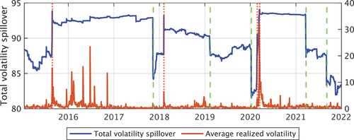
1. The China shock in 2015,

2. The Dow Jones Industrial Average (DJI) drop in 2018,

3. The COVID-19 in 2020.

Then, we can find that the time-varying spillover skyrockets at the same time as the burst events,

1. On August 25, 2015 (the China shock),

2. On February 6, 2018 (the DJI drop),

3. On February 25, and March 13, 2020 (the COVID-19).

In most cases, we cannot understand the reason for the decrease in the spillovers. However, the reason for the fourth decrease on 22 March 2021 is clear. The state of emergency in Japan ended on 21 March 2021, and we can consider that the market judged the COVID-19 to be over. This fact is confirmed that the time-varying volatility spillover did not increase when the state of emergency was declared again a month later. As shown in this figure, the total spillover index among Japanese industrial sectors varies over time, indicating that investors can frequently revise their portfolios (Mensi et al., 2021). See SM for details on volatility spillovers between individual sectors in the TOPIX-17 series between the pre- and post-COVID-19 periods.

4.3. Portfolio strategy

Although many papers indicate that investigating the time-varying volatility spillover is useful for investors, they do not mention how to use the time-varying volatility spillover. Thus, we analyze that a portfolio reallocation based on the time-varying volatility spillover using an extremely simple method, which is more effective than a periodic reallocation. First, we show two time-varying portfolio weight series where one is allocated daily, and the other is based on the increase or decrease time-varying volatility spillover, which means that the portfolio weight is reallocated when the time-varying volatility spillover increases or decreases. These two time-varying weight series are called daily weight and spillover weight. Second, using the cumulative return and the Sharpe ratio, we confirm how effective the spillover weight is.

4.3.1. Portfolio weight

We calculate the minimum variance portfolio weight $w_t$ as follows:

${\omega }_t=\frac{{\mathrm{\Sigma }}^{-1}1}{1^{\prime }{\mathrm{\Sigma }}^{-1}1},$

where ${\mathrm{\Sigma }}^{-1}$ is a sample inverse covariance matrix that is estimated by closing prices within 250 days, and 1 is a length $N$ vector with all elements being 1.

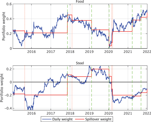
Figure 2 shows the daily weight in the blue line and the spillover weight in the red line. The spillover weight is reallocated on the next day when the volatility spillover increases or decreases. When the volatility spillover increases, the volatility in the market increases, as shown in Figure 1. As shown in Figure 2, the daily weight vastly changes when the volatility spillover increases or decreases. This technique achieves a more accurate and timely reallocation, as stated by Ahmad et al. (2021). The spillover weight can also capture the fluctuation of the daily weight and curb the number of reallocations.

Figure 2. The time-varying portfolio weight of the food and steel sectors. The blue line is reallocated every day, and the red line is reallocated depending on the increase or decrease of the volatility spillover.

4.3.2. Effectiveness

To evaluate the effectiveness of the spillover weight, we compare the cumulative returns and the Sharpe ratio among the equal, daily, weekly, monthly, yearly, and spillover weights. When the returns are calculated, we consider transaction costs. The portfolio returns $r_{pt}$ are calculated by subtracting the transaction cost $c$ incurred by the reallocation as follows:

$\mathrm{T}{\mathrm{O}}_t=\sum _{n=1}^N\left|{\omega }_t^{(n)}-{\omega }_{t-1}^{(n)}\right|,r_{pt}={\omega }_t^{\prime }{r}_t-c\mathrm{T}{\mathrm{O}}_t,$

where ${\omega }_t^{(n)}$ and $r_t^{(n)}$ are the portfolio weight and return of $n$-th stocks at $t$. Additionally, the transaction cost $c$ is set as 0,1,5,10,20,50 bp. The calculation of $\mathrm{T}{\mathrm{O}}_t$ is inspired by Paolella et al. (2021). However, we consider only the difference between portfolio weights at $t$ and $t-1$.

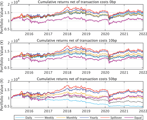
Figure 3 shows the cumulative returns with $c=0,10,50$ bp. When $c=0,10$ bp, all portfolios outperform the equal weight. When $c=50$ bp, the cumulative returns of the daily and weekly portfolios are not only less than the equal weight portfolio but also negative because of high transaction costs. However, despite the heavy transaction costs, the yearly and spillover portfolios’ returns are larger than the equal weight portfolio. Notably, the spillover weight portfolio generates the highest cumulative returns.

Figure 3. Cumulative returns net of three types of transaction costs with an initial value of ¥ 10,000. The spillover weight portfolio is based on the increase and decrease in the volatility spillover.

Then, we compare portfolios with the Sharpe ratio. Table 2 shows all Sharpe ratios for each reallocation interval and the number of reallocations. We find that the value of spillover weight is the best among all portfolios and all transaction costs. Even though the spillover weight portfolio has been reallocated more often than the yearly weight portfolio, it has a larger Sharpe ratio and greater cumulative returns.

Table 2. Sharpe ratio of each portfolio and each transaction cost

	0 bp	1 bp	5 bp	10 bp	20 bp	50 bp	Times
Daily	0.0239	0.0226	0.0173	0.0107	−0.0025	−0.0418	1704
Weekly	0.0189	0.0183	0.0158	0.0126	0.0062	−0.0129	341
Monthly	0.0201	0.0198	0.0184	0.0167	0.0132	0.0029	78
Yearly	0.0244	0.0243	0.0238	0.0232	0.0219	0.0182	7
Spillover	0.0273	0.0271	0.0266	0.0260	0.0247	0.0208	9
Equal	0.0096	0.0096	0.0096	0.0096	0.0096	0.0096	0

Notes: The bp means 0.01%, and Times is the number of reallocations.

To investigate in detail, we consider two portfolios: one is reallocated depending on the increase spillover effect/timing, and the other is reallocated depending on the decrease spillover effect/timing. Figures 4 and 5 show the cumulative returns based on the increase and decrease spillover, respectively. Hereafter, each portfolio is called the increased spillover weight portfolio and the decreased spillover weight portfolio. In Figure 4, the increased spillover weight portfolio has the highest returns, the same as in Figure 3. However, the decreased spillover weight portfolio makes lower returns than other portfolios without a transaction costs, and it is worse than the yearly portfolio with 10 and 50 bp transaction costs. Finally, we compare the Sharpe ratio in three spillover weight portfolios in Tables 2 and 3. The value of the increased spillover weight portfolio is the best of the three spillover weight portfolios. However, the value of the decreased spillover weight is not only the lowest of the three spillover weight portfolios but also it is lower than some periodic portfolios when a transaction costs are low.

Figure 4. Cumulative returns net of three types of transaction costs with an initial value of ¥ 10,000. The spillover weight portfolio is based on the increase in the volatility spillover.

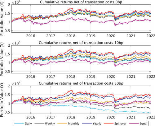
Figure 5. Cumulative returns net of three types of transaction costs with an initial value of ¥ 10,000. The spillover weight portfolio is based on the decrease in the volatility spillover.

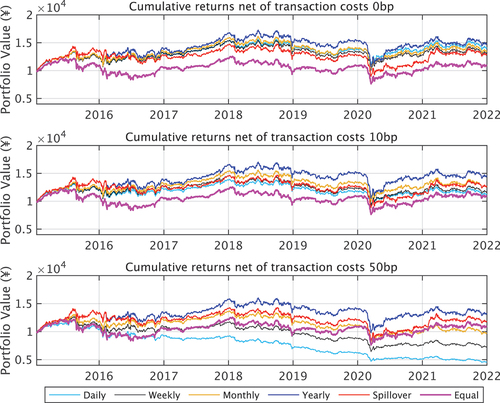
Table 3. Sharpe ratio of two spillover weight portfolios depending on the increase and the decrease in the volatility spillover

	0 bp	1 bp	5 bp	10 bp	20 bp	50 bp	Times
Spillover (increase)	0.0281	0.0280	0.0277	0.0272	0.0263	0.0236	4
Spillover (decrease)	0.0172	0.0171	0.0168	0.0163	0.0154	0.0128	5

Notes: The bp means 0.01% and Times is the number of reallocations.

From the relationship between the time-varying volatility spillover and portfolio strategies, we can say that we should at least pay attention to the increase volatility spillover.

4.4. Robustness checks

Our results in Section 4.3.2 show not only the effectiveness of the reallocation based on the volatility spillover but also that the wrong timing of the reallocation could cause a lower return. Therefore, in this section, we consider several orders ($p$), window sizes ($\omega$), and forecast error horizons ($H$) to check the robustness of our results. To do that, we use the VAR model with the following parameter sets: $p=1,2,$ and 3; $\omega =200,250,$ and 300; and $H=3,5,$ and 10.

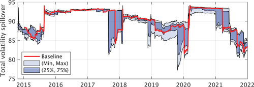
Figure 6 presents the time-varying total volatility spillover based on each combination. The red line in this figure shows the baseline spillover whose order, window size, and forecast error horizon are $p=2$, $\omega =250$, and $H=5$. The light blue area shows from the minimum to the maximum value, and the dark blue area denotes the 25% and 75% quantiles in this figure. We can find that when the time-varying spillover is large, the range of estimation is small; when the time-varying spillover is small or close to decreasing, the range of estimation becomes wide. In addition, although the sharp increase of the time-varying spillover when the China shock, the DJI drop, and the COVID-19 shock happened is the same time regardless of the parameters, the point of decrease of the time-varying spillover is different between a set of parameters. Therefore, when our proposed method is used, we have to change the timing of reallocation.

Figure 6. Robustness checks of time-varying spillover. The red line shows the baseline spillover whose order, window size, and forecast error horizon are $p=2$, $\omega =250$, and $H=5$, respectively. The light blue area shows from the minimum value to maximum value, and the dark blue area denotes the 25% and 75% quantiles.

Then, we confirm the robustness of our proposed method using the time-varying spillover for each parameter. Table 4 shows the Sharpe ratio calculated with each spillover weight. In this table, the underline denotes the benchmark which we use in Section 4.3.2, and the bold values are the best values among the same rolling-sample window. Additionally, as the start point of the sample period is changed when the rolling-sample window is different, we evaluate spillover weights for each rolling-window sample. As if the order and the rolling-window sample of the VAR model are the same, the obtained values are the same regardless of the forecast horizon of the forecast variance error decomposition; we report the Sharpe ratio regardless of it.

Table 4. Sharpe ratio of each portfolio and each transaction cost

	0 bp	1 bp	5 bp	10 bp	20 bp	50 bp	Times
order ($p$)	$\omega =200$
Yearly	0.0261	0.0260	0.0254	0.0247	0.0232	0.0188	7
1	0.0275	0.0273	0.0267	0.0259	0.0244	0.0196	10
2	0.0267	0.0265	0.0259	0.0250	0.0234	0.0183	10
3	0.0263	0.0261	0.0255	0.0246	0.0230	0.0178	10
order ($p$)	$\omega =250$
Yearly	0.0261	0.0260	0.0255	0.0248	0.0235	0.0195	7
1	0.0306	0.0305	0.0300	0.0293	0.0280	0.0241	9
2	0.0302	0.0300	0.0295	0.0288	0.0275	0.0233	9
3	0.0295	0.0294	0.0288	0.0281	0.0268	0.0226	9
order ($p$)	$\omega =300$
Yearly	0.0101	0.0099	0.0095	0.0089	0.0078	0.0043	7
1	0.0173	0.0171	0.0167	0.0161	0.0150	0.0117	8
2	0.0176	0.0175	0.0170	0.0164	0.0153	0.0118	8
3	0.0176	0.0175	0.0171	0.0165	0.0153	0.0118	8

Notes: The order ($p$) denotes the order of each VAR model, and $\omega$ is the rolling-sample window and the sample size of sample covariance matrixes. The underline denotes the benchmark we used in Section 4.3.2, and the bold values are the best values among same rolling-sample window $\omega$.

At first, we confirm the result of $\omega =200$. When we use the strategy based on the time-varying spillover calculated by the VAR(1) model, the best Sharpe ratio can be obtained. For other orders, $p=2$ and 3, there are some fewer values than the yearly portfolio depending on the transaction cost. Then, for $\omega =250$, while this rolling-window sample includes the benchmark, the best case is the $p=1$ similar to $\omega =200$. The difference point from $\omega =200$ is that the Sharpe ratio is larger than that of the yearly portfolio for all patterns, no matter which order and transaction cost is chosen. Finally, we confirm the $\omega =300$. Unlike $\omega =200,250$, the VAR(3) model is the best. However, since there are no large differences between other orders, we can consider that if we have a sufficient sample size to estimate models, the effect of the change, depending on the order, is small.

To confirm robustness for types of portfolio, we make other portfolios, the minimum variance portfolio, and the mean-variance portfolio without short position.³ For the mean-variance portfolio, we set that the expected return is the sample mean of asset returns during whole samples, and we adopt the weight which makes a portfolio maximize its Sharpe ratio. Table 5 shows the Sharpe ratio of minimum variance and mean-variance portfolios without a short position. Similar to the minimum variance portfolio, the spillover portfolios can generate the largest Sharpe ratio. Especially for the mean-variance portfolio, although all periodic portfolios show a similar value when the transaction cost is small, the spillover portfolio has greater value.

Table 5. Sharpe ratio of minimum variance and mean-variance portfolios without short position

	0 bp	1 bp	5 bp	10 bp	20 bp	50 bp
Minimum variance without short
Daily	0.0121	0.0117	0.0102	0.0084	0.0048	−0.0062
Weekly	0.0098	0.0096	0.0089	0.0079	0.0061	0.0004
Monthly	0.0094	0.0093	0.0088	0.0083	0.0073	0.0042
Yearly	0.0138	0.0137	0.0136	0.0134	0.0130	0.0119
Spillover	0.0152	0.0152	0.0150	0.0148	0.0143	0.0130
Mean-variance without short
Daily	0.0344	0.0343	0.0339	0.0334	0.0323	0.0293
Weekly	0.0343	0.0342	0.0340	0.0337	0.0331	0.0313
Monthly	0.0346	0.0345	0.0344	0.0342	0.0338	0.0327
Yearly	0.0340	0.0340	0.0339	0.0339	0.0337	0.0334
Spillover	0.0365	0.0365	0.0364	0.0363	0.0361	0.0356

Notes: The bp means 0.01%, and Times is the number of reallocations.

5. Discussion

Studying cross-sector information contagion is essential for understanding risk behavior and optimal portfolio allocation. According to the study on economic uncertainty during COVID-19 by Castelnuovo (2022, p.30), “Recent contributions have tried to isolate the role of sectoral uncertainty to have a better understanding on which sectors are mostly responsible for the negative business cycle effects of uncertainty shocks.” In practice, investment concerning the industrial sector is even more significant. For example, an article on investopedia.com by Adam Hayes (updated 22 June 2022) stated, “Sector ETFs have become popular among investors and can be used for hedging and speculating”.⁴ Thus, our research motivation is to construct an optimal portfolio that considers cross-sector information contagion. As for the latest research on this topic, the following studies have been published. S. Y. Choi (2022) investigated the volatility spillovers among various industries during the COVID-19 pandemic, whereas Mahran (2022) employed the DCC-GARCH model to examine volatility connectedness in a sample of 10 sectors in the Egyptian stock market. Moreover, Malik (2022) focused on volatility spillover among major U.S. equity sectors by using daily data with bivariate GARCH models.

Several recent studies have analyzed the relationship between volatility spillover and portfolio optimization. In addition to the papers discussed in the Introduction, the most recent studies, such as Konstantinov and Fabozzi (2022), in their estimation of portfolio volatilities, used variance-decomposition techniques and Cholesky factorization to construct a portfolio volatility spillover index. Shi and Zhou (2022) employed the generalized forecast error variance decomposition based on a vector autoregression model to investigate factors’ volatility spillovers. Using the TVP-VAR model, Furuoka et al. (2023) examined energy and agricultural commodities’ short- and long-term connectedness. J. Liu et al. (2023) used the DCC-MVGARCH model and spillover index method to investigate volatility linkages between the European carbon emissions and energy markets. Yadav et al. (2023) examined the volatility spillover between the Chinese stock market and four emerging economies by using Granger causality and the DCC-GARCH model.

The present study combines these two aforementioned issues and proposes a direction for optimal portfolio allocation based on cross-sector information contagion. To the best of the author’s knowledge, such studies are rare. Therefore, this study presents a new and valuable technique for academia and for relevant research domains.

6. Conclusion

This paper measured the time-varying spillover among Japanese stock sectoral indices and analyzed the portfolio strategies based on cross-sector information contagion. To measure the volatility spillover, we used the spillover index proposed by Diebold and Yilmaz (2012). Since the spillover index can measure the total and directional spillover, this method is widely used. In this paper, we used only the total spillover to confirm the status of the market.

By investigating the time-varying spillover, we confirmed that the total spillover displayed a clear increase associated with easily identified crisis events such as the China shock in 2015, the DJI drop in 2018, and the COVID-19 in 2020.

We analyzed the portfolio strategies based on the time-varying spillover by implementing a strategy using the volatility spillover reallocated portfolios based on the increase or decrease in the time-varying volatility spillover. We compared this method to some periodic reallocation portfolios and showed that our approach had the most significant cumulative returns with the greatest Sharpe ratio. Furthermore, we found that investors should at least consider the increase spillover. Even though these are just a few examples of how to use the volatility spillover for portfolio reallocation, our results support the finding that the volatility spillovers are useful for investors.

This paper applies only the DY index to investment strategies. However, other spillover indices are proposed, for example, the asymmetric spillover index (Baruník et al., 2016) and the frequency domain spillover (Baruník & Křehlík, 2018), and these indices are more informative than the DY index. Therefore, we have to examine the portfolio allocation using them in the future.

Future research should investigate the effects of other financial crises in other markets. In particular, we could compute the Sharpe ratios for different crisis periods to determine if our results still hold over such periods.

Disclosure statement

No potential conflict of interest was reported by the author(s). The views expressed in this paper are those of the authors and do not necessarily reflect the official views of Nomura Holdings or Kwansei Gakuin University.

Additional information

Funding

This study is partly supported by the Institute of Statistical Mathematics (ISM) cooperative research program [2022-ISMCRP-2024], JSPS KAKENHI [Grant Number 21K01433], and Grant-in-Aid for JSPS Fellows [Grant Number 22J10285].

Notes

1. The TOPIX-17 series is a stock price index that reorganizes the TOPIX (traditionally used to classify Japanese stocks) into 17 industries for investment convenience.

2. MFE Toolbox: https://www.kevinsheppard.com/MFE_Toolbox

3. Since results depend on the lower bound of a short position, we do not consider the mean-variance portfolio with a short position.

4. See https://www.investopedia.com/terms/s/sector-etf.asp.

References

- Ahmad, W., Hernandez, J. A., Saini, S., & Mishra, R. K. (2021). The US equity sectors, implied volatilities, and COVID-19: What does the spillover analysis reveal? Resources Policy, 72, 102102. https://doi.org/10.1016/j.resourpol.2021.102102
- Akhtaruzzaman, M., Boubaker, S., & Sensoy, A. (2020). Financial contagion during COVID–19 crisis. Finance Research Letters, 38, 101604. https://doi.org/10.1016/j.frl.2020.101604
- Andersen, T. G., & Bollerslev, T. (1998). Answering the skeptics: Yes, standard volatility models do provide accurate forecasts. International Economic Review, 39(4), 885–13. https://doi.org/10.2307/2527343
- Baruník, J., Kočenda, E., & Vácha, L. (2016). Asymmetric connectedness on the U.S. stock market: Bad and good volatility spillovers. Journal of Financial Markets, 27, 55–78. https://doi.org/10.1016/j.finmar.2015.09.003
- Baruník, J., & Křehlík, T. (2018). Measuring the frequency dynamics of financial connectedness and systemic risk. Journal of Financial Econometrics, 16(2), 271–296. https://doi.org/10.1093/jjfinec/nby001
- Castelnuovo, E. (2022). Uncertainty before and during COVID-19: A survey. Journal of Economic Surveys, 37(3), 821–864. https://doi.org/10.1111/joes.12515
- Choi, S. Y. (2022). Dynamic volatility spillovers between industries in the US stock market: Evidence from the COVID-19 pandemic and black monday. The North American Journal of Economics & Finance, 59, 101614. https://doi.org/10.1016/j.najef.2021.101614
- Choi, K. H., McIver, R. P., Ferraro, S., Xu, L., & Kang, S. H. (2021). Dynamic volatility spillover and network connectedness across ASX sector markets. Journal of Economics & Finance, 45(4), 677–691. https://doi.org/10.1007/s12197-021-09544-w
- Costa, A., Matos, P., & da Silva, C. (2021). Sectoral connectedness: New evidence from US stock market during COVID-19 pandemics. Finance Research Letters, 102124. https://doi.org/10.2139/ssrn.3805087
- Diebold, F. X., & Yilmaz, K. (2009). Measuring financial asset return and volatility spillovers, with application to global equity markets. The Economic Journal, 119(534), 158–171. https://doi.org/10.1111/j.1468-0297.2008.02208.x
- Diebold, F. X., & Yilmaz, K. (2012). Better to give than to receive: Predictive directional measurement of volatility spillovers. International Journal of Forecasting, 28(1), 57–66. https://doi.org/10.1016/j.ijforecast.2011.02.006
- Diebold, F. X., & Yilmaz, K. (2014). On the network topology of variance decompositions: Measuring the connectedness of financial firms. Journal of Econometrics, 182(1), 119–134. https://doi.org/10.1016/j.jeconom.2014.04.012
- Fasanya, I. O., Oyewole, O., Adekoya, O. B., & Odei-Mensah, J. (2021). Dynamic spillovers and connectedness between COVID-19 pandemic and global foreign exchange markets. Economic Research-Ekonomska Istrazivanja, 34(1), 2059–2084. https://doi.org/10.1080/1331677X.2020.1860796
- Furuoka, F., Yaya, O. O. S., Ling, P. K., Saleh Al-Faryan, M. A., & Islam, M. N. (2023). Transmission of risks between energy and agricultural commodities: Frequency time-varying VAR, asymmetry and portfolio management. Resources Policy, 81, 103339. https://doi.org/10.1016/j.resourpol.2023.103339
- Konstantinov, G. S., & Fabozzi, F. J. Portfolio volatility spillover. (2022). International Journal of Theoretical and Applied Finance, 25(4n05), 2250019. https://doi.org/10.1142/S0219024922500194
- Koop, G., Pesaran, M. H., & Potter, S. M. (1996). Impulse response analysis in nonlinear multivariate models. Journal of Econometrics, 74(1), 119–147. https://doi.org/10.1016/0304-4076(95)01753-4
- Laborda, R., & Olmo, J. (2021). Volatility spillover between economic sectors in financial crisis prediction: Evidence spanning the great financial crisis and Covid-19 pandemic. Research in International Business and Finance, 57, 101402. https://doi.org/10.1016/j.ribaf.2021.101402
- Liu, J., Hu, Y., Yan, L. Z., & Chang, C. P. (2023). Volatility spillover and hedging strategies between the European carbon emissions and energy markets. Energy Strategy Reviews, 46, 101058. https://doi.org/10.1016/j.esr.2023.101058
- Liu, Y. A., & Pan, M.-S. (1997). Mean and volatility spillover effects in the U.S. and Pacific–Basin stock markets. Multinational Finance Journal, 1(1), 47–62. https://doi.org/10.17578/1-1-3
- Liu, Y., Wei, Y., Wang, Q., & Liu, Y. International stock market risk contagion during the COVID-19 pandemic. (2022). Finance Research Letters, 45(February), 102145. https://doi.org/10.1016/j.frl.2021.102145
- Mahran, H. A. (2022). The impact of the Russia–Ukraine conflict (2022) on volatility connectedness between the Egyptian stock market sectors: Evidence from the DCC-GARCH-CONNECTEDNESS approach. The Journal of Risk Finance, 24(1), 105–121. https://doi.org/10.1108/JRF-06-2022-0163
- Malik, F. Volatility spillover among sector equity returns under structural breaks. (2022). Review of Quantitative Finance & Accounting, 58(3), 1063–1080. https://doi.org/10.1007/s11156-021-01018-8
- Mensi, W., Nekhili, R., Vo, X. V., Suleman, T., & Kang, S. H. (2021). Asymmetric volatility connectedness among U.S. stock sectors. The North American Journal of Economics & Finance, 56, 101327. https://doi.org/10.1016/j.najef.2020.101327
- Paolella, M. S., Polak, P., & Walker, P. S. (2021). A non-elliptical orthogonal GARCH model for portfolio selection under transaction costs. Journal of Banking and Finance, 125(106046). https://doi.org/10.1016/j.jbankfin.2021.106046.
- Pesaran, H. H., & Shin, Y. (1998). Generalized impulse response analysis in linear multivariate models. Economics Letters, 58(1), 17–29. https://doi.org/10.1016/s0165-1765(97)00214-0
- Shahzad, S. J. H., Naeem, M. A., Peng, Z., & Bouri, E. (2021). Asymmetric volatility spillover among Chinese sectors during COVID-19. International Review of Financial Analysis, 75(April), 101754. https://doi.org/10.1016/j.irfa.2021.101754
- Shigemoto, H., & Morimoto, T. (2022). Volatility spillover among Japanese sectors in response to COVID-19. Journal of Risk and Financial Management, 15(10), 480. https://doi.org/10.3390/jrfm15100480
- Shi, H. L., & Zhou, W. X. (2022, March). Factor volatility spillover and its implications on factor premia. Journal of International Financial Markets, Institutions and Money, 80, 101631. https://doi.org/10.1016/j.intfin.2022.101631
- Sultonov, M. (2021). External shocks and volatility overflow among the exchange rate of the Yen, Nikkei, TOPIX and sectoral stock indices. Journal of Risk and Financial Management, 14(11), 560. https://doi.org/10.3390/jrfm14110560
- Wang, G. J., Xie, C., Jiang, Z. Q., & Eugene Stanley, H. (2016). Who are the net senders and recipients of volatility spillovers in China’s financial markets?. Finance Research Letters, 18(11), 255–262. https://doi.org/10.1016/j.frl.2016.04.025
- Yadav, M. P., Sharma, S., & Bhardwaj, I. (2023). Volatility spillover between Chinese stock market and selected emerging economies: A dynamic conditional correlation and portfolio optimization perspective. Asia- Pacific Financial Markets, 30(2), 427–444. https://doi.org/10.1007/s10690-022-09381-9
- Yilmaz, K. (2010). Return and volatility spillovers among the East Asian equity markets. Journal of Asian Economics, 21 (3), 304–313. http://doi.org/10.1016/j.asieco.2009.09.001