Structural and stochastic poverty, shocks, and resilience capacity in rural Ethiopia

Abstract

Whilst structurally poor households fall below the income and asset poverty line, stochastically poor households fall below the income poverty line but above the asset poverty line. This distinction suggests different challenges for the households in dealing with shocks and building the resilience to make a lasting escape from poverty. Accordingly, we examine the effect of shocks on structural and stochastic poverty, transitions, and the role of resilience as a mechanism for dealing with shocks and stochastic and structural poverty using the Ethiopian Socioeconomic Survey data. We find that recurrent and concurrent shocks adversely impact structural and stochastic poverty, whilst resilience capacities can curb poverty as shocks intensify. Access to irrigation, literacy, good vegetation cover, and non-farm economic activities help eradicate both structural and stochastic poverty. Rainfall variability, drought, conflict, input and output price volatility, and idiosyncratic shocks all drive both structural and stochastic poverty. However, the critical implication for policy is that reducing structural and stochastic poverty requires enhancing resilience capacity. This will require promoting symbiotic rural–urban links and rural revitalization to ensure a balanced mix of development. The findings suggest that two distinct sets of policies are required to protect against falling into poverty and sustain movements out of poverty, namely harmonizing cargo net and safety net policies.

Keywords:

• shocks
• poverty
• cox proportional hazard
• panel data
• rural Ethiopia

PUBLIC INTEREST STATEMENT

Stochastic events in Ethiopia are the worst setback in poverty reduction. Relief efforts are aimed to respond to crises by protecting the life and livelihoods after a shock. As such, these interventions deal for a large part with coping strategies and trying to strengthen the absorptive capacity.. In contrast, development efforts mostly aimed at addressing long-term issues of societal changes and deal with incremental adjustment and transformational changes. Resilience is introduced to transcend the pitfalls of earlier interventions. “An ounce of prevention is worth a proud of cure” - Economics of resilience. Despite its added-value, resilience needs to be embodied in a more rigorous empirical analysis. To design appropriate poverty reduction policies, reformulating poverty analysis toward the third-generation measures (structural and stochastic) is overwhelming. The empirics also underscore the need for a forward-looking and dynamic framework that consistently predicts future poverty. This paper examines how resilience mediates the relationship between shocks and structural and stochastic poverty.

1. Introduction

The national development plans and strategies that Ethiopia has implemented to reduce poverty have made notable achievements. In particular, the country’s steady economic performance facilitated a decline in monetary poverty by 21%, from 29.6% to 23.5% and enabled 2.3 million people to escape poverty between 2011/12 and 2015/16 (World Bank, 2020). Nevertheless, Ethiopia is registered to be the poorest in Sub Sahara Africa having a multidimensional poverty index of 0.687 (OPHI, 2019). Poverty will remain a major challenge in the country for decades to come (Stifel and Woldehanna, 2017; Swanepoel, 2005; World Bank, 2015).

Economic growth in Ethiopia over the past two decades has not been trickled down to the rural population. Moreover, poverty reduction has also been setback by specific challenges, particularly those arising from shocks in the economy. The current bloody civil war has cost hundreds of thousands of lives, millions have been displaced, and many are in desperate need of assistance. The war also incurs a huge material cost and has battered the economy. Ethiopia, like every economy, has also been adversely impacted by the COVID-19 pandemic and a combination of shocks arising from the Russia-Ukraine war and the effects of the global downturn which have hit the economy and exacerbated poverty (Abebaw et al., 2020; Habtewold, 2021). Ethiopia also experiences high inflation, unemployment, low wages (CEPHEUS, 2020), rising sociopolitical instability, poor access to basic services, land tenure insecurity, weak capital accumulation, and environmental (Bekele, 2018).

Smallholders are subjected to covariate and idiosyncratic shocks. Covariate shocks affect all households in the village and possibly those nearby, whereas shocks in which the impacts are limited to the individual or household levels are idiosyncratic (Pradhan & Mukherjee, 2018). These include, for example, climate-related (Hirvonen et al., 2020), price-related (Hill & Porter, 2017), and health-related (Gebremariam & Nd Tesfaye, 2018) shocks that intensified poverty by reducing education participation, labor market participation, and agricultural output, subsequently driving a decline in incomes and consumption (Ngoma et al., 2019). Shocks undermine the ability of households to develop stocks of wealth and prevent them from using those stocks effectively. When prolonged, shocks result in a downward spiral of asset loss (Barua & Banerjee, 2020). The recurrence and concurrence of shocks wipe out livelihood resources and work against efforts to eradicate poverty (Campos et al., 2014). The poverty trajectories of households typically include periods of rising and falling fortunes (Krishna & Krishna, 2017) such that gains often prove transitory, and it is difficult for poor households to achieve a lasting reversal of fortune (Mariotti & Diwakar, 2016).

Ethiopia’s official poverty statistics follow the conventional approach (MoFED, 2012, 2017). However, this approach has methodological flaws and has been strongly criticized for its inability to capture multifaceted attributes (Krishna & Krishna, 2017). This approach does not engage with the way that consumption expenditure tends to fluctuate over time (Hulme & Shepherd, 2003) nor does it take into account inequalities in intrahousehold resource allocation (Tran et al., 2014).

The national poverty reduction strategies function in silos polarized around relief and development and lack systematic attempts to identify those who are in need, to determine what their needs are, or to address them in a way that would enable them to sustain an escape from poverty. These standardized national policy and strategies have little room to engage with the multifaceted character of poverty. However, it is imperative that this mosaic of development and humanitarian efforts becomes more integrated to support more households to make lasting movements out of poverty. Thinking about how to integrate relief and development has been organized around the idea of resilience. A resilience lens argues for bringing together preemptive and redemptive policies in the fight against poverty (Barrett, 2005; Sou, 2019). Despite its claim to add value to poverty reduction policies, resilience has (yet) to be embodied in a more rigorous empirical analysis.

Reformulating poverty analysis toward third-generation measures has long been the interest of development research. A hallmark of integrated modeling is striving to improve precision in measuring structural and stochastic poverty (Radeny et al., 2012, Carter & Barrett, 2006; Schotte, 2019). A few empirical studies underscore the claim that shocks perpetuate monetary poverty (Barua & Banerjee, 2020; Brück & Workneh Kebede, 2013; Shehu & Sidique, 2020). Other studies statically quantify the effect of shocks on structural and stochastic poverty (Angelsen & Dokken, 2018; Ngoma et al., 2019). Thus far, the literature lacks rigorous empirical analyses on the linkages among shocks, resilience, and structural and stochastic poverty. Against this backdrop, this study sheds light on the effect of shocks on structural and stochastic poverty and the role of resilience as a mechanism for dealing with shocks and structural and stochastic poverty. It also scrutinizes how shocks, resilience, and other covariates prompt simultaneous ebbs and grows in structural and stochastic poverty in rural Ethiopia. Our starting point here is that an explanation of overall poverty trends needs more fine-grained insights into both movements out of and into poverty in order to understand how some (and not others) are able to sustain their escape from poverty.

The paper is structured as follows: Section 2 presents the theoretical framework. In section 3, we briefly discuss the research methodologies. Section 4 discusses the major results. Finally, section 5 concludes the paper.

2. Theoretical framework

In the wake of liquidity constraints, the notion that poor households will smooth consumption has a firm theoretical foundation. Carter and Lybbert (2012) also acknowledged that the poor often prefer to smooth their consumption rather than their assets in the event of shocks. The possible reason is that selling productive assets would induce a permanent income loss for a household, which would subsequently leave them trapped in poverty. To obtain a clear insight into drivers and interrupters of structural and stochastic poverty and the mediating role of resilience between shocks and structural and stochastic poverty, this paper follows the asset smoothing approach of Carter and May (1999). The approach underlines the role of productive assets in enhancing the income-generating process and serving as a buffer stock in times of an anticipated decline in income. In other words, the sustainable welfare implications of asset smoothing could well be an intergenerational asset transfer that could shield ensuing generations, as well as the current generation, from poverty.

The implication is that if assets can be maintained by reducing income temporarily in the face of a shock, then households may be able to weather shocks without compromising their potential to escape poverty—in other words, asset-smoothing is a resilience capacity. Resilience here is the capacity to hold productive asset stock above a minimum critical asset poverty threshold over time. Therefore, increasing resilience means increasing the probability of holding assets above the critical threshold (Phadera et al., 2019). These capacities protect households from poverty in the presence of shocks. Reformulating poverty analyses using the third-generation measures can help us understand the more forward-looking question of who is likely to remain poor into the future. This implies that we need to distinguish more carefully between changing income levels and asset levels in the face of shocks to better understand poverty transitions. Since poverty is dynamic, certain subgroups are more likely than others to remain poor in the long run. Therefore, it is important to move beyond poverty headcount to the analyses of structural and stochastic forms of transitory and chronic poverty through an asset-based disaggregation of expected welfare (Carter and Barrett, 2006).

Figure 1 schematically depicts how asset accumulation and income decompose different types of poverty. The axes measure the income of the households (vertical) and assets accessible to households (horizontal). Likewise, the vertical and horizontal grid lines represent income and asset poverty lines. The income poverty line (Z) categorizes households as poor and non-poor typically measured by estimating whether a household has enough income, or consumes enough, to surpass some social definition of basic needs. The asset poverty line ($\bar{\mathrm{A}}$) entails the level of assets that are expected to yield income equal to the poverty line. The line divides the asset poor and non-poor (Carter & May, 1999). Based on the value of income (Y_i), the asset poverty indexes (API), the income poverty line (Z), and the asset poverty line ($\bar{\mathrm{A}}$), we can identify the structural and stochastically poor as follows. Structurally poor households’ inability to secure income or assets above the poverty line further reinforces their poverty making it more likely to be chronic and persistent. Structurally poor households are located at point D: their realized income is below the income poverty line (${\mathrm{Y}}_{\mathrm{i}}<\mathrm{Z}$) and their assets are below the asset poverty line ($\mathrm{A}\mathrm{P}{\mathrm{I}}_{\mathrm{i}}<\bar{\mathrm{A}}$). Although stochastically poor households’ income falls below the poverty line, they maintain their assets above the poverty line and in this way shield themselves from becoming structurally poor, enabling them to climb out of poverty when their income improves. Stochastically poor households are located at point A: their realized income is below the income poverty line (${\mathrm{Y}}_{\mathrm{i}}<\mathrm{Z}$) but their assets are above the asset poverty line ($\mathrm{A}\mathrm{P}{\mathrm{I}}_{\mathrm{i}}>\bar{\mathrm{A}}$). It is also possible for a household to be income non-poor $({\mathrm{Y}}_{\mathrm{i}}>\mathrm{Z})\hspace{0.17em}$but asset-poor$\hspace{0.17em}(\mathrm{A}\mathrm{P}{\mathrm{I}}_{\mathrm{i}}<\bar{\mathrm{A}})$. These households are stochastically non-poor and are located at point B. Finally, households positioned at point C are structurally non-poor households (being neither income (${\mathrm{Y}}_{\mathrm{i}}<Z$) nor asset ($\mathrm{A}\mathrm{P}{\mathrm{I}}_{\mathrm{i}}>\bar{\mathrm{A}}$) poor).

Figure 1. Integrated measures of poverty (Carter & May, 1999).

According to Carter and Barrett (2006) household movements into and out of poverty may represent distinctive experiences of poverty transitions. Crucially, third-generation poverty analysis examines the degree to which transitions are stochastic or structural. Movements out of poverty during a given period are stochastic—represented on Figure 1 by either a movement from being stochastically poor (A) to being structurally non-poor (C) or from being structurally poor (D) to stochastically non-poor (B)—or whether they structural—a movement from being structurally poor (D) to structurally non-poor (C) (Dutta, 2021). Similarly, movements into poverty in a given period are either stochastic—represented on Figure 1 by a movement either from being stochastically non-poor (B) to structurally poor (D) or from being structurally non-poor (C) to being stochastically poor (A)—or structural—a movement from being structurally nonpoor (C) to structurally poor (D).

Stochastic poverty transitions may be the result of a temporary spell of good luck, a successful new strategy, or recovery from an episode of bad luck episode. It is well recognized, for instance, that taking on wage income is one of the diversified strategies that many stochastically non-poor have pursued to successfully escape poverty. Structural poverty transitions could result from the accumulation of new assets or enhanced returns to assets already possessed.

In decomposing poverty transitions, there are also always poor and never poor households. Some of these households may have moved between stochastically poor/non-poor and structurally poor/non-poor categories but such movements do not represent transitions in or out of poverty, even though they may be significant for the future possibility of moving into or out of poverty. Households that remain poor during a given period, whether due to structural poverty or negative shocks, are designated as being chronically poor whilst those that remain non-poor during a given period, whether due to their structural position or positive shocks, are designated as the never poor.

3. Material and methods

3.1. Data

The study uses the three rounds of the Ethiopian Socioeconomic Survey (ESS) data (2011/12–2015/16). The first wave covered only rural and small towns while expanding to urban areas in the subsequent waves. It is a rich multitopic data set consisting of detailed household information on living conditions, demographics, income, expenditure, occupation, health, education, production, asset holding, saving, and other individual and level variables. The community data entail social networks, mobility, religious practices, land use, road and market access, transport, development interventions, and business activities. It also encompasses geo-referenced variables, livestock and crop production, post-harvest, and post-planting. The sample was drawn using stratified two-stage sampling procedures.¹ We restricted our analysis to a nationally representative balanced sample of 2170 rural households because we imposed exclusion criteria such as missing information in the major variables of interests, loss due to attrition, and being unmatched in all rounds.

3.2. Shocks measures

Several shocks have been experienced in different parts of Ethiopia for the study period. Shocks are reported in response to whether the household is affected in the 12 months of the survey year. The shock variables are mostly taken as dichotomous, having values of 1 for households experiencing shocks and 0 otherwise. However, the production shock variable is aggregated from crop damage and livestock loss incidences. Likewise, the household-level shock module reports the incidence of input price, food price hikes, and food price declines, and these responses are combined to construct the price shock variable.

3.3. Resilience capacity measures

Though relatively new in development studies, resilience has the earliest root in engineering. In the 1940s and 1950s the concept emerged in psychology in the context of the adverse effects of such life events as exclusion, poverty, and traumatic stressors on vulnerable individuals, more specifically, children (Berkes & Ross, 2013). Gradually, it was popularized in ecology by a seminal work of Holling (1973) to describe the amount of disturbance a system can absorb before shifting to an alternative state. A wave of research that has moved into socio-ecological systems flooded the literature in the later decades (Folke, 2006). Resilience has been defined from a socio-ecological perspective as the capacity of socioeconomic systems to withstand shocks through absorption, adaptation, and transformation (Béné et al., 2014). Holling’s work has also become popular in several related disciplines, including disaster risk reduction (IFRC, 2016), climate change adaptation (Moser et al., 2010), social protection, and human development (Davies et al., 2013). All share an emphasis on resilience as the capacity that ensures stressors and shocks do not have long-lasting adverse development consequences (Barrett & Constas, 2014; RM-TWG, 2014).

We find that the methodologies for measuring resilience have witnessed a clear evolution. Béné et al. (2016) theory-based empirical approaches extended the methodological frontier in resilience measurements. They introduced a more elaborated conceptualization of resilience as comprising a blend of absorptive, adaptive, and transformative capacities, each of which leads to different short- and long-term responses depending on the intensity of shocks. We adopted the two stages of Principal Component Analysis (PCA) and Treelet Transformation (TT) to compute resilience capacity (RCI). PCA is employed to measure each resilience attribute (access to basic services (ABS), assets (AST), adaptive capacity (AC), and social safety net (AC) taking variables driven on an ad-hoc basis. In measuring the latent pillars, the variables (see Table 1 in the APPENDIX for details of the RIMA pillars) were selected based on the factor loadings and other statistical criteria. The Kaiser–Meyer–Olkin (KMO) measure of sampling adequacy is more than 0.60.

Table 1. Temporal distributions

	2011/12	2013/14		Change rate $\mathrm{\Delta }\left(\mathrm{\%}\right)$
			2015/16	A	B	C
Structural poor	425(18.0)	418(17.7)	475(20.1)	−0.3	2.4	2.1
Stochastic poor	597 (25.2)	579(24.5)	604(25.5)	−0.8	1.1	0.3
Stochastic non-poor	492 (20.8)	515(21.8)	572(24.2)	1.0	2.4	3.4
Structural non-poor	853 (36.0)	855(36.1)	716(30.2)	0.1	−5.9	−5.8

Notes: A = 2011/12–2013/14, B = 2013/14–2015/16, and C = 2011/12–2015/16.

In the second stage, we employed the TT data reduction technique via machine learning to compute RCI using the latent attributes. PCA is a standard dimension reduction technique that works by calculating the first few eigenvectors of a covariance and reducing the dataset to a collection of component scores. In the machine learning community, there has been a growing interest in developing alternatives to PCA that offer more interpretable components by forcing loading patterns. TT is an alternative to PCA. It introduces sparsity among component leading in an elegant fashion by combining ideas from hierarchical clustering analysis with ideas from PCA (Gorst-Rasmussen, 2012). It leads to an associated cluster tree that provides a concise visual representation of loading sparsity pattern and the general dependency structure of the data. Likewise, the novelty of TT is constructing not only clusters but also a multiresolution representation of the data (dendrogram). TT can be applied when the data are noisy, high dimensional, and unordered.

Given a collection of p observable variables, the TT algorithm entails two steps. First, we need to locate the two variables with the largest correlation coefficient. Second, these two variables have to be merged by performing PCA on them and by keeping the new variable whose score has the largest variance and leaving the residual variable. This process yields a new collection of $p-1$ variables, namely, the sum variable and the remaining $p-2$ original variables, on which we then repeat the above two steps. The variable pairing and PCA scheme is repeated for a total of $p-1$ times until only a single sum variable is left. This in turn defines a basic hierarchical clustering algorithm, the output of which is conveniently represented as a binary tree with $p$ levels (a cluster tree or cluster dendrogram). Variables that are close in this cluster tree and that are merged early represent groups of more highly correlated variables.

In measuring the latent pillars, observable variable selection is based on the factor loadings. Once each latent pillar is estimated, they are used as covariates in the construction of the RCI. Machine learning is a rapidly emerging analytical approach that attempts to build statistical models from data and make accurate predictions and decisions. TT is an unobserved type of machine learning employed for data reduction that merges hierarchical clustering with PCA.

3.4. Structural and stochastic poverty measures

This paper adopts the framework proposed by Bader et al. (2016) to integrate income and assets in constructing third-generation measures for poverty. As above, households that are income poor and lack the required assets to convert into income requirements are structurally poor. In contrast, if they obtain a level of income below the poverty line, but their asset‐based expected income level is above the asset poverty line, we identify those households as stochastically poor. Households that are non-poor by the money-metric approach but asset poor are stochastically non-poor. Those who were neither monetary nor asset poor are structurally non-poor (Dutta, 2021; Dutta & Kumar, 2015).

The income and asset poverty measures were computed as follows. Identifying the monetary poor entails choosing a welfare indicator, establishing a poverty line, and aggregating poverty data. Consumption expenditure is used since it better captures long-run welfare, reflects a household’s ability to meet its basic needs and captures households’ capabilities (World Bank, 2018). We draw the poverty line using the Cost of Basic Needs approach. Foster et al. (1984) are employed to measure monetary poverty. Let the household consumption expenditure (${\mathrm{Y}}_{\mathrm{i}}$) is ranked as:

$Y_1\le Y_2\dots \dots \dots Y_q\le \mathrm{Z}<Y_{q+1}\dots \dots \dots Y_N$

Where Z > 0 is the poverty line. The households with ${\mathrm{Y}}_{\mathrm{i}}$< Z is considered to be poor. The number of poor households is q. The cost of eliminating poverty of the i^th poor household is $\mathrm{Z}-{\mathrm{Y}}_{\mathrm{i}}$. P_α is the poverty measure, and α is the poverty aversion parameter. The Foster Greer and Thorbecke monetary poverty measures for N number of households are specified as:

$P_{\alpha }=\frac{1}{N}\sum _{i=1}^q{\left(\frac{Z-Y_i}{Z}\right)}^{\alpha };\alpha \ge 0$

For $\alpha =0$, ${\mathrm{P}}_0$ equals the headcount, which accounts for the incidence of poverty. When $\alpha =1$, ${\mathrm{P}}_1$ is the poverty gap that refers to the minimum cost of eliminating poverty. For $\alpha =2$, ${\mathrm{P}}_2$ accounts for poverty severity (Ravallion, 2016).

The asset poverty index is computed with PCA using a total of 41 assets.² The application of PCA yields a series of components, with the first component explaining the most significant variance in the data. We pooled assets across the three waves, obtained scoring factors, means, and standard deviations for the pooled data, and used the estimates to calculate period-specific asset indices. Since the data is not standardized, we ran the correlation matrix analysis to ensure that all data have equal weight. The number of principal components is extracted by selecting components where the associated eigenvalue is greater than one. We generated the index as follows:

$AP{I}_j=\sum \frac{F_i\left(X_{ji}-X_i\right)}{S_i}$

Where $\mathrm{A}\mathrm{P}{\mathrm{I}}_{\mathrm{j}}$ is the value of the j^th household’s asset poverty index, ${\mathrm{F}}_{\mathrm{i}}$ is the weight for the i^th variable, ${\mathrm{X}}_{\mathrm{j}\mathrm{i}}$ refers to the value of the i^th variable for the j^th household, and ${\mathrm{X}}_{\mathrm{i}}$ and ${\sigma }_{\mathrm{i}}$ are the mean and standard deviation of the i^th variable of the sample households. We identify the asset poverty line corresponding to a 40% headcount of monetary poverty at the population level.

3.5. Empirical strategy

3.5.1. Multinomial logit model

Since poverty in third-generation measurement is represented by four mutually exclusive categories, we can employ a discrete choice model. The multinomial logit model is often preferred when the regressors take unordered polytomous categorical variables. We estimated multinomial logit to analyze the effect of shocks on structural and stochastic poverty and the mediating role of resilience between shocks and structural and stochastic poverty. The model generates the coefficient values for three groups relative to the fourth omitted group. One of the main advantages of such an approach is the ease of specification. However, the main drawback is that it imposes the property of Independence of Irrelevant Alternatives (Wulff, 2015). Once the data fulfills this property, the model will be appropriate.

The model has four (j) equations, of which only three (j − 1) can be estimated. The multinomial logit model is identified by normalizing the coefficient of one of the categories to zero. Where ${\beta }_{\mathrm{j}}$ represents a vector of coefficients, ${\mathrm{X}}_{\mathrm{i}\mathrm{t}}$is the vector of explanatory variables, and j can take the values 0 (structural non-poor), 1 (stochastic poor), 2 (stochastic non-poor), and 3 (structural poor). To guarantee identification, ${\beta }_{\mathrm{j}}$ is set to zero for one of the categories. The structural non-poor (j = 0) is the base category. The multinomial logit model is defined as follows:

$P_{ij}=Pr\left(Y=j\right)=\frac{exp\left(X_{it}^{\prime }{\beta }_j\right)}{1+{\sum }_{j=1}^{3}exp\left(X_{it}^{\prime }{\beta }_j\right)}forj=0,1,2,3$

Setting β = 0 and computing the predicted probabilities yields:

$P_{ij}=Pr\left(Y_{it}=j|X_{it}\right)=\frac{exp\left(X_{it}^{\prime }{\beta }_j\right)}{exp\left(X_{it}^{\prime }0\right)+{\sum }_{j=1}^{3}exp\left(X_{it}^{\prime }{\beta }_j\right)}=\frac{exp\left(X_{it}^{\prime }{\beta }_j\right)}{1+{\sum }_{j=1}^{3}exp\left(X_{it}^{\prime }{\beta }_j\right)}$

And for the baseline category, we have

$P_{ij}=Pr\left(Y=0|X_{it}\right)=\frac{exp\left(X_{it}^{\prime }0\right)}{exp\left(X_{it}^{\prime }0\right)+{\sum }_{j=1}^{3}exp\left(X_{it}^{\prime }{\beta }_j\right)}=\frac{1}{1+{\sum }_{j=1}^{3}exp\left(X_{it}^{\prime }{\beta }_j\right)}$

Associating ${\beta }_{\mathrm{j}}$ with the ${\mathrm{j}}^{\mathrm{t}\mathrm{h}}$ outcome to interpret is tempting and misleading. As in any other non-linear model, one should interpret marginal effects. The marginal effect is defined as the slope of the prediction function at a given value of the predictors. It shows the change in predicted probabilities due to a change in a particular predictor (Wulff, 2015). They measure the expected change in probability of a particular choice being made concerning a unit change in an explanatory variable (Greene, 2018). Since the structural non-poor is set as the base outcome, the coefficients are interpreted in comparison to the structural non-poor following Das et al. (2021) and Dutta and Kumar (2016). Thus, the marginal effects are derived as follows:

${\delta }_{ij}=\frac{\mathrm{\partial }{P}_{ij}}{\mathrm{\partial }{X}_i}=P_{ij}\left[B_j-\sum _{k=0}^j{P}_k{\beta }_k\right]=P_{ij}\left[{\beta }_j-\bar{\beta }\right]wherej,k=0,1,2,3$

3.5.2. Cox proportional-hazards model

Cox proportional hazards model proposed by Cox (1972) is one of the most widely used models in analyzing transitions using survival data. This model is applied to analyze structural and stochastic poverty transitions. We model the probabilities of entry or exit into structural and stochastic poverty or non-poverty after completed spell of structural and stochastic non-poverty or poverty. The central idea of the model is to estimate hazard ratio, defined as the probability that the spell ends at time t conditioned that the spell lasts till period t (Royston, 2001). In poverty analysis, a spell is the poverty spell when exit from poverty is considered and the non-poverty spell when entry into poverty is studied. The model has the advantage of allowing the influence of covariates on entry and exit probabilities to be assessed without having to specify the forms of the underlying probabilities of exit or entry known as the baseline hazard or baseline survivor function.

The Cox proportional hazard assumes that the hazard function $h\left(t\right)$ of household $i$ may have the following functional form:

$h\left(t\right)=h_0\left(t\right)e^{\frac{Z}{\beta }}$

Where $h_0$(t) is an arbitrary and unspecified baseline hazard function and Z is a vector of covariates for each household, and β is the vector of unknown regression parameters we wish to estimate, assumed to be the same for all.

The hazard ratio or relative risk, in the proportional hazards model, of an entry into or exit from structural and stochastic poverty at any time t is:

$\frac{h\left(t,Z\right)}{h_0\left(t\right)}=\frac{e^{\frac{-Z}{\beta }}}{e^{\frac{-Z}{\beta }}}$

The associated survival function is:

$S\left(t,Z\right)$ = $S_0\left(t\right)e^{\frac{-Z}{\beta }}$

Where $S_0\left(t\right)$ is the baseline survivor function associated with $h_0\left(t\right)$, we assume that entering poverty is a function of various characteristics. We assume that leaving or entering poverty are functions of various covariates, shocks, and resilience capacity.

4. Result and discussion

We begin this section by reporting on the exposure of households to shocks before profiling structural and stochastic poverty. Next, we identify the dynamics of poverty transitions and explore the descriptive statistics related to these groups and transitions before presenting the results of our econometric modelling.

4.1. Shock exposure

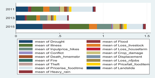
The livelihoods of rural households in Ethiopia are often precarious due to exposure to shocks. These shocks are covariate and idiosyncratic in nature. Covariate shocks affect all households in the village and possibly those nearby, whereas shocks in which the impacts are limited to the household are idiosyncratic (Pradhan & Mukherjee, 2018). The self-reported shocks experienced by rural households over time are depicted in Figure 2. In general, more than 60% of the pooled sample of households have faced at least one type of shock. The temporal distribution of shocks revealed that drought, heavy rain, illness, food price rises, and input price hikes all sharply increases in frequency from 2011/12 to 2015/16. In contrast, loss of farm or house, reductions in food price, landslide, and loss of non-farm jobs remain less frequent and relatively stable over the specified period. More specifically, food price rises, input price hikes, loss of livestock, illness, crop damage, and landslide registered a slight decline in between 2011/12 and 2013/14, but became more frequent in the subsequent rounds. Covariate shocks were found to be more virulent than idiosyncratic ones.

Figure 2. Self-reported shocks.

4.2. Spatiotemporal profile of structural and stochastic poverty

Table 2 exhibits the changes (increases or decreases) in constituent groups over time: it separates out the changes for the first 2011–12 to 2013–14 (column A) and the second period 2013–2014 to 2015–2016 (column B) as well as presenting the overall change from 2011/2012 to 2015/16 (column C). The proportion of households in structural poverty increased over the whole period (by 2.1%) but had in the first period fallen very slightly (0.3%). However, stochastic poverty increased slightly (0.3%) over the whole period, having initially declined (by 0.8%) and then increased (by 1.1%). On the other hand, the stochastically non-poor grew overall (by 3.4%), rising across both periods but more so in the second (Column B, 2.4%). Likewise, those households that were structurally non-poor held steady growth in the first period (0.1%) then declined: this group saw the most change overall as it declined by 5.8% (Column C).

Table 2. Spatial distributions

	Tigray	Amhara	Oromia	SNNP	Others	Total
Structural poor	106(8.05)	373(28.3)	170(12.95)	461(34.9)	208(15.8)	1,318(18.6)
Stochastic poor	154(8.6)	555(31.3)	266(14.9)	541(3.4)	263(14.8)	1,779(25.1)
Stochastic non-poor	215(13.7)	297(18.8)	359(22.8)	361(22.8)	347(21.9)	1,579(22.2)
Structural non-poor	326(13.5)	461(19.0)	545(22.5)	488(2.1)	604(24.9)	2,424(34.1)
Total	801(11.3)	1,686(23.7)	1,340(18.8)	1,851(26.1)	1,422(20.03)	7,100 (100)

The distribution of structural and stochastic poverty among regions shows stark disparities over this period. Table 3 presents the spatial distributions of the incidence of structural and stochastic poverty in Ethiopia. Structural and stochastic poverty appear to be concentrated in SNNP, Amhara, and Others. The higher distribution of poverty in these regions is generally attributed to households experiencing a higher frequency of recurrent and concurrent shocks and having fewer coping resources, productive assets, worse infrastructure, and inadequate social services as compared to Tigray and Oromia (Planning and Development Commission, 2018). Exposure to risks is more pronounced in SNNP and others because these regions have the highest proportion of pastoral areas in Ethiopia. Not only does this greater exposure to shocks markedly erode livelihood potentials through the deterioration of productive assets in the long run in these regions, but pastoral areas also have less diversified income sources and limited commercial orientation (Benti et al., 2022) to turn to when primary sources falter. Tigray and Oromia have the lowest proportions of structural and stochastic poverty, and the highest proportions of non-poor households. Tigray region is the most urbanized region and has relatively better access to basic services, social safety net, asset, and adaptive capacity corroborating than other regions (Haile et al., 2021). Oromia region is located close to Addis Ababa, and households in this region are able to earn better incomes through low-skilled laboring in the capital city because wages are normally higher than in rural areas (Ketema & Diriba, 2021).

Table 3. Transition matrices

Structural
2015/16
2011/12		Poor	Non-poor
	Poor	Twice poor (6.83)	Upward mobile (10.63)
	Non-poor	Downward mobile (18.04)	Twice non-poor (64.49)
	Total	(24.87)	(75.12)
Stochastic
2011/12		Poor	Non-poor
	Poor	Twice poor (4.18)	Upward mobile (13.28)
	Non-poor	Downward mobile (15.16)	Twice non-poor (67.37)
	Total	(19.34)	(80.65)

4.3. Structural and stochastic poverty dynamics

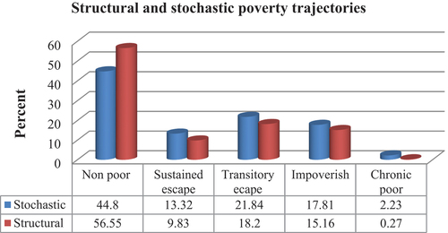
Figure 3 depicts segment of the population poverty trajectories and the share per trajectory. A common finding in this study is that transitory escape and impoverishment comprise a rather large share of the poverty trajectories. Nearly 40% (structurally) and 33.26% (stochastically) of households are either impoverished or transitory escapers. This implies that many households churn around the poverty line. Our analysis confirms, as other researchers have observed (Diwakar & Shepherd, 2018), that the rates at which rural households experienced descents or impoverishment greatly outweigh the rates with which they are able to make sustained escapes. This indicates that structurally positioned and stochastically positioned households are transitioning into and out of poverty at high rates. Indeed, a larger share of stochastically non-poor remains out of poverty over time in the face of shocks as compared to structurally non-poor. Strikingly, only 2.23% of structurally poor and 0.27% of stochastically poor remained chronically poor. This accentuates the inherent stochasticity of income measures of welfare. People are better off one time than another without any significant change in their stock of productive assets.

Figure 3. Poverty trajectories.

Fluidity is an essential characteristic of poverty. We can deduce the net change in the stock of poverty between successive measurements, but we can say nothing from these data about how many people actually escaped poverty and how many others fell into poverty. Experiencing ascents is insufficient to reduce poverty unless descents are simultaneously addressed. Table 4 presents the findings of the poverty transition matrices, reflecting the proportion of households in each welfare class (represented by the row of the table) and that were observed in the next year’s welfare class (the column of the table). It shows the flow of ascents and descents, and the certain degree of persistence between 2011/12 and 2015/16. Out of the total poor in 2011/12, 6.83% and 4.18% remained structural and stochastic poor in 2015/16. However, 13.28% and 10.63% of stochastic and structural poor households experienced upward mobility. These higher stochastic transitions reflect the wider transition in Ethiopia from farm to non-farm livelihoods (World Bank, 2020). This indicates that upward movements were widely stochastic. Of the downward mobiles, 15.16% and 18.04% were due to stochastic and structural transitions. Of the downward mobiles, 15.16% and 18.04% were due to stochastic and structural transitions. Among the twice poor in 2011/12 and 2015/16, the structural and stochastic poor constitute 6.83% and 4.18%. It results on the upheaval in a net growth of structural (2.1%) and stochastic (0.3%) poverty in Ethiopia (see Table 2).

Table 4. Descriptive statistics

	Structurally				test statistics	Stochastically				test statistics
	NP (N = 1454)	UM (N = 289)	DM (N = 352)	P (N = 91)		NP (N = 1250)	UM (N = 380)	DM (N = 386)	P (N = 154)
Attributes and capacities
Age	46.37	48.56	46.06	45.04	3.609	46.79	45.78	47.07	45.34	13.04***
Household size	5.045	5.491	5.569	5.651	7.286***	4.936	5.357	5.599	6.092	1.292
Female-headed (Yes = 1)	0.234	0.215	0.257	0.275	2.112	0.264	0.177	0.217	0.195	15.86***
Education (Literate = 1)	0.343	0.297	0.296	0.247	2.722	0.369	0.263	0.286	0.233	10.28**
Resource base
Income (Ethiopian Birr)	9091	6900	7048	6408	502.3***	8939	8614	6843	7086	538.6***
Land (hectare)	0.396	0.536	0.485	0.386	0.150***	0.381	0.611	0.396	0.437	0.100***
Livestock-owned (TLU)	5.089	3.863	5.126	3.707	90.59***	5.047	4.736	4.539	4.651	54.85***
Oxen for plow (#)	0.947	0.843	0.924	0.715	2.810	0.950	0.868	0.840	1.000	41.81***
Farm plots (#)	8.695	8.982	9.448	9.091	11.52***	8.652	8.006	9.340	9.364	2.660
Skilled non-farm workers (#)	0.889	0.794	0.739	0.772	10.58**	0.809	0.903	0.603	0.597	46.17***
Household activities
Commercialization index	13.71	12.80	7.692	9.549	40.62***	9.956	7.014	12.56	9.505	14.03***
Share of non-farm income (%)	0.297	0.264	0.281	0.264	0.639	0.274	0.258	0.284	0.206	1.995
Wage participation (Yes = 1)	0.115	0.101	0.103	0.064	13.31***	0.108	0.092	0.131	0.103	11.43**
Shocks
Drought shock (Yes = 1)	0.151	0.166	0.203	0.179	9.106**	0.111	0.201	0.191	0.148	21.45***
Production shock (Yes = 1)	0.037	0.122	0.133	0.142	51.71***	0.181	0.235	0.245	0.188	11.63***
Price shock (Yes = 1)	0.047	0.125	0.122	0.131	32.25***	0.194	0.237	0.245	0.258	2.516
Other covariate shocks (#)	0.458	0.612	0.650	0.646	2.180	0.576	0.583	0.721	0.621	20.68***
Other idiosyncratic shocks (#)	0.322	0.315	0.377	0.495	13.46***	0.327	0.357	0.338	0.364	2.591
Others
Credit (Yes = 1)	0.234	0.208	0.298	0.174	8.446***	0.212	0.291	0.234	0.320	12.23***
Distance to the market (Km)	66.85	78.40	74.37	90.04	9.738**	66.61	75.46	76.60	74.49	18.00***
Distance to the town (Km)	40.77	40.27	39.91	46.51	31.84***	40.89	39.55	42.74	38.42	33.70***
Irrigation (Yes = 1)	0.151	0.106	0.098	0.036	314.9***	0.157	0.160	0.135	0.120	106.48***

Notes: NP = non poor, UM= upward mobile, DM = downward mobile, and P = poor.

4.4. Descriptive statistics

Table 5 presents the summary statistics of the variables used in the model, distinguishing the structural and stochastic poor and non-poor households, and moving up and down for the sample. It also unravels how far these different groups are exposed to shocks and suggests how and why they experience the trajectories that they have had. In many of the variables, there were significant differences among the welfare transition categories.

Table 5. Multinomial logit model results

	Structural poor			Stochastic poor			Stochastic non-poor
	Coef.	Std.Err	dy/dx	Coef.	Std.Err	dy/dx	Coef.	Std.Err	dy/dx
Structural non-poor	Base outcome
Resilience capacity	−48.24***	2.307	−4.524***	−40.46***	1.977	−5.323***	−5.52***	1.493	3.236***
Age	−0.007	0.015	0.0002	0.002	0.014	0.002	−0.022*	0.013	−0.004*
Age squared	0.0001	0.0001	0.0001	−0.0001	0.0001	−0.0001	0.0001**	0.0001	0.0001**
Household size	0.426***	0.020	0.039***	0.397***	0.018	0.055***	0.039**	0.018	−0.033***
Female headship	0.367***	0.094	0.034***	−0.040	0.088	−0.045***	0.397***	0.078	0.064***
Number of farm plots	0.553***	0.090	0.014	1.180***	0.079	0.191***	0.236***	0.075	−0.053***
Education	−0.044	0.119	0.002***	−0.344***	0.116	−0.063***	0.102	0.100	0.041***
Extension	−0.245***	0.083	−0.024***	0.035	0.074	0.030**	−0.241***	0.072	−0.038***
Share of non-farm income	−7.306***	1.256	−0.647***	−5.308***	1.097	−0.546***	−2.655***	0.997	0.101
Commercialization	−0.028***	0.003	−0.002***	−0.035***	0.003	−0.005***	−0.006***	0.002	0.002***
Access to irrigation	−0.276***	0.078	−0.027***	−0.138**	0.060	−0.009	−0.104*	0.057	−0.001
Wage labor participation	0.004	0.003	0.001*	0.005**	0.002	0.001***	−0.007***	0.002	−0.002***
Distance to the town	0.006***	0.001	0.001***	0.005***	0.001	0.001***	0.001**	0.001	0.0001**
NDVI	−0.007***	0.001	−0.001***	−0.005***	0.001	−0.001***	0.0001	0.001	0.001***
Covariate shocks	0.931**	0.449	0.062	0.528	0.410	0.002	1.012***	0.336	0.122**
Idiosyncratic shock	0.466	0.676	0.048	0.503	0.587	0.086	−0.177	0.482	−0.081
Production shock	2.397**	1.064	0.285	−0.458	0.888	−0.239***	1.827**	0.780	0.218
Market shock	2.036*	1.147	0.483**	−1.179	0.938	−0.220***	−0.824	0.777	−0.183**
Rainfall variability	0.001	0.002	0.0002	−0.001	0.002	−0.0001	−0.001	0.002	0.0001
Resilience * production shock	−10.51**	4.264	−1.159**	1.435	3.414	1.056*	−6.672**	2.952	−0.934*
Resilience * market shock	−9.37**	4.605	−1.499***	4.500	3.593	0.981*	3.212	2.906	0.683
Resilience * rainfall variability	−0.004	0.010	−0.001	0.004	0.008	0.001	0.002	0.007	0.0001
Resilience * covariate shocks	−3.420*	1.771	−0.218	−2.370	1.569	−0.092	−3.601***	1.265	−0.400*
Resilience * idiosyncratic shocks	−1.672	2.662	0.169	−1.902	2.244	−0.326	0.626	1.782	0.295
Constants	11.35***	0.720	0.001*	9.07***	0.634	0.001***	1.975***	0.537	−0.002***
Observations	7100

LR chi2 (72) = 2490.9, prob> chi2 = 0.0000, pseudo R2 = 0.1289, and log likelihood = −8415.3.

Notes: *, **, *** 1%, 5%, and 10% respectively.

The structurally and stochastically non-poor comprise 64.49% and 67.37% of the sample population. Overall, the non-poor segment of our sample appears to be less exposed to shocks. The structural non-poor encountered only 0.047% of price shocks, while the stochastic non-poor are affected by 0.037% of production shocks. Rural households became non-poor in both cases because they are less prone to idiosyncratic and other covariate shocks. Other notable features of stochastic non-poor households include better market orientation, literacy, and proximity to the market and towns. This holds in many cases in Ethiopia, particularly in rural areas located close to major towns. They often participate in wage labor and earn more income. Likewise, the structural non-poor are also more likely to participate in wage labor and the non-farm economy. They also possessed more nuanced access to irrigation. This is consistent with the findings of Radeny et al. (2012) in rural Kenya.

A smaller proportion of households moving up structurally and stochastically experienced an improvement in their asset positions. Their attributes (household composition, including household size rationalized with more earning members relative to dependents and age expressed in terms of knowledge of farming and experience) and capacities (such as literacy of the head) are more likely to enhance upward mobility than other poverty trajectories. The lowest proportions of female households are more upwardly mobile and the non-poor compared to downward mobiles and the poor. Besides, the structural upward mobiles are generally endowed with better land resources, while their stochastic counterparts have better access to irrigation. The other prominent features of these households are that stochastic trajectories have a larger number of better-skilled farm workers per household than the non-poor. Generally, the upwardly mobile households are less stricken by a number of idiosyncratic and covariate shocks. Likewise, shocks related to climate, price, and production are less pronounced in this welfare transition category compared to the non-poor.

It is the second largest welfare group, accounting for 18.04% and 15.16% of households, in the sample population. The structural and stochastic downward mobiles are distinct, with the lowest financial and physical capital, commercialization, literacy, and economically non-active members next to their poor counterparts. More than a quarter (28.1% and 28.4%) of households in this group unexpectedly generates income from non-farm economic activities. Exposure to a series of shocks is associated with downward mobiles. This category experienced shocks related to drought and numbers of covariates more than other welfare transitions.

The twice poor are the smallest group with 6.83% and 4.18% characterized by having an inadequate endowment of resource bases. The size of cultivated land is very small for structurally poor compared to other welfare transition categories. In contrast, the stochastic poor possessed better land resources than the downwardly mobile and the non-poor. Wealth represented by livestock indicates similar trends (3.707 and 4.651 TLUs). The average incomes, respectively, are 6408 ETB and 7086 ETB. In addition, these households are less connected to towns and markets that are meaningful hubs to engage in economic transactions. As a result, they are less likely to engage in wage labor and the non-farm economic activities. Other notable features of this group of households include inadequate access to irrigation and poor market orientation. Exposure to shocks is also an important caveat to their welfare. Drought, production, and marketing shocks and numbers of other covariate and idiosyncratic shocks deter the ability to escape structural and stochastic poverty. Indeed, other research has found that shocks accompanied by weak conversion factors exacerbate the perseverance of poverty (Diwakar & Shepherd, 2018).

4.5. Econometric results

4.5.1. Effects of resilience and shocks on structural and stochastic poverty

Table 6 presents the estimated results of the multinomial logit model and shows the marginal effects of resilience and shocks on structural and stochastic poverty. It reports on the effects of different covariates affecting the risks of being stochastically non-poor, stochastically poor, and structurally poor (as compared to the base, being structurally non-poor). The Hausman Independence of Irrelevant Alternatives test revealed that the assumption is not violated, and thus the use of multinomial logit is appropriate. The covariates are jointly significant at p < 0.01, and the pseudo-R² value associated with the model is 0.128, indicating that the model’s fitness is satisfactory.

Table 6. Cox proportional hazard model estimates

	Structural entry		Structural exit		Stochastic entry		Stochastic exit
	Coef.	Std. Err.	Coef.	Std. Err.	Coef.	Std. Err.	Coef.	Std. Err.
Resilience capacity	−4.789***	0.625	2.477***	0.446	−3.294***	0.577	2.081***	0.487
Lag resilience capacity	−2.479***	0.587	1.622***	0.396	−1.860***	0.551	1.523***	0.414
Rainfall variability	0.006***	0.002	−0.005*	0.003	0.007***	0.002	−0.008***	0.003
Drought	0.000**	0.000	0.000	0.000	0.000**	0.000	0.000	0.000
Flooding	0.064***	0.019	−0.011	0.018	0.036*	0.018	−0.090**	0.044
Conflict	0.001	0.001	−0.085**	0.035	0.115***	0.036	0.013	0.029
Price shock	−0.075	0.063	0.017	0.028	−0.011	0.042	−0.184***	0.012
Idiosyncratic shocks	0.028	0.029	−0.069**	0.034	0.030	0.028	−0.340***	0.038
NDVI	−0.672***	0.055	−0.048	0.042	−0.565***	0.051	0.010	0.018
Age of household head	0.000	0.001	0.000	0.001	0.000	0.001	0.001	0.001
Household size	0.015	0.013	−0.180***	0.011	0.000	0.012	0.009***	0.001
Female household head	0.003**	0.001	−0.001	0.001	0.004***	0.001	−0.133***	0.036
Education	−0.095**	0.044	0.009***	0.001	0.000	0.001	0.045	0.058
Share of non-farm income	−0.138***	0.037	0.119**	0.053	0.020	0.057	−0.001	0.001
Irrigation	−0.123***	0.039	0.093**	0.041	−0.076**	0.035	0.032	0.043
Observations	7,082		7,082		7,082		7,082

Notes: *, **, *** 1%, 5%, and 10% respectively.

4.5.1.1. Structural poor

The findings validated the fact that structurally poor are more sensitive to covariate, market, and production shocks than the structurally non-poor ones. The marginal effects are also significant and highest for market shocks (0.483 at 5%), followed by production (0.285) and covariate (0.062) shocks. The plausible explanation is that shocks ultimately cause losses in incomes, crops, and livestock, a decline in consumption, social instability, and eventually obliterating households’ asset gains (Borgomeo et al., 2018; Dimitrova, 2021; Gebrechorkos et al., 2020).

Demographics, number of farm plots, and distance to towns matter most critically in structural poverty compared to the base. Female headships are more likely to remain structurally poor by virtue of less empowerment and access to assets in Ethiopia. The size of the household and number of farm plots are positive and significant due to dependence and the diminishing return to scale. The employment effects in the surrounding hinterlands are greater. Besides, households distant from towns experienced structural poverty relative to the base. Poverty declines faster when people live close to towns or leave agriculture for towns since the links between farms and households can be better maintained. The marginal effects are significant and highest for household size (0.039), female headship (0.034), number of farm plots (0.014), and distance to the town (0.001).

In contrast, resilience had a savior role against structural poverty compared to the base. A unit addition of resilience score cutback structural poverty by a factor of 3.239. The interaction terms between resilience and price, production, and idiosyncratic shocks reveal that household resilience eliminates structural poverty compared to the base as shocks escalate. The marginal effects of these variables are also found to be significant and highest for covariate shocks (0.218), followed by market (1.499) and production (0.1159) shocks.

Smallholder farming’s integral part of protecting structural poverty is required to be tapped via irrigation, commercialization, and extension. The marginal effects of these variables are also found to be significant and highest for irrigation (0.027), followed by extension (0.024) and commercialization (0.002). Nevertheless, the sector is fraught with shocks and remains less remunerative for upward structural mobility. Therefore, enhancing non-farm activities is imperative. Equally important, better NDVI reduces structural poverty compared to the base. The marginal effect shows that the likelihood of being structurally poor declines by a factor of 0.001as NDVI increases by a unit.

4.5.1.2. Stochastic poor

Poor households are likely to have significant deficiencies in their resilience capacities as compared to nonpoor households. This is particularly the case for those households who are stochastically poor. The findings also revealed a sturdy positive impact of resilience on the stochastic poor relative to the structural non-poor. It is seen that the risk of being stochastic poor declines by a factor of 5.32 when resilience grows by a unit.³ This implies that reducing stochastic poverty would do well when focusing on resilience as a conduit mechanism or enabling factors that can enhance the resilience of smallholders and their farming systems. According to Haile et al. (2021), all pillars contribute to developing the resilience of farming households. Therefore, better asset endowments, adaptive capacity, social safety nets, and access to social services better protect households against stochastic poverty, ceteris paribus.

The education and skill at the household level are captured by the literacy of the household head. The results show that households headed by more educated ones are less likely to be stochastic poor compared to the structurally poor. The possible explanation is that literacy is associated with the ability to open up potential pathways for diversifying non-farm activities, obtain jobs in the formal sector, and increasing income and knowledge of productive asset building and their return (Dutta & Kumar, 2015). The share of non-farm economy is also associated with reduced vulnerability. The results also revealed that a better share of the non-farm income has a negative and significant correlation with stochastic poverty relative to the base. The risk of being stochastic poor is 0.546 times lower than that of structurally non-poor with a unit growth in the share of non-farm income. Because farming has not been remunerative enough (Dagunga et al., 2020), a better share of the non-farm economy signifies a strong rural economy because of the greater share of casual laborers’ access to formal jobs and enhanced productive asset base.

Likewise, the study finds that access to irrigation and commercialization has a strong positive impact on reducing stochastic poverty compared to the base outcome. Their negative and significant coefficients indicate their vital role in tapping the farming potential, leading to higher yields and income, reduced risk of crop failure, and higher farm and non-farm employment (Gebregziabher et al., 2009). Irrigation also enables smallholders to switch from subsistence to market-oriented production. Besides, households located far away from the market centers are more likely to be stochastically poor than structurally poor, perhaps, due to limited integration to the market. According to Hanjra et al. (2009), the complementarities of irrigation and markets with education are also crucial in generating more earnings and reducing deprivations. Their marginal effects are significant and highest for education (0.063), followed by irrigation (0.009) and distance to the town (0.001). The marginal effects also revealed that growth in the index of commercialization by a unit reduces stochastic poor by a factor of 0.001 compared to structurally non-poor. This finding is in line with Cazzuffi et al. (Cazzuffi et al., 2020). Furthermore, our findings for the NDVI,⁴ which measures sensitivity to drought, indicate that living in an area that is less sensitive to drought is vital in determining stochastic poverty relative to the base. It is shown that a unit less of sensitivity to drought as measured by the NDVI decreases the risk of being stochastically poor by a factor of 0.001.

It is shown that the risk of being stochastic poor compared to structural non-poor is higher for households with larger household sizes and number of farm plots. The marginal effect of these variables is higher for the number of farm plots (0.191) than for household size (0.055). Number of farm plots is a proxy for land fragmentation (Postek et al., 2019) and could influence stochastic poverty either way as witnessed in previous empirical works. The arguments on the impacts of land fragmentation may depend on the demand side and supply side factors. The arguments on the demand side factors assert that farmers voluntarily choose beneficial level of land fragmentation as it helps them avoid labour shortages, spreads risks of crop failure, allows crop rotation and fallow, and promotes use of more fertilizers. The latter merely treats land fragmentation as an exogenous imposition on smallholders, hence detrimental to productivity as it hinders mechanization of agriculture and creates inefficiency in the allocation of labour and capital. In this study, the demand side factor outweighs.

Wage income is among the diversified strategies pursued to escape poverty but is also important for those households which are better-off. Contrary to the earlier proposition, the likelihood of being stochastically poor compared to structurally non-poor is higher for households who participated in wage labor. However, interpreting the implications of larger shares of non-farm income is complex since a greater share of non-farm activities is sometimes symptomatic of a weak rural economy in which rural youths are abandoning agriculture. Moreover, as Bezu and Holden (2014) noted, having a larger share of casual labourers in the absence of access to formal jobs can erode the asset base of households.

4.5.1.3. Stochastic non-poor

Table 6 provides variables determining the risk of stochastic poor compared to structural non-poor. Multiple linked factors affect the stochastic non-poor households relative to the base outcomes. The finding verified the malign effects of exposure to different types of shock. Covariate and production shocks adversely and significantly affect the stochastic non-poor compared to the structural non-poor. The marginal effect of these variables is higher for production shocks (0.218) than number of covariate shocks (0.122). Other researchers also conclude that these shocks aggravate stochastic downward mobility through reduced crop yields, incomes, and consumption and loss of assets (Boansi et al., 2021; Demeke et al., 2011; Ngoma et al., 2019). When prolonged and multiple, shocks result in a downward spiral of asset loss and impoverishment that ultimately limits years of development gains and efforts to interrupt the stochastic transition into poverty (Campos et al., 2014).

Of demographic features, some have a significant effect relying on experience and the relative strength of size economies against the diminishing return. The positive impact of household size elucidates more economically non-active members among the stochastic non-poor. A large household size is often correlated with diminution of resources and worsening impoverishment⁵ (Dutta & Kumar, 2015; Libois & Somville, 2018; Tsehay & Bauer, 2012). Younger households (represented by the age of the head) are associated with lower status of stochastic non-poor, while it would gradually decrease as household heads get older (embodied in the square of age of the head). Moreover, female headship appears to be associated with higher stochastic non-poor compared to the base. It reflects females’ low level of empowerment and entitlement to valuable resources in rural Ethiopia.

Households having a greater number of farm plots (a proxy for land fragmentation) are more likely to be stochastically non-poor compared to the structural non-poor. Land fragmentation is lowering food productivity and simultaneously increasing poverty corroborating the study by Dutta (2021). Likewise, households located distant to towns increase the likelihood of staying stochastic non-poor compared to the base. The marginal effect is highest for farm plots (0.053) followed by distance to towns (0.0001). Proximity to town reduces being stochastic non-poor significantly. Households earn better income as they engage in wage labor in nearby towns and rent out lands (Bezu & Holden, 2014). Therefore, they experienced a stochastic transition out of poverty due to the centrifugal economic spread effect (Diao et al., 2019).

Resilience also has a significant association with the stochastic non-poor. The marginal effect upholds that being stochastic non-poor decreases by a factor of 1.49 when resilience increases by a unit. The interaction terms between resilience and covariate and production shocks are negative and significant. This implies that building resilience protects the stochastic non-poor compared to the base from detrimental impacts of shocks. Resilience serves as a hedge against asset depletion in the presence of shocks since they are more likely to harvest environmental products serving as safety nets (Angelsen & Dokken, 2018).

Improved access to irrigation supplemented with the non-farm economic activities holds the key to stochastic transition out of poverty. In agreement with the above proposition, irrigation and the share of non-farm income significantly reduce the likelihood of staying stochastic non-poor compared to the structural poor by factors of 0.001 and 0.101. Irrigators can maximize yields and crop revenue, diversify sources of income, and accumulate assets which help households mitigate shocks (Burney & Naylor, 2012; Gebregziabher et al., 2009; Huang et al., 2006; Tefera et al., 2020). Households engaging in non-farm economic activities augment farm income to purchase farm inputs and incentive goods. Consequently, it induces a positive spillover effect on farm production, and thus provides an important risk management tool (Danso-Abbeam et al., 2020).

4.5.2. Effects of resilience and shocks on structural and stochastic poverty transitions

The parallel poverty flow configurations are asymmetric in terms of reasons (Krishna, 2007). Table 7 depicts that climate-induced shocks such as rainfall variability and drought exacerbate structural and stochastic poverty entry corroborating other studies (Letta et al., 2018; Maganga et al., 2021; Ngoma et al., 2019; Wossen & Berger, 2015). Floods can also heighten structural and stochastic poverty descents consistent with Kawasaki et al. (2020). Shocks aggravate poverty through decline in asset values, crop production, labor market participation, consumption, and income. Protracted shocks appear to have lasting impacts on human capital, mental health, and cognitive potential (Alem & Tato, 2022; Dercon & Porter, 2014). Moreover, conflict (0.115 at 10%) is highly prevalent as a factor contributing to stochastic entry because it destabilizes regions (Akresh et al., 2012; Hirvonen et al., 2020; Weldeegzie, 2017).

Table 7. Dimensions and indicators used to estimate resilience

Dimensions	Indicators	References
Access to basic services	Access to clean water Access to improved toilet Access to electricity	Exogenous responses provided by the public play a key role in determining the risk exposure of households.
Assets	Land Tropical livestock unit Number of rooms	Assets are part of household wealth, and their availability serves as an important risk coping mechanism. They enhance the resilience capacity of the household to be free from poverty even in the face of shocks and stresses.
Adaptive capacity	Numbers of income sources Subsistence households Food ratio	Households’ capacity to cope with and adapt to certain shocks, so enables households to keep performing their key functions.
Social safety nets	Participation in PSNP Remittances	They comprise formal and informal access to public and private, cash or in-kind transfers to households from different sources that make up a substantial portion of poor households’ annual income.

Female headship is significant at 5% and 10%, respectively, for both structural and stochastic entries, indicating that these groups experience a high probability of poverty entry consistent with Bayudan-Dacuycuy and Lim (2013). Female-headed households in Ethiopia are meager in asset ownership, consumption, and the ability to cope with shocks.

In contrast, several factors protect poverty entry, both structurally and stochastically. Accordingly, resilience and its lagged value significantly insulate structural and stochastic poverty descents. The higher the extent of resilience, the more significant will be the safety and cargo-net effects. Last year’s resilience is a sentinel of current downward mobility too. Likewise, a household with literate heads significantly protect structural and stochastic poverty descents. Besides, households move out of structural and stochastic poverty on account of access to irrigation because they safeguard plunges by raising crop revenue and enhancing the rate of technology adoption (Zewdie et al., 2019).

Farming’s potency is unlikely to continue as land pressure increases with population growth. The result also reveals that an increase in the share of non-farm income has all-importance in protecting structural poverty entry. Furthermore, NDVI is determined by inhibiting structural and stochastic poverty entries as high natural vegetation exhibited less sensitivity to drought (Tonini et al., 2012; Zhang & Zhang, 2019).

Poor households escape poverty due to multiple sets of reasons. Resilience and its lagged values are essential pathways out of poverty. Besides, literacy, irrigation, and the share of non-farm income play a decisive role in escapes. Well established in the literature, education augments sturdy exit effects in developing countries (Dutta & Kumar, 2015; Ngoma et al., 2019). Better participation in the non-farm economy, in turn, enhances the structural poverty escapes substantiating Dutta (2021). Irrigation is also highly prevalent in contributing to structural poverty exits as it mitigates drought and its effects on crop yields, income, and nutrition. The impact is preeminent with literacy and engagement in the market (Hanjra et al., 2009).

This study concedes rainfall variability, drought, and flooding markedly hinder poverty escapes as they erode productive assets (Hansen et al., 2019). Conflict also aggravates poverty by damaging infrastructure, destroying assets, and breaking the social fabric. The detrimental effects of early-life conflict on the physical and cognitive potentials have also been reported (Martin-Shields & Stojetz, 2018). Furthermore, the results show that price and other idiosyncratic shocks threaten the ability to escape poverty via decline in consumption and asset depletion (Alem & Söderbom, 2012; Davies, 2010).

Household size has an ambiguous role in poverty exit. The finding reveals that households with more dependency burdens obstruct structural poverty exit. However, household size rationalized by the existence of more economically active members enhances stochastic ascents, corroborating Dutta (2021). Besides, female headship is highly prevalent as a factor holding back stochastic poverty ascents.

5. Conclusions

The general story that emerged from the analyses witnesses exquisite structural gains and stochastic loss between the first two rounds and vice versa in the latter half. The reason why structural and stochastic poverty slightly declining is because of the pronounced reconfiguration of the poor via simultaneous ebbs and grows. Specifically, the stochastic poor exhibit more likely sustained escapes, while a colossal portion experiences transitory structural poverty escapes. Besides, the probability of descent and impoverishment outweighs these rising and falling tides.

Regression results unambiguously underscore the detrimental effects of drought, price volatility, production loss, and other idiosyncratic and covariate shocks in exacerbating structural and stochastic poverty. Moreover, female headship, dependency ratio, fragmentation coupled with small farm size, distance to the town, and wage labor participation are setbacks to curbing structural and structural poverty. In contrast, the result concedes the deterring role of resilience against structural and stochastic poverty conundrums. Resilience marks the ability to withstand and recover from shocks and curb structural and stochastic poverty even in the face of shocks. Nevertheless, it is not the sole steadfast remedy. Commercialization, irrigation, extension, good vegetation cover, non-farm income, literacy, and human capital formation are also imperative.

Identifying drivers and interrupters also refines our understanding of the causes of ascent and descent of structural and stochastic poverty. The Cox proportional hazard regression also answers questions of who is most at risk of falling and who has the best prospects of escaping from structural and stochastic poverty. Multiple linked factors propel the asymmetric flows. Accordingly, resilience, irrigation, literacy, good vegetation cover, and non-farm activities constitute the most important reasons for influencing upward mobility and protecting the decline into poverty. The last year’s resilience is a strong predictor of current structural and stochastic poverty. Furthermore, rainfall variability, drought, conflict, input and output price volatility, and other covariates and idiosyncratic shocks came up as household stressors aggravating the falling tides.

Several interventions to mitigate shocks and enhance resilience are needed to fight against structural and stochastic poverty. There remains the potential for smallholder farming to be an integral part of poverty reduction. However, this potential has to be tapped through improving commercialization and investment in irrigation, non-farm economy, roads and marketing networks, and human capital formation. Nevertheless, the sector is fraught and less remunerative. Critical for policy uptake, strengthening symbiotic rural–urban links ensures a balanced mix of infrastructure development that would bolster the non-farm sector, commercialization, human capital, and livelihood diversification. Therefore, rural revitalization is necessary to reduce structural and stochastic poverty. It requires a transformative approach that considers all aspects of making rural areas a good place to live and work for present and future generations.

The empirical result provides much-needed evidence substantiating state-of-the-art policies encouraging poverty reduction. Thus, policies aimed at eradicating structural and stochastic poverty would do well when focusing on enabling factors that can enhance the resilience of smallholders and their farming systems. Enhancing resilience mitigates the adverse effects of shocks on structural and stochastic poverty. Thus, resilience is required to be mainstreamed as part of any pro-poor intervention.

Policymaking to deal with structural and stochastic poverty has to build up a more comprehensive response. Unless we curtail the creation of new poverty, efforts to ascertain poverty escapes will ultimately be futile. It is preeminent to address both groups’ reasons as they function within the country. Thus, targeting with a polycentric approach makes more headway than aggregate responses. Vulnerability to shocks, illiteracy, and stagnated non-farm economic activities form a chain that leads to a cycle of subsistence and enduring structural and stochastic poverty. Breaking the chain at any point on these links can help rescue many from falling into poverty. Irrigation infrastructures, enhancing the rural non-farm economy, and investing in human capital lay a solid foundation to deter poverty reversals.

Disclosure statement

No potential conflict of interest was reported by the author(s).

Additional information

Funding

This manuscript received no financial grant from any funding agency.

Notes on contributors

Dereje Haile

Dereje Haile is an Assistant Professor of Development Studies. Ample experience with a demonstrated history of working in the higher education, he has research interests in the economics of poverty, food and nutrition insecurity, destitution, resilience, climate change, agricultural productivity, technology adoption, conflict and migration, to address questions that are relevant for sustainable development.

Abrham Seyoum

Abrham Seyoum is an Associate Professor of Development Economics at Addis Ababa University. He has been involved in various research projects in the areas of agricultural and development economics, agricultural productivity, commercialization, poverty and vulnerability, resilience, food security, and destitution. He authored and co-authored numerous journal articles.

Alemu Azmeraw

Alemu Azmeraw is an Associate Professor of Sociology and Development Studies at Addis Ababa University. He has extensive research and teaching experience in the areas of rural transformation, sustainable development, qualitative research methodology, climate change, value chain analysis, poverty, food and nutrition security, destitution, and policy analysis.

Notes

1. The two-stage stratified sampling technique was applied taking into account diversities in agro ecological factors for rural areas and major urban towns for the urban survey. In the first stage, the four most populous regions and a combination of the remaining regions as a fifth category were stratified, from which CSA enumeration areas (EAs) were selected with probability proportional to size. The number of EAs covered by the survey begins with 333 in the first round and grown to 433 (290 rural, 43 small town and 100 major urban areas) subsequently. In the second stage, 12 households in each EA were randomly selected. Out of the 3,969 households in first 2011/12, the later waves respectively re-interviewed 3,776 and 3,699 rural households (CSA and World Bank, 2017).

2. It entails a total of 6 dwelling characteristics, 31 household durables, and 4 household means of production. Variables with low standard deviations or an asset that all households own or no one owns that would exhibit no variation between households and would be zero weighted that would carry a low weight from the PCA were excluded.

3. Since the coefficients of each covariates are relative to the reference group (structural non-poor), the standard interpretation of the multinomial logit is that for a unit change in the predictor variable (For example, resilience capacity), the logit of the outcome relative to the referent group is expected to change by its respective parameter estimate given the variables in the model are held constant.

4. Normalized Difference Vegetation Index is a simple index that allows immediate recognition of problems in farm areas. It is used as a proxy for water stress problems (vulnerability to drought) or land productivity or the state of land degradation Zhang and Zhang (2019). Its values range between −1 and 1, and each value corresponds to a different agronomic situation, regardless of the crop. A better NDVI implies strong vegetation cover and responses to environmental change, less vulnerable to drought (Tonini et al., 2012) and have more production, and resilient properties of the landscapes and their constituent. The greening in vegetation in the rain-fed agricultural areas is strongly linked to living in a more productive land which can be attributed to improved productivity.

5. However, it is not necessarily the case in rural Ethiopia that children are an unsustainable economic burden for a household; rather, it is the combination of children with respect to their timing in a household’s life cycle and income generating capacity which influences the downward mobility of the stochastic non-poor.

References

- RM-TWG. (2014). Resilience measurement principles: Toward an agenda for measurement design. Resilience, No. 1; Food Security Information Network Technical Working Series, Issue 1. Food and Agriculture Organization (FAO) and the World Food Programme (WFP).
- Abebaw, S., Betru, T., & Wollie, G. (2020). Prevalence of household food insecurity in Ethiopia during the COVID-19 pandemic: Evidence from panel data. Scientific African, 16(January), e01141. https://doi.org/10.1016/j.sciaf.2022.e01141
- Akresh, R., Lucchetti, L., & Thirumurthy, H. (2012). Wars and child health: Evidence from the Eritrean-Ethiopian conflict. Journal of Development Economics, 99(2), 330–27. https://doi.org/10.1016/j.jdeveco.2012.04.001
- Alem, Y., & Söderbom, M. (2012). Household-level consumption in urban Ethiopia: The effects of a large food price shock. World Development, 40(1), 146–162. https://doi.org/10.1016/j.worlddev.2011.04.020
- Alem, Y., & Tato, G. L. (2022). Shocks and mental health panel data Evidence from South Africa ( No. 22–01; Environment for Development EfD Discussion Paper Series, Issue February).
- Angelsen, A., & Dokken, T. (2018). Climate exposure, vulnerability and environmental reliance: A cross-section analysis of structural and stochastic poverty. Environment and Development Economics, 23(3), 257–278. https://doi.org/10.1017/S1355770X18000013
- Bader, C., Bieri, S., Wiesmann, U., & Heinimann, A. (2016). Differences between monetary and multidimensional poverty in the Lao PDR: Implications for targeting of poverty reduction policies and interventions. Poverty and Public Policy A Global Journal of Social Security, Income, Aid, and Welfare, 8(2), 171–197. https://doi.org/10.1002/pop4.140
- Barrett, C. B. (2005). Rural poverty dynamics: Development Policy implications. Agricultural Economics, 32(s1), 45–60. https://doi.org/10.1111/j.0169-5150.2004.00013.x
- Barrett, C. B., & Constas, M. A. (2014). Toward a theory of resilience for international development applications. Proceedings of the National Academy of Sciences of the United States of America, 111(40), 14625–14630. https://doi.org/10.1073/pnas.1320880111
- Barua, S., & Banerjee, A. (2020). Impact of climatic shocks on household well-being: Evidence from rural Bangladesh. Asia-Pacific Journal of Rural Development, 30(1–2), 89–112. https://doi.org/10.1177/1018529120977246
- Bayudan-Dacuycuy, C., & Lim, J. A. (2013). Family size, household shocks and chronic and transient poverty in the Philippines. Journal of Asian Economics, 29, 101–112. https://doi.org/10.1016/j.asieco.2013.10.001
- Bekele, Y. W. (2018). The political economy of poverty in Ethiopia: Drivers and challenges. African Review, 10(1), 17–39. https://doi.org/10.1080/09744053.2017.1399561
- Béné, C., Cannon, T., Gupte, J., Metha, L., & Tanner, T. (2014). Exploring the potential and limits of the resilience agenda in rapidly urbanizing contexts. IDS Evidence Report, (63). https://opendocs.ids.ac.uk/opendocs/handle/123456789/3621
- Béné, C., Headey, D., Haddad, L., & von Grebmer, K. (2016). Is resilience a useful concept in the context of food security and nutrition programmes? Some conceptual and practical considerations. Food Security, 8(1), 123–138. https://doi.org/10.1007/s12571-015-0526-x
- Benti, D. W., Biru, W. T., & Nd Tessema, W. K. (2022). The effects of commercial orientation on (agro) pastoralists’ household Food Security: Evidence from (agro) pastoral communities of Afar, Northeastern Ethiopia. Sustainability (Switzerland), 14(2). https://doi.org/10.3390/su14020731
- Berkes, F., & Ross, H. (2013). Community resilience: Toward an integrated approach. Society and Natural Resources, 26(April 2013), 5–20. https://doi.org/10.1080/08941920.2012.736605
- Bezu, S., & Holden, S. (2014). Are rural youth in Ethiopia abandoning agriculture? World Development, 64, 259–272. https://doi.org/10.1016/j.worlddev.2014.06.013
- Boansi, D., Owusu, V., Tambo, J. A., Donkor, E., & Asante, B. O. (2021). Rainfall shocks and household welfare: Evidence from Northern Ghana. Agricultural Systems, 194(September), 103267. https://doi.org/10.1016/j.agsy.2021.103267
- Borgomeo, E., Vadheim, B., Woldeyes, F. B., Alamirew, T., Tamru, S., Charles, K. J., Kebede, S., & Walker, O. (2018). The distributional and multi-sectoral impacts of rainfall shocks: Evidence from computable general equilibrium modelling for the awash basin, Ethiopia. Ecological Economics, 146(April 2017), 621–632. https://doi.org/10.1016/j.ecolecon.2017.11.038
- Brück, T., & Workneh Kebede, S. (2013). Dynamics and drivers of consumption and multidimensional poverty: Evidence from rural Ethiopia. IZA Discussion Paper Series, (7364), IZA Discussion Paper. https://doi.org/10.2139/ssrn.2263600
- Burney, J. A., & Naylor, R. L. (2012). Smallholder irrigation as a poverty alleviation tool in sub-Saharan Africa. World Development, 40(1), 110–123. https://doi.org/10.1016/j.worlddev.2011.05.007
- Campos, A. P. O., Villani, C., Davis, B., & Takagi, D. (2014). Ending extreme poverty: Sustaining livelihoods to leave No one behind. The World Bank. http://www.worldbank.org/en/publication/global-monitoring-report/report-card/twin-goals/ending-extreme-poverty
- Carter, M. R., & Barrett, C. B. (2006). The Economics of poverty traps and persistent poverty: An asset-based approach. The Journal of Development Studies, 42(2), 178–199. https://doi.org/10.1080/00220380500405261
- Carter, M. R., & Lybbert, T. J. (2012). Consumption versus asset smoothing: Testing the implications of poverty trap theory in Burkina Faso. Journal of Development Economics, 99(2), 255–264. https://doi.org/10.1016/j.jdeveco.2012.02.003
- Carter, M. R., & May, J. (1999). Poverty, livelihood and class in rural South Africa. World Development, 27(1), 1–20. https://doi.org/10.1016/S0305-750X(98)00129-6
- Cazzuffi, C., Mckay, A., & Perge, E. (2020). The impact of agricultural commercialisation on household welfare in rural Vietnam. Food Policy, 94(November), 101811. https://doi.org/10.1016/j.foodpol.2019.101811
- CEPHEUS. (2020). Macroeconomic impacts of the corona virus: A preliminary assessment for Ethiopia. Macro Research Ethiopia.
- Cox, D. R. (1972). Regression models and Life-Tables. Journal of the Royal Statistical Society 1, 34(2), 187–220. https://doi.org/10.1111/j.2517-6161.1972.tb00899.x
- CSA and World Bank. (2017). Ethiopia socioeconomic survey (ESS) wave three (2015/2016) basic information document. Central Statistical Agency & Living Standards Measurement Study (LSMS). World Bank, Addis Ababa. https://doi.org/10.48529/ampf-7988
- Dagunga, G., Ayamga, M. A., & Danso-Abbeam, G. (2020). To what extent should farm households diversify? Implications on multidimensional poverty in Ghana. World Development Perspectives, 20(September), 100264. https://doi.org/10.1016/j.wdp.2020.100264
- Danso-Abbeam, G., Dagunga, G., & Ehiakpor, D. S. (2020). Rural non-farm income diversification: Implications on smallholder farmers’ welfare and agricultural technology adoption in Ghana. Heliyon, 6(11), e05393. https://doi.org/10.1016/j.heliyon.2020.e05393
- Das, P., Paria, B., & Firdaush, S. (2021). Juxtaposing consumption poverty and multidimensional poverty: A study in Indian context. Social Indicators Research, 153(2), 469–501. Springer Netherland. https://doi.org/10.1007/s11205-020-02519-0
- Davies, S. (2010). Do shocks have a persistent impact on consumption? The case of rural Malawi. Progress in Development Studies, 10(1), 75–79. https://doi.org/10.1177/146499340901000105
- Davies, M., Béné, C., Arnall, A., Tanner, T., Newsham, A., & Coirolo, C. (2013). Promoting resilient livelihoods through adaptive social protection: Lessons from 124 programmes in South Asia. Development Policy Review, 31(1), 27–58. https://doi.org/10.1111/j.1467-7679.2013.00600.x
- Demeke, A. B., Keil, A., & Zeller, M. (2011). Using panel data to estimate the effect of rainfall shocks on smallholders food security and vulnerability in rural Ethiopia. Climatic Change, 108(1), 185–206. https://doi.org/10.1007/s10584-010-9994-3
- Dercon, S., & Porter, C. (2014). Live aid revisited: Long-term impacts of the 1984 Ethiopian famine on children. Journal of the European Economic Association, 12(4), 927–948. https://doi.org/10.1111/jeea.12088
- Diao, X., Magalhaes, E., & Silver, J. (2019). Cities and rural transformation: A spatial analysis of rural livelihoods in Ghana. World Development, 121, 141–157. https://doi.org/10.1016/j.worlddev.2019.05.001
- Dimitrova, A. (2021). Seasonal droughts and the risk of childhood undernutrition in Ethiopia. World Development, 141, 105417. https://doi.org/10.1016/j.worlddev.2021.105417
- Diwakar, V., & Shepherd, A. (2018). Sustaining escapes from poverty (No. (539); Overseas Development Institute (ODI) Working Paper, Issue October).
- Dutta, S. (2021). Structural and stochastic transitions of poverty using household panel data in India. Poverty & Public Policy, 13(1), 8–31. https://doi.org/10.1002/pop4.299
- Dutta, S., & Kumar, L. (2015). Is poverty stochastic or structural in nature? Evidence from rural India. Social Indicators Research, 128(3), 957–979. https://doi.org/10.1007/s11205-015-1064-9
- Dutta, S., & Kumar, L. (2016). Is poverty stochastic or structural in nature? Evidence from rural India. Social Indicators Research, 128(3), 957–979. https://doi.org/10.1007/s11205-015-1064-9
- Folke, C. (2006). Resilience: The emergence of a perspective for social-ecological systems analyses. Global Environmental Change, 16(3), 253–267. https://doi.org/10.1016/j.gloenvcha.2006.04.002
- Foster, J., Greer, J., & Thorbecke, E. (1984). A class of decomposable poverty measures. Econometrica, 52(3), 761. https://doi.org/10.2307/1913475
- Gebrechorkos, S. H., Hülsmann, S., & Bernhofer, C. (2020). Analysis of climate variability and droughts in East Africa using high- resolution climate data products. Global and Planetary Change, 186(January), 103130. https://doi.org/10.1016/j.gloplacha.2020.103130
- Gebregziabher, G., Namara, R. E., & Holden, S. (2009). Poverty reduction with irrigation investment: An empirical case study from Tigray, Ethiopia. Agricultural Water Management, 96(12), 1837–1843. https://doi.org/10.1016/j.agwat.2009.08.004
- Gebremariam, G., & Nd Tesfaye, W. (2018). The heterogeneous effect of shocks on Agricultural innovations adoption: Microeconometric Evidence from rural Ethiopia. Food Policy, 74(April 2016), 154–161. https://doi.org/10.1016/j.foodpol.2017.12.010
- Gorst-Rasmussen, A. (2012). Tt: Treelet transform with Stata. The Stata Journal, 12(1), 130–146. https://doi.org/10.1177/1536867X1201200108
- Greene, W. H. (2018). Econometric analysis (8th ed.). Pearson Education, Inc.
- Habtewold, T. M. (2021). Impacts of COVID-19 on Food Security, employment and education: An empirical assessment during the early phase of the pandemic. Clinical Nutrition Open Science, 38, 59–72. https://doi.org/10.1016/j.nutos.2021.06.002
- Haile, D., Seyoum, A., & Azmeraw, A. (2021). Does building the resilience of rural households reduce multidimensional poverty? Analysis of panel data in Ethiopia. Scientific African, 12, e00788. https://doi.org/10.1016/j.sciaf.2021.e00788
- Hanjra, M. A., Ferede, T., & Gutta, D. G. (2009). Pathways to breaking the poverty trap in Ethiopia: Investments in agricultural water, education, and markets. Agricultural Water Management, 96(11), 1596–1604. https://doi.org/10.1016/j.agwat.2009.06.008
- Hansen, J., Hellin, J., Rosenstock, T., Fisher, E., Cairns, J., Stirling, C., Lamanna, C., van Etten, J., Rose, A., & Campbell, B. (2019). Climate risk Management and rural poverty reduction. Agricultural Systems, 172(January 2018), 28–46. https://doi.org/10.1016/j.agsy.2018.01.019
- Hill, R. V., & Porter, C. (2017). Vulnerability to drought and food price shocks: Evidence from Ethiopia. World Development, 96, 65–77. https://doi.org/10.1016/j.worlddev.2017.02.025
- Hirvonen, K., Sohnesen, T. P., & Bundervoet, T. (2020). Impact of Ethiopia’s 2015 drought on child undernutrition. World Development, 131, 104964. https://doi.org/10.1016/j.worlddev.2020.104964
- Holling, C. S. (1973). Resilience and stability of ecological systems. Annual Review of Ecology and Systematics, 4(1), 1–23. https://doi.org/10.1146/annurev.es.04.110173.000245
- Huang, Q., Rozelle, S., Lohmar, B., Huang, J., & Wang, J. (2006). Irrigation, Agricultural performance and poverty reduction in China. Food Policy, 31(1), 30–52. https://doi.org/10.1016/j.foodpol.2005.06.004
- Hulme, D., & Shepherd, A. (2003). Conceptualizing chronic poverty. World Development, 31(3), 403–423. https://doi.org/10.1016/S0305-750X(02)00222-X
- IFRC, and RCS. (2016). Resilience: Saving lives Today, investing for tomorrow. World Disaster Report 2016. International Federation of Red Cross and Red Crescent Societies.
- Kawasaki, A., Kawamura, G., & Zin, W. W. (2020). A local level relationship between floods and poverty: A case in Myanmar. International Journal of Disaster Risk Reduction, 42, 101348. https://doi.org/10.1016/j.ijdrr.2019.101348
- Ketema, M., & Diriba, G. (2021). The state of Ethiopian economy 2020/21: Population dynamics and economic Development. In M. Ketema & G. Diriba (Eds.), The state of Ethiopia economy 2020/21. Ethiopian Economics Association (EEA). Issue February. https://doi.org/10.3934/dcdsb.2021178.
- Krishna, A. (2007). For reducing poverty faster: Target reasons before people. World Development, 35(11), 1947–1960. https://doi.org/10.1016/j.worlddev.2006.12.003
- Krishna, A., & Krishna, A. (2017). The dynamics of poverty. In L. M. Burton (Ed.), The oxford handbook of the social science of poverty (oxford Han (pp. 1–30). Oxford University Press. https://doi.org/10.1093/oxfordhb/9780199914050.013
- Letta, M., Montalbano, P., & Tol, R. S. J. (2018). Temperature shocks, short-term growth and poverty thresholds: Evidence from rural Tanzania. World Development, 112, 13–32. https://doi.org/10.1016/j.worlddev.2018.07.013
- Libois, F., & Somville, V. (2018). Fertility, household size and poverty in Nepal. World Development, 103, 311–322. https://doi.org/10.1016/j.worlddev.2017.11.005
- Maganga, A. M., Chiwaula, L., & Kambewa, P. (2021). Climate induced vulnerability to poverty among Smallholder farmers: Evidence from Malawi. World Development Perspectives, 21(May), 100273. https://doi.org/10.1016/j.wdp.2020.100273
- Mariotti, C., & Diwakar, V. (2016). Ensuring escape from poverty are sustained in rural Ethiopia, leveraging economic opportunities (LEO) report number 36 (Issue August).
- Martin-Shields, C., & Stojetz, W. (2018). Food Security and conflict. Empirical challenges and future opportunities for Research and Policy making on Food Security and conflict. FAO Agricultural Development Economics, 66(1), 18–04. https://doi.org/10.2139/ssrn.2970936
- MoFED. (2012). Ethiopia’s Progress towards eradicating poverty: An interim report on poverty analysis study (2010/11) (Issue March).
- MoFED. (2017). Ethiopia’s Progress towards eradicating poverty: An interim report on 2015/16 poverty analysis study (Issue March).
- Moser, C., Stein, A., Norton, A., & Georgieva, S. (2010). Pro-poor adaptation to climate change in urban centers: Case Studies of vulnerability and resilience in Kenya and Nicaragua. Report No 54947-GLB.
- Ngoma, H., Mulenga, B. P., & Banda, A. (2019). Poverty and weather shocks: A Panel data analysis of structural and stochastic poverty in Zambia ( No. 150; IAPRI Wprking Paper, Issue November). https://doi.org/10.13140/RG.2.2.14838.55363
- Ngoma, H., Mulenga, B. P., Snyder, J., Banda, A., & Chapoto, A. (2019). Poverty and weather shocks: A panel data analysis of structural and stochastic poverty in Zambia. In Feed the Future Innovation Lab for Food Security Policy ( No. 154; Research Paper Series, Issue November).
- OPHI Issue July . (2019). “Ethiopia country briefing”, multidimensional poverty index data Bank. Oxford Poverty and Human Development Initiative (OPHI), Oxford, University of Oxford.
- Phadera, L., Michelson, H., Winter-Nelson, A., & Goldsmith, P. (2019). Do asset transfers build household resilience? Journal of Development Economics, 138(January), 205–227. https://doi.org/10.1016/j.jdeveco.2019.01.003
- Planning and Development Commission. (2018). Poverty and economic growth in Ethiopia (1995/96-2015/16). United Nations Development Program, (December).
- Postek, P., Len, P., & Strek, Z. (2019). The proposed indicator of fragmentation of Agricultural land. Ecological Indicators, 103(March), 581–588. https://doi.org/10.1016/j.ecolind.2019.04.023
- Pradhan, K. C., & Mukherjee, S. (2018). Covariate and idiosyncratic shocks and coping strategies for poor and non-poor rural households in India. Journal of Quantitative Economics, 16(1), 101–127. https://doi.org/10.1007/s40953-017-0073-8
- Radeny, M., van den Berg, M., & Schipper, R. (2012). Rural poverty dynamics in Kenya: Structural declines and stochastic escapes. World Development, 40(8), 1577–1593. https://doi.org/10.1016/j.worlddev.2012.04.027
- Ravallion, M. (2016). The Economics of poverty: History, measurement, and Policy. The Social Science Journal, 55(2). Oxford University Press. https://doi.org/10.1016/j.soscij.2018.03.005.
- Royston, P. (2001). Flexible parametric Alternatives to the Cox model, and more. The Stata Journal, 1(1), 1–28. https://doi.org/10.1177/1536867X0100100101
- Schotte, S. (2019). Structural poverty dynamics in urban South Africa a mixed-methods investigation (No. 100; UNU-WIDER Working Paper, Issue December). https://doi.org/10.35188/UNU-WIDER/2019/736-1
- Shehu, A., & Sidique, S. F. (2020). The effect of shocks on household consumption in rural Nigeria. The Journal of Developing Areas, 49(3), 353–364. https://doi.org/10.1353/jda.2015.0163
- Sou, G. (2019). Sustainable resilience? Disaster recovery and the Marginalization of Sociocultural needs and concerns. Progress in Development Studies, 19(2), 144–159. https://doi.org/10.1177/1464993418824192
- Stifel, D., & Woldehanna, T. (2017). Estimating utility-consistent poverty in Ethiopia, 2000–11. In C. Arndt & F. Tarp (Eds.), Measuring poverty and wellbeing in developing countries (pp. 55–73). Oxford University Press (OUP).
- Swanepoel, C. (2005). Poverty and poverty dynamics in Ethiopia ( No. 3). Stellenbosch Economic Working Papers).
- Tefera, S. A., Tadese, T. B., & Asmare, G. W. (2020). Prevalence of Household Food Insecurity in Ethiopia during the COVID-19 pandemic: Evidence from Panel Data. Scientific African, 16(2022), e01141. https://doi.org/10.1016/j.sciaf.2022.e01141
- Tonini, F., Lasinio, G. J., & Hochmair, H. H. (2012). Mapping return levels of absolute NDVI variations for the assessment of drought risk in Ethiopia. International Journal of Applied Earth Observation and Geoinformation, 18(1), 564–572. https://doi.org/10.1016/j.jag.2012.03.018
- Tran, Q., Alkire, S., & Klasen, S. (2014). Disparities between monetary and multidimensional measurements of poverty. In IARIW 33rd General Conference. Rotterdam, the Netherlands.
- Tsehay, A. S., & Bauer, S. (2012). Poverty and vulnerability dynamics: Empirical Evidence from smallholders in Northern Highlands of Ethiopia. Quarterly Journal of International Agriculture, 51(4), 301–332. https://doi.org/10.22004/ag.econ.155481
- Weldeegzie, S. G. (2017). Growing-up unfortunate: War and human capital in Ethiopia. World Development, 96, 474–489. https://doi.org/10.1016/j.worlddev.2017.03.030
- World Bank. (2015). Ethiopia poverty assessment: Poverty global Practice Africa region. http://hdl.handle.net/10986/21323
- World Bank. (2018). Poverty and shared prosperity: Piecing together poverty puzzle. World Bank.
- World Bank. (2020). Ethiopia poverty assessment: Harnessing continued growth for accelerated poverty reduction. www.worldbank.org
- Wossen, T., & Berger, T. (2015). Climate variability, food security and poverty: Agent-based assessment of policy options for farm households in Northern Ghana. Environmental Science and Policy, 47, 95–107. https://doi.org/10.1016/j.envsci.2014.11.009
- Wulff, J. N. (2015). Interpreting results from the multinomial logit model: Demonstrated by foreign market entry. Organizational Research Methods, 18(2), 300–325. https://doi.org/10.1177/1094428114560024
- Zewdie, M. C., Van Passel, S., Cools, J., Tenessa, D. B., Ayele, Z. A., Tsegaye, E. A., Minale, A. S., & Nyssen, J. (2019). Direct and indirect effect of irrigation water availability on crop revenue in Northwest Ethiopia: A structural equation model. Agricultural Water Management, 220(July), 27–35. https://doi.org/10.1016/j.agwat.2019.04.013
- Zhang, X., & Zhang, B. (2019). The responses of natural vegetation dynamics to drought during the growing season across China. Journal of Hydrology, 574(January), 706–714. https://doi.org/10.1016/j.jhydrol.2019.04.084