European Banking Union structures and dynamics

Abstract

This article begins with an analysis of banking flows in the euro zone, through a complex network, from 2006 to 2020. This analysis allows us to observe the topology of the network through different phases of the business cycle. It is obtained that there is greater fragmentation in the network that increases in three stages, with turning points in crises. In turn, the topological structure is less random and presents more capitalized subnetworks with less risk. As for the nodes of the network, Germany gives up the position of centrality in favor of France. The determinants of the links in the network are analyzed with Machine Learning, obtaining as push and pull bank variables solvency and bank income structure, respectively, and productivity as economic variable.

Keywords:

• complex network
• bank flows
• bank integration
• systemic risk

JEL Classification:

• G01
• G15
• G21
• G28
• C63
• C6

1. Introduction

As a consequence of the 2008 financial crisis and the 2012-euro crisis, two crucial sets of measures were implemented that had an impact on the European banking landscape. Firstly, progress was made in the banking union within the eurozone, leading to the establishment of a resolution and supervision framework by the ECB for the most significant banking groups in the region. This initiative aimed to prevent the fragmentation of the banking market.

Secondly, at the regulatory level, Basel III was developed and subsequently transposed by the EU.¹ This regulation seeks to enhance the strength of European banking groups by improving the quality of regulatory capital. It also establishes leverage ratios, liquidity ratios, and financing ratios that provide financial institutions with greater resilience in the face of crisis events. All these measures have an influence on the behavior of financial institutions, requiring them to adapt to a new regulatory environment.

One of the novelties brought by Basel III was the implementation of macroprudential regulation measures. To this end, countercyclical capital requirements were established to mitigate procyclicality in the banking system, as well as capital surcharges for systemic risk. Therefore, regulatory authorities recognized the need to regulate the latent risk in the system, which may not manifest individually until crisis events occur.

There have been several studies on networks applied to the financial system. Some studies, such as Acemoglu et al. (2015), Amini et al. (2012) and Gai and Kapadia (2010), demonstrate how the financial system exhibits a robust but fragile property, specifying how connectivity influences stability. In particular, connectivity and the size of shocks interact to determine how a financial system can transition abruptly from a state of stability to a state of instability. Other studies focus on the degree of connectivity, specifically Battiston et al. (2012), which show how higher connectivity can lead to increased systemic risk whenever the initial robustness is heterogeneous and many banks are fragile, as an initial set of defaults can trigger a systemic failure.

Other studies, such as Caccioli et al. (2012) and Detering et al. (2019) have focused on exploring the impact on financial system stability based on the diversity of node characteristics. Lenzu and Tedeschi (2012) and Brunetti et al. (2019) have examined the clustering of nodes and the transmission of liquidity according to topological structures. This study employs complex network analysis to examine the European banking system from both a national and dynamic perspective. The research design raises questions about the relationship between banking fragmentation and banking stability in a novel manner.

The literature presents contrasting opinions regarding this relationship. For instance, according to Kose et al. (2009) and Jappelli and Pistaferri (2011), one of the presumed benefits of global financial market integration is its positive impact on stability, as risks are spread globally, and risk-sharing improves consumption smoothing. However, Stiglitz (2010) raises doubts about the benefits of financial integration due to contagion effects during financial crises, and Caballero (2015) discovers a significant impact of financial integration on banking crises. More recent works, such as Devereux and Yu (2020) and Inekwe and Valenzuela (2020), suggest that the impact of a crisis in integrated international financial markets is less severe compared to autarky, although such crises might occur more frequently. Given the European Union’s significant reliance on banks for financing the economy, it becomes imperative to analyze how integration influences financial stability.

In the first part of the study, the focus is on banking networks, considering them highly useful for understanding the formation and concentration of risk in the banking system through the topological formation of the network, as well as its evolution over time. This perspective can constitute an advancement for regulatory and supervisory entities, marking the beginning of a new approach to banking regulation and supervision. This analysis allows observing the interaction of the network’s topological structure with risk, liquidity, and the capitalization of subnetworks. Thus, one of the main contributions of the document is that its approach can constitute a new paradigm for regulatory and supervisory entities by expanding the mandate to detect topological structures that may be more unstable for the financial structure in different phases of the cycle, particularly concerning national banking systems in the Eurozone.

In the second part of the study, the determinants of banking flows in the European Banking Union, which are the links in banking networks, are analyzed. Understanding these flows is crucial for regulators and market participants as it enables effective control of financial stability. The determinants of banking flows also have implications for financial integration and market efficiency within the banking union. Utilizing machine learning techniques, we aim to identify the variables that determine the links within the network. This includes the characteristics of the pipes that transfer banking flows (i.e., the banks), as well as factors related to pressure and economic attractors. To achieve this, two datasets are established: one comprising bank variables and another containing economic variables of the nodes/countries. This allows us to identify the most influential push and pull variables for bank links/flows in both sets of variables. This approach provides insight into the determinants of bank flows, to the best of our knowledge. This is done by placing these flows in gross terms within a complex network, where there are various adaptive interactions within the network, and obtaining the determinants of these flows based on node characteristics using a machine learning methodology.

The research design aims to answer several questions regarding the banking system in the Eurozone, which constitute a novelty in the literature to the best of our knowledge. Among the highlighted questions to be addressed are:

• I. How has the topological structure of the European Banking Union varied over the study period according to different measures, through different phases of the cycle?

• II. How can complex networks be used to measure financial integration and analyze its evolution, identifying different phases?

• III. What characteristics do the subnetworks (center/periphery) within the topological structure exhibit, and how do they interact with different banking variables such as risk and liquidity, among others?

• IV. Which economic and banking push and pull variables are more determinant in the links of complex networks? With this question, we address the importance of the state of channels (banking intermediaries) in banking flows within networks, as well as the characteristics of the nodes in terms of their function as attractors and repellents of banking flows.

The research design begins with a complex network model for the Eurozone banking system, where national banking systems serve as nodes, and the links are formed through consolidated loans based on nationality within that network.

This enables us to observe the behavior of the network and its evolution throughout the study period, spanning from 2006 to 2020. We analyze the subgroups that form within the network during periods of increased fragmentation or the nodes/countries that occupy centrality measures. It will be observed that during the stage of negative interest rates, there is a greater fragmentation of the network, resulting in a decrease in links between nodes, as well as changes in centrality weights in absolute and relative terms among the nodes. These changes can have implications for the transmission of monetary policy, and it is valuable to analyze the topological structure of the network in terms of policy implications. Significantly, our study emphasizes the network-level approach to financial regulation and supervision, alongside an examination of the interplay between banking integration, capitalization, banking risks, and liquidity within the various topological structures of the European banking system.

Furthermore, an analysis of the state of the art is conducted. Section I presents the methodology of complex networks and performs the network analysis for the study period. In Section II, machine learning algorithms are used to identify the push and pull variables, and finally, the conclusions are drawn.

1.1. State of art

This paper links and adds new evidence from two distinguishable areas of research. The first area deals with complex networks applied to financial integration, with special attention to their topology that allows determining the degree of financial stability in a banking system.

According to the European Central Bank (2022), the more advanced the financial integration between the countries of the euro zone, the more one can speak of a single market for financial services. However, questions arise about how such integration occurs in relation to its financial stability. The first works on complex networks by Freixas et al. (2000) show that full (diversified) networks are more resistant to financial contagion than ring (credit chain) networks because in a more diversified system, an insolvent bank can transfer a smaller fraction of its losses to each of the banks. banks. banks. banks. your lenders. For their part, Allen and Gale (2000) also describe that a more interconnected architecture improves the strength of the system in the event of the insolvency of any individual bank, by being able to divide a bank’s losses among more creditors. However, other views suggest that a denser network may favor systemic risk: for example, in the work of Bhattacharya et al. (2020), they consider various network-based financial integration measures and conclude that widely connected banks are at risk. They generate turbulence, given that their connections are very widespread, as well as that centrality reveals a significant reduction in the credit risk of the borrowing banks. Also, Georg (2013), when comparing different interbank network structures, shows that money center networks are more stable than random networks. In turn, they indicate that there is an upper limit to the volume of interbank loans for different network topologies. The limit itself depends on the topology of interbank markets and will be higher for more interconnected banking systems, for greater connectivity in the interbank market, the system can tolerate larger amounts of interbank liquidity without a substantial increase in financial fragility. In fact, for Georg (2013) networks with a large average path length are more resistant to financial difficulties and it is precisely during a crisis that the network topology matters.

Dasgupta (2004), Gai and Kapadia (2010), Ladley (2013), and Acemoglu et al. (2015) describe the robust but fragile property of networks. In normal times, connections between banks lead to a better allocation of liquidity and a greater distribution of risk among financial institutions. But in times of banking stress, greater interconnectivity can favor systemic risk. As a solution to this characteristic of networks, Battiston et al. (2012) show, through a model, that a financial network can be more resilient for intermediate levels of risk diversification, in the presence of a financial accelerator, for which advocate an intermediate interconnection, also Lenzu and Tedeschi (2012) found that, as the degree of connection to the network increases, the bank’s systemic risk of the financial network will tend to increase first and then decrease, that is, a relationship convex functional. Abduraimova and Nahai-Williamson (2021) propose another possible solution for the robust but brittle feature of networks, who pay attention to the capitalization of nodes in networks, specifically for banks in the UK, and find that the largest capitalization of highly connected banks relative to their interbank exposures, significantly increase the resilience of the system and reduce the importance of network structure. In fact, Cont and Moussa (2010) find that, for a well-capitalized banking system, higher connectivity first leads to higher degree of contagion, but after a certain point, higher connectivity reduces dispersion by diversifying across links. However, in the case of an undercapitalized banking network, greater connectivity always implies more severe contagion.

Returning to network topology, Hazell and Elliott (2016) conclude that the socially optimal network is one in which institutions form groups, so that connections within groups are very strong, but links between groups are weak. This allows the risk of small shocks to be shared within clusters, but if there is a big impact on a bank, that causes defaults by other banks within its group, the weak links between the groups function as firewalls and prevent propagation to others groups. For these subnetworks, Huang and Chen (2021), highlight the importance of supervision of the banking system at the level of community subnetworks, reach this conclusion after analyzing the 2008 banking crisis in the United States. Therefore, they propose to assess the financial risk from the level of the community structure.

The second area of research deals with the study of the determinants of banking flows, which are those that connect the banking system in the networks that are analyzed. The banking networks analyzed are determined by the flows that are established between the countries/nodes, since these flows constitute the links between the nodes. According to the Committee on the Global Financial System (2021), financial flows depend on three factors. First, they depend on the characteristics that attract capital flows to recipient countries (PULL factors). Second, they depend on exogenous conditions that push capital flows out of the country (PUSH factors). Third, they depend on the channels through which capital is channeled, on the health of banking intermediaries. For example, for Forster et al. (2011) the countries that had high fiscal deficits, before the crisis, are the most affected, experiencing greater volatility of financial market variables or even a stronger reversal of financial flows.

Capital flows have generally been studied on a net basis, but a country’s net position may not be a reliable indicator of its financial vulnerabilities. According to Tarashev et al. (2016), if gross inflows contract sharply, the economic consequences can be serious, even if the economy starts from a balanced net position or even a surplus. Analysis by Fabiani et al. (2021) suggests that sudden stops in flows in euro area countries tend to be more frequent and more severe than in other advanced economies, moreover, higher credit inflows may favor crises banks creating imbalances, as Caballero (2016) points out.

In general, capital inflows boost productivity and growth, according to Cingano and Hassan (2020), although these benefits may be financially offset by lower stability and poor resource projection, with declines in productivity, as shown in the articles by Gopinath et al. (2017) and Benigno et al. (2015). A greater participation of the banks of the euro zone in different jurisdictions can favor the depth and liquidity of the banking system, avoiding its fragmentation, for example, Lane (2013), advocates expanding stabilizing-type flows such as capital and debt flows of intermediaries through diversified intermediaries, that is, banks that are integrated into the entire banking union. However, according to other studies, evidence of a decrease in these bank flows is shown, for example, Emter et al. (2019) examine the drivers of the reduction in cross-border banking in the European Union since the global financial crisis and find that banks located in the euro area and in the rest of the EU reduced their cross-border banking by around 25%., especially within the EU due to deleveraging of cross-border interbank lending. He finds as factors responsible for this process the idiosyncratic disturbances in the countries of origin, that is, in the creditor countries. Indeed, McGuire and von Peter (2016) find that banks with higher household credit losses spread credit contractions across countries. Different studies such as those by Reinhardt and Sowerbutts (2015), Forbes et al. (2016) and Lambert and Ichiue (2016) explain the decline in cross-border bank lending due to stricter regulation.

This study presents a unique approach by integrating the analysis of complex networks in the Eurozone banking market with the examination of the factors influencing the connections within these networks. The research provides valuable insights into the dynamics of integration and fragmentation in the banking sector, as well as the associated risks. The study covers the period from 2006 to 2020, allowing for a comprehensive analysis of complex networks over time. By considering both banking-specific variables, such as push and pull factors, and economic conditions in the countries involved, the study sheds light on the determinants of banking flows. This holistic perspective contributes to a deeper understanding of the complex dynamics underlying financial networks.

2. Analysis

The theory of networks allows for the statistical characterization of topological structures based on their similarities or dissimilarities. In network-based banking models, the connectivity of the network has been linked to risk transmission and the characteristics of network nodes. As a common denominator, these theoretical models have established that the topology of the network and the characteristics of the nodes can interact in non-trivial ways to determine network stability.²

This study applies network theory empirically to the study of the banking system in the Eurozone from various perspectives. It aims to answer how the network of the European Banking Union has varied in its topology in relation to the characteristics of its nodes in different phases of the cycle. Additionally, the study seeks to determine which economic and banking push and pull variables are more influential in the links of complex networks, utilizing machine learning algorithms for this purpose. Another novelty in this analysis is to characterize the degree of banking fragmentation/integration in Europe from a new perspective.

The research is designed by considering the banking system of the union as a network in which the nodes are countries (banking markets), and the links represent financial flows between them. Using the fast gray algorithm and modularity method of complex networks, a measure is constructed to quantify the integration in the European Banking Union. The topological structures in the European Banking Union are also represented across different phases of the cycle, obtaining various statistical measures that characterize the connectivity of the complex networks. These measures allow defining the interaction between risk, capitalization (among other banking characteristics), and the network structure. Moreover, the analysis enables the characterization of subnetworks as center and periphery in global networks, identifying the variation of central and peripheral nodes in their interconnectivity and intraconnectivity in different phases of the cycle, in relation to different banking characteristics such as capitalization, liquidity, and banking risk, among others.

To achieve this, the analysis is divided into two sections. In Section 2.1, the complex network will be constructed and analyzed throughout the study period, focusing on its evolution. In Section 2.2, the influential push and pull variables for the output and input links of the complex networks formed in Section 2.1 will be identified.

2.1. Data and methodology of complex networks

The data to carry out the complex networks is obtained from the BIS database, for which the international bank loans of the most important countries in the euro zone are compiled in a consolidated manner, from 2006 to 2020, from a national perspective.³ The countries correspond to the most important economically in the euro zone and for which data is available: Germany, France, Holland, Luxembourg, Belgium, Spain, Italy, Portugal, Austria, Greece, Ireland and Finland. With these data adjacency matrices are formed that allow us to perform the analysis of complex networks. The countries being the nodes of the networks and the loans in consolidated form the links of the networks. Presenting outgoing and incoming links according to node/country, respectively being consolidated loans granted and owed between nodes/countries.

Next, the applied methodology is developed, a network is defined as a set of nodes that represent the elements of study and links that represent the relationship between said nodes. In the object of study, the nodes are the main countries of the euro zone, and the relationships are the reciprocal bank financial flows.

Network structures facilitate the understanding of complex systems, through: I) the visualization of relationships between the elements of the system, II) the obtaining of subgroups within the network itself, and iii) the formation of mathematical and statistical models. Through the study of the topological structure, it is possible to clarify the importance of the countries in the banking network of the euro zone and their temporal evolution throughout the different stages of the economic and financial cycle. Another of the applications of the banking network of the euro zone, manifests itself by revealing the importance of the countries in said network, and through measures of centrality, the systemic risk can be evaluated with gains in macroprudential policies.

In a complex network can be defined through graphs, a graph is composed of nodes and edges. The nodes are represented by V_k, which includes the countries of the 12 most important countries in the euro zone. A_(i,j) represents the number of edges that start from node i and arrive at node j and represent bank flows between countries. Depending on the nodes and edges, a series of statistical measures are defined:

• Degree of centrality: This measure is obtained through the links related to each node, both incoming and outgoing from each node. Those countries that connect to larger subnets will be highlighted in the topological representation of the network.

• Betweenness: This measure reflects the number of times that a node acts as a bridge in a geodesic path, that is, the shortest length between two nodes. A larger value of this measure for a node reflects that the node observes or can control a larger amount of information.

  $Betweenness={\sum }_{i<j}\frac{g_{ij}\left(c_k\right)}{g_{ij}}$

Being $g_{ij}$ the geodesic paths between node i and j.

Being $g_{ij}\left(c_k\right)$ the number of geodesic paths between node i and j that contain node k.

• Authority: this measure represents the relative importance of each node and is defined as the respective element of the principal eigenvector of the matrix

• A^T A, where A is the adjacency matrix, that is, a square matrix that collects the links between the nodes. If a node has large number of nodes pointing to it, it has a high authority value, and this quantifies its role as a source of information.

With complex networks, subnetworks or groups of nodes that have a greater relationship between them can be studied. For this, a general measure can be specified with the cohesion of the community or subnetwork and its separation from the rest of the subnetworks. Mancoridis et al. (1998) defined intraconnectivity for network cohesion, which is defined by link density within a community, and interconnectivity measures community separation, which measures link density between two communities.

Being m_ii intra-community links, you can form $q_{ii}=\frac{m_{ii}}{m},q_{ij}=\frac{m_{ij}}{m},$ y $q_{i+}={\sum }_j{q}_{ij}$ which represents the estimated corresponding proportion for a comparable random network, is defined modularity= ${\sum }_j(q_{ii}-q_{i+}^2$)

For a community structure to be meaningful, the network is required to have a much higher proportion of internal links.

2.2. Analysis complex networks

Figure 1 shows the topological structures of the networks from 2006 to 2020, this allows us to observe the dynamic behavior of the network at different times of the economic cycle. The networks are composed of the links that represent the loans in consolidated form of the international banks, with the black lines being the subnetwork links between their member nodes and the red lines being the links between the nodes that belong to different subnetworks. The size of the spheres representing the nodes/countries represents the sum of the outgoing and incoming links per node. The groups that are formed according to the colors represent the subnets that are formed according to the cluster fast gray algorithm and modularity.

Figure 1. Networks from 2006 to 2020.⁴

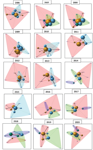
Analyzing the networks dynamically, in 2006 two groups were formed, the first encompasses France as the country with the greatest weight of links (understood as outgoing and incoming links), and which includes the Netherlands, Italy, Greece and Belgium, and the second group with the country with greater weight of links with Germany and that includes Portugal, Spain, Luxembourg, Spain, Ireland, Finland and Austria. In 2007 Belgium and Holland left the French group forming their own group, having three groups and maintaining this structure in 2008, until 2009, the year of the international financial crisis. In 2009 the groups formed are: a group formed by Austria, Italy, France and Greece and a second group by the rest of the countries with Germany as the country with the greatest weight. These two groups will remain in 2010, 2011, 2012 and 2013. With some variations such as the node/Greece, in 2011, 2012 and 2013 it leaves the French group and becomes part of the German group. Likewise, Belgium in 2010 and 2011, 2012 and 2013, moved from the Germany group to that of France. In 2014 a third group emerged, formed by Portugal and Spain, which remained in 2016, 2017, 2018 (this year Ireland joined) and 2020.

From 2014 to 2020, the two large groups formed with the two most important nodes within each of them, on the one hand, France, and on the other, Germany, continue to be maintained. In the French group, Italy, Belgium and Austria are present every year. In the group of Germany, Holland and Luxembourg are present in all years. As of 2015, it is observed that Germany ceases to be the largest node within the total network, equaling France and seeing itself surpassed, in the rest of the years until 2020. From the dynamic structure of the subnetworks, it can be seen it can be inferred that the links have been reduced from 2010 to 2017, recovering timidly from 2018 (see Figure 1).

The degree of modularity increases throughout the study period depending on the three periods (see Figure 2), which indicates greater fragmentation.

Figure 2. Modularity.

Figure 2 shows how modularity goes through three stages. The first from 2006 to 2009 is that it is low, so there are fewer subnets within the main network. In this first section, the modularity values are low, indicating that the network resembles a random network, in which the communities or subnetworks have a lower relationship with each other and a greater relationship with neighboring subnetworks. The second stage from 2010 to 2014, in which the value of modularity increases and therefore the intensity of the subnetworks, increases modularity meaning greater network fragmentation, reducing the relationship between networks and increasing intraconnectivity. Finally, the stage from 2015 to 2020 in which the intensity is accentuated to a greater degree. From these results it can be inferred how international banking integration in the eurozone has increased its fragmentation in the study period. It should be noted that the highest value occurred in 2015, which can be attributed to the great economic and political instability in Greece. This instability would be transmitted through the links, affecting the network, increasing its fragmentation.

Figure 3 represents the DT, which is defined as the sum of outgoing and incoming links at the nodes. Figure 3 shows that the countries with the highest value are Germany and France, approaching two billion. Being the two most important nodes of the network. The DI, which is defined as the input links of the nodes, Germany remains the most important country. But the countries of southern Europe, specifically Italy and Spain, occupy a central place, with Italy ahead of France (see Figure 4). As for the node that has the most outputs measured by the DO (see Figure 5), France is ahead of Germany, being the great promoter of output links. By years in Figures 4, 5 and 6, it is observed how the highest average value was produced in the years prior to the financial crisis of 2008, which was reduced from then until 2015 to begin a small rebound as of 2016. It is also observed as the data before the 2008 crisis, the distribution is symmetric to gradually become a positive symmetric distribution per year, that is, there are more and more values separated from the mean to the right or higher values in our Figure 5 Regarding the variability of the three Figures 4, 5 and 6 by years, the values show greater variability before the 2008 crisis, reducing in 2009. For DI, a cycle is observed in terms of its mean values with the peak in the years before the crisis. Crisis and its minimum values in 2015, to experience a small recovery from 2016. Regarding the distribution of the data by years in the DI figure, the distribution is presented as negative symmetric in the years of euro crisis from 2011 to 2015, for the last years from 2016 to 2020, a symmetry is observed in the data. For the DO distribution, except in the years before the 2008 financial crisis, in later years the distributions are positively symmetric.

Figure 3. Degree total.

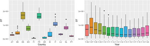
Figure 4. Degree in.

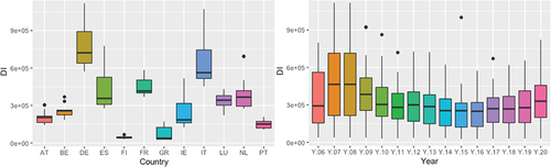
Figure 5. Degree out.

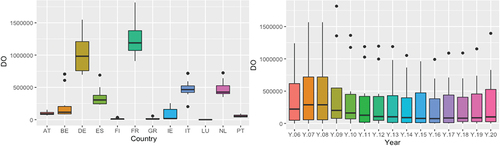
Figure 6. Betweenness.

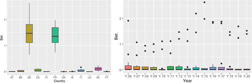
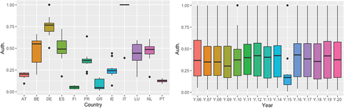
For the Betweenness measure, the two nodes that contain the greatest amount of information are France and Germany, followed by the Netherlands (See Figure 6). It is observed how in times of crisis such as 2014 or 2015, Germany and France are the nodes that act with greater intensity in a geodesic route, while the rest of the countries take lower values, presenting less deviation, as can be seen in Figure 6. Regarding the authority (see Figure 7), it is observed that Italy is a great source of information, therefore, this country is revealed as an important graph for the network, not identified with the previous measures. In 2015, in the figure by years (Figure 7), there was a sharp drop in the average, possibly caused by the Greek crisis.

Figure 7. Authority.

Next, it will be studied to what extent the increase in modularity is related to the financial characteristics of the banking systems that represent each of the nodes/countries of the network, as well as to the economic variables of each node/country. Also, in the analysis, the measurements of the network obtained previously will be introduced to observe how it is related to the modularity of the network.

Table 1 represents the variables to be studied, specifically the analysis will be carried out from the year 2008, due to the availability of the data. These variables are obtained from the European Central Bank.

Table 1. Bank variables

Bank variables	Codes
Return on assets	ROA
Return on equity	ROE
Cash and cash balances with central banks [% of total assets]	Cash.TA
Cost-to-income ratio [%]	Cost_Income_Ratio
Net interest income [% of total assets]	Net_interest_Income
Interest expenses [% of total assets]	Interest _expenses
Net fee and commission income [% of total assets]	NFC.A
Net interest income [% of total income]	NII.TI
Net fee and commission income [% of total income]	NFC.IT
Total loans and advances [% of total assets]	Total_loans_advances
Total debt securities [% of total assets]	Total_debt_securities
Total equity [% of total assets]	Total_equity
Solvency ratio [%]	Solvency_ratio
Tier 1 ratio [%]	Tier1_ratio
Tier 1 buffer [%]	Tier1_buffer
Risk-weighted assets [% of total assets]	Risk_weighted_assets
Tier 1 capital [% of own funds]	Tier1_capital. OF
Tier 1 capital [% of own funds]	Tier2_capital. OF
Total operating expenses [% of total assets]	Operating_profits

Each of the variables is averaged per year and the correlations are made (see Figure 8) in which the significant values at 95% are collected, the non-significant ones appear with a cross. Also, for those more important banking relations, an analysis will be carried out that represents other statistical measures.

Figure 8. Correlations.

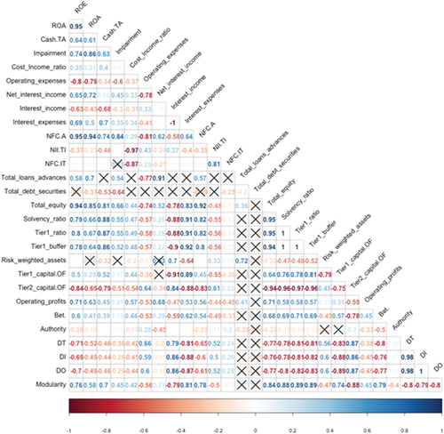
The last row of Figure 8 shows the correlations between modularity and network variables. It can be seen how there is a very strong correlation between the solvency variables (total own funds, solvency ratio, tier 1 ratio, tier 1 buffer) and the modularity and negative values with the Tier 2_capital. OF solvency ratio. The DT, DO, DI link measurements also have a very high negative correlation with network modularity. Therefore, the decline in network links coincides with increased solvency of network banking systems and correlates with increased fragmentation into subnetworks. This may confirm the theory that a network with higher intraconnectivity and lower interconnectivity may be less risky, as it can benefit from diversification within the subnetwork and reduce exposures to other subnetworks in case of systemic risk episodes.

Regarding the average measure of betweenness of the network, it is observed that it correlates positively with modularity. This is because as the modularity increases and the intra-connectivity of the subnets is greater, the betweenness measurement increases (see Figure 6), this indicates that the central value of each subnet becomes more important as the interconnectivity is reduced, that is, the relationships between networks.

Regarding interest income and expenses, it can be seen how they are negatively correlated (the interest expense ratio is represented in negative values, therefore the correlation is positive, although it expresses a negative relationship). This would indicate a reduction in the financing and investment rates on average in the network, in turn there is an increase in the NFC.A ratio (non-financial commission on assets) on average in the network throughout the period positively related to the modularity. This last positive correlation, in addition to the increase in bank commissions due to the reduction in interest income, may be due to the reduction in competition, due to less interconnectivity and the reduction in incoming links.

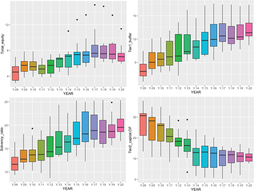
Figure 9 shows how the total equity ratio increases throughout the study period, with relevance to the higher quality Tier 1 reserve capital, as well as the solvency ratio, and the lower quality Tier 2 on equity, decreases throughout the period.

Figure 9. Regulatory ratios.

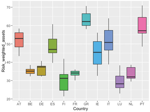
Regarding liquidity over total assets, it is observed that in the study period it has a positive trajectory, therefore, the banking nodes/systems of the countries, in the communities increase their liquidity positions, fewer investments are made (see Figure 10). Risk-weighted assets, although they show a negative correlation in Figure 8, where their change is most appreciated together with the increase in modularity is the narrowing of their interquartile range. Also, in the decrease of the dispersion of the values above the median. In fact, in recent years the dispersion between the first quartile and the median, and between the median and the third quartile, has become equal. Therefore, there is a reduction in risk in the network, since the third quartile greatly reduces its variability, especially as of 2014, as can be seen in Figure 11. Correlation Figure 8 shows how risk-weighted assets are positively correlated with DI and DO, that is, outgoing and incoming links.

Figure 10. Cash over total assets.

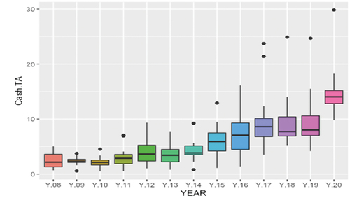
Figure 11. Risk weighted assets per year.

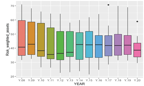
By country, it should be noted that the two nodes with the highest Betweenness, Germany and France, are among the nodes with the lowest risk-weighted asset values (see Chart 12). As for the risk in its risk-weighted assets by country (see Chart 12), it stands out that Austria, Spain, Greece, Ireland and Portugal are all above 40% practically during the entire study period. While the countries with the lowest risk, Belgium, Germany, Finland, France, Luxembourg and the Netherlands, are below 40% during the entire study period. Therefore, it can be said that together with the lower modularity, the opportunities for investment diversification were reduced by concentrating more on the communities themselves. Overall, risk taking, as measured by risk-weighted assets in the network during the study period, has decreased.

2.3. Data and machine learning methodology

In this section, an analysis of the determinant variables of the outgoing and incoming links in the nodes is carried out. This analysis seeks to identify the push and pull variables of international banking flows in the euro zone. For this, the output and input links of the analyzed networks are used. Due to the disposition of the data, the analysis is carried out from 2008 to 2020, with the same countries as in the previous analysis. The push and pull variables will be determined by machine learning algorithms, specifically regression trees and random forest. Due to the complexity of this last algorithm, mathematical statistical techniques are used that will allow us to interpret its results.

The push and pull variables will be studied from two categories, a first category that encompasses the analysis of the variables that catalog the banking systems of each of the countries, that is, the flow conduits, and a second category that encompasses the economic variables of the countries.

This will produce four sets of variables: i) push bank variables, ii) push economic variables, iii) pull bank variables and pull economic variables.

To do this, the same banking variables (Table 1) from the previous section and economic variables (Table 2) presented below are taken as dependent variables. As independent variables, the outgoing and incoming links of each country/node of the network from the previous section are taken, weighted by the total banking assets of each node. Due to the availability of data on the banking and economic variables of each node/country, the study is carried out from 2008 to 2020.

Table 2. Economic variables

Economic variables	Codes
Productivity per hours worked	Productivity
Population change - crude rates of total change, natural change and net migration plus adjustment	Grow_pop.
Gross domestic product at market prices converted using purchasing power parities; ratio to total population.	GDP
Balance (Credits minus Debits)- Current account- Euro; ratio to gross domestic product.	Balance_payments
Government debt (consolidated) (as % of GDP)	Debt
Unemployment	Umployment
Inflation	Inflation
Residential property, All dwelling types, new and existing. Transaction value - actual or estimated based on other types of values, e.g., appraisals, Deflated by the private consumption deflator. Unit, 2015=100.	Property prices

To carry out the analysis, regression trees and random forest are used. A regression tree is used ,⁵ which is a machine learning method to build prediction models from data. As advantages, they present an easy interpretation and their robustness to extreme values. It also enables capturing linear and non-linear relationships and there may be a link between variables. As problems, this methodology presents a remarkably high variance, that is, a small change in the data can cause different partitions of the data. This will be corrected using different Machine Learning ensemble methods such as the random forest model (the advantages of random forest in addressing the variance issue are presented in Annex 1). The regression tree follows the following model:

Let Y be a response variable and let p be predictor variables x1, x2, …, xp, where the xs are taken fixed and Y is a random variable. The statistical problem is to establish a relationship between Y and the X’s in such a way that it is possible to predict Y based on the values of the X’s. To do this, we want to estimate the function of its probability such as:

$\mathrm{E}\left[\mathrm{Y}|{\mathrm{x}}_1,{\mathrm{x}}_2,..,{\mathrm{x}}_{\mathrm{p}}\right]$

It seeks to obtain a minimum variance within each node τ of the tree,

$\mathrm{i}\left(\tau \right)={\sum }_{i\in \tau }{\left({\mathrm{Y}}_{\mathrm{i}}-{\mathrm{Y}}_{(\tau )}\right)}^2$

Where Y (τ) is the average of Y ́s within the node τ.

To divide a node τ into two child nodes, τ_L (left node) and τ_R (right node), the goodness of a division s is defined as:

$\mathrm{\Delta }\mathrm{I}\left(\tau \right)=\mathrm{i}\left(\tau \right)-\mathrm{i}\left({\tau }_{\mathrm{L}}\right)-\mathrm{i}\left({\tau }_{\mathrm{R}}\right)$

With this last equation, the impurity reduction is obtained when the parent node is passed to the child node, the impurity reduction is sought to be maximum.

The objective is to obtain the maximum homogeneity of those of the terminal nodes.

It is sought that R (τ) be minimized as:

$\mathrm{R}\left(\tau \right)={\sum }_{\tau \in \zeta }\mathrm{i}\left(\tau \right)$

Where ζ represents the set of terminal nodes.

A random forest is an algorithm that has the following advantages: in prediction trees like all statistical models, the balance between bias and variance must be taken into account. By the concept of bias, it is understood how far the predictions from the real values are on average. Variance is understood as the variation of the model, depending on the sample used in the training phase. More complex models tend to reduce bias, increasing the predictability of the model. On the other hand, an overfit can occur, that is, the model adjusts so much to the training data that it does not correctly predict new data. Therefore, a model with a balance between bias and overfit is pursued.

In predictive tree models with many nodes, they tend to fit the training sample very well, but at the cost of greater variance. With the assembly method used in this work, a balance between bias and variance is pursued. In the method of Random Forest,⁶ repeated sampling is carried out. A model is fitted with the different samples of the population, and the result is averaged, reducing the variance. For this, bootstrapping is used, generating different samples through resampling). With each of these samples a tree is made, which is not pruned, having a reduced bias but a greater variance. The algorithm’s stop system is the minimum number of observations that the final nodes must have. It is a modification of the bagging model by mitigating the correlation between the trees; this is achieved by selecting the predictors at random. It prevents a very influential predictor from dominating the construction of the trees and allows other predictors to be evaluated in the construction of the trees.

The MSE estimates the prediction error of the model considering these observations that have been “left out of the training sample”. This error is calculated as follows: $\frac{1}{n}{\mathrm{\Sigma }}_{i=1}^n{\left(\mathrm{y}\mathrm{i}-\mathrm{y}\mathrm{i}\mathrm{O}\mathrm{O}\mathrm{B}\right)}^2$

Being $y{i}_{OOB}$ the prediction for observation is obtained by averaging the individual predictions of the trees for which that observation has been left out of the training sample and real the actual value of the response variable.

To calculate the importance of the predictors, the increase in the MSE and the increase in the purity of the nodes are used. The increase in the MSE identifies the influence of each predictor on the MSE of the model estimated by the out of bag error.

$\mathrm{M}\mathrm{S}\mathrm{E}\mathrm{O}\mathrm{O}\mathrm{B}(\mathrm{X}\mathrm{j}\mathrm{p}\mathrm{e}\mathrm{r}\mathrm{m}\mathrm{u}\mathrm{t}\mathrm{e}\mathrm{d})=\frac{1}{n}{\mathrm{\Sigma }}_{i=1}^n\left(\mathrm{y}\mathrm{i}-\mathrm{y}\mathrm{i}\mathrm{O}\mathrm{O}\mathrm{B}\right){(\mathrm{X}\mathrm{j}\mathrm{p}\mathrm{e}\mathrm{r}\mathrm{m}\mathrm{u}\mathrm{t}\mathrm{e}\mathrm{d})}^2$

After this, for each variable $X$ in each tree t, the difference between the two measures MSE OOB ($\mathrm{X}\mathrm{p}\mathrm{e}\mathrm{r}\mathrm{m}\mathrm{u}\mathrm{t}\mathrm{e}\mathrm{d}$) and MSE OOB is calculated. This difference, for each variable, is summed in all the trees, averaged and normalized between the standard deviation of the differences. The result of this process is a measure of the importance of each variable. If the predictor that is not included provides information about the model, the MSE will increase.

The increase in the purity of the nodes is calculated by the decrease in the MSE, which is calculated as the average decreases. Therefore, the higher the value, the greater the contribution of the predictor to the model.

Next, the regression trees are developed and subsequently the random forest to determine the banking and economic variables in the outflows of funds (granting credits abroad) and the inflows of funds (granting credits to the interior). Also, in the random forest, different methods are used in the interpretation of the results of the variables. Also, in the random forest, different methods are used in the interpretation of the results of the variables. Specifically, the functions of partial derivatives and alluvial graphs.

2.4. Analysis of bank push variables

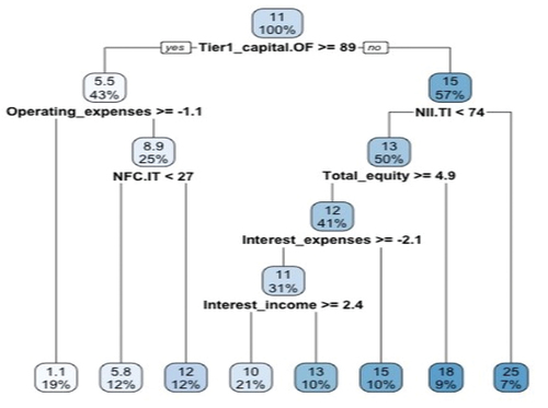
Figure 12 shows the regression tree on the dependent variable outputs, that is, the loans granted from each node/country to the rest of the nodes/countries.

Figure 12. Risk weighted assets per country.

The regression tree shows that the most important variable is TIER1 capital over equity, which is the most determining variable. When this ratio is not greater than or equal to 89%, the outputs represent an average of 15%. While when it is greater than 89%, the outputs represent an average of 5.5%. It can be inferred that for very high values of this ratio, banking systems make fewer loans to other countries. Therefore, when own funds approach higher quality capital, the activity of granting loans to other entities, in other European jurisdictions, is less. This may be due to stricter regulatory criteria regarding the quality of capital. In the second division of the tree, when the interest margin on total income is greater than 74%, the largest outflows occur, with a value of 25%.

On the other hand, for smaller amounts of expenses, we have operating expenses over total assets. In the first level branch, own funds greater than 89% and operating expenses greater than −1.1, that is, with lower operating expenses over total assets, there are fewer outflows of funds, this fact may be due to less activity.

In the final sections, when the equity coefficient is greater than or equal to 4.9 (see Figure 13), the outputs are lower (values 13) than when they are less than 4.9 (values 19). Indicating that leverage plays in favor of exits.

Figure 13. Regression tree (bank push variables).

The RMSE or root mean square error, as it is not linear, gives greater weight to larger errors and is interpreted as:

$\sqrt[2]{\frac{1}{n}}{\sum }_{j=1}^n{\left(y_j-\widehat{y_j}\right)}^2$

The MAE or mean absolute error is linear and all errors are weighted equally and interpreted as:

$\frac{1}{n}{\sum }_{j=1}^n\left|\left(y_j-\widehat{y_j}\right)\right|$

The RMSE when making the squares of the errors is penalizing the outliers more. Therefore, the MSE from this last point of view would be more robust. The table shows how the random forest improves the predictions in the regression tree. For this, the models have been trained on 80% of the sample and the remaining 20% have been evaluated, obtaining improvements in the prediction with the random forest as observed for all the models (see Annex 2)

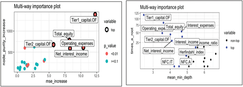
For the random forest, the most important variable in determining outflows is Tier 1 over equity (see Annex 3).

In the alluvial flow diagram, it is a method based on Sankey diagrams⁷ with which we interpret random forest models. First, the dependent numeric variable, are transformed into 5 bins of equal rank, which are filled with “LL” (low-low), “ML” (medium-low), “M” (medium), “MH” (medium high), HH (high-high) by default. On the x-axis the variable pred. represents the dependent variable. The dependent variables are represented in the following columns. In each rectangle of the independent variables, the five codes established in the independent variable and the percentage of each of the five scales of the dependent variable that passes through each dependent variable are presented. Each dependent variable in turn in the graph is divided into 4 boxes that categorize the data, showing in each of them the average that it reaches with the values in ascending order. For example, in the first dependent variable (Tier 1 on own funds) the values of LL (dependent variable) are distributed by 0.53 in the highest values of Tier 1 on own funds with a mean of 105.7, and the 0.43 remaining in the second highest values of the same dependent variable with a mean value of 99.7. The graph of alluvial colors shows the relationship between the variables (see Figure 14), specifically it is observed that the pink color that starts from the low values of the output variable (interval of 3.41 and 6.67), is related to high values of TIER1 on own funds, as well as with high and intermediate values of the ratio of total own funds. As well as with high values of operating expenses, following the pink lines. The pink graph indicates that high values of tier 1 capital to capital and of the capital ratio, as well as operating expenses are related to each other, as well as low values of expenses. On the other hand, the dark brown and blue plot indicates the opposite, that is, high values of the outputs are related to low values of the three dependent variables, which first appear indicating an inverse relationship in the random forest model. Therefore, in the banking systems analyzed, when the capital and highest-quality capital ratios are high, the banking systems grant fewer loans abroad, there are fewer outflows, operating expenses in these circumstances are lower, and vice versa. These relationships are shown as shown in Figure 15 with the partial derivative functions.

Figure 14. Alluvial (bank push variables).

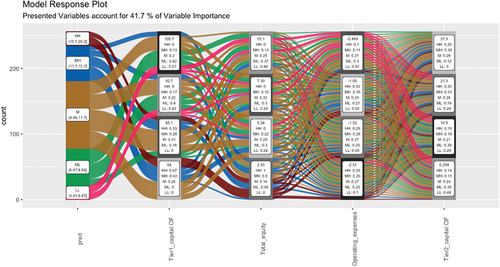
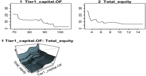
Figure 15. Partial derivatives (bank push variables).

2.5. Analysis of bank pull variables

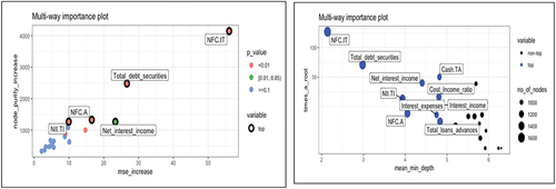
Figure 16 shows the regression tree on the dependent variable inputs, that is, the loans granted to each node from the rest of the nodes. It is observed how the variable NFC.IT represents the most important variable, specifically when commission income exceeds 41% of total income, the largest inflow of funds via loans is presented. Between 30 and 40%, the lowest inflows of funds occur. For values less than 30%, there is an intermediate inflow of loans (an average of 19%). These results can be explained by the fact that when commissions occupy a very high percentage of revenue, then the interest margin has less weight on total revenue. This may be an indication of low competition; it may also be an indication of great dynamism in the national market. Therefore, investment opportunities are sought in these markets. On the other hand, when the structure of total income, on commissions, represents between 30% and 40%, the inflows are lower because they correspond to banking systems with greater competition. For low values of commissions over total income, the banking markets would appear in a low phase of the cycle or with high competition, which would mean investment searches in other markets. The second important variable in the regression tree that appears is the debt assets over total assets, when it takes values less than 21, fewer bank loans are generated with an average of 16%, for values greater than 21 the inputs represent 33%. Therefore, when banking markets increase their investments in debt assets, they occur in growth environments, in which companies borrow with the intention of undertaking new investment projects, and in turn, international loans reach these economies.

Figure 16. Regression tree (bank pull variables).

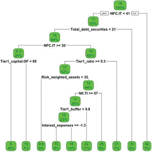
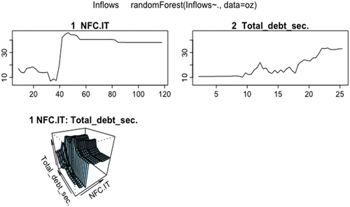
Annex 4 shows how the most important variables are NFC. TI and total debt titles. The Alluvial graph (see Figure 17) shows how there is a direct relationship between the inflows and the NFC.IT variable and the Total Debt Securities variable. When commissions are high over total income, either due to less competition or a greater number of operations due to a more favorable phase of the cycle, the inflows are higher. As for the total debt securities variable, the direct relationship is explained by a better phase of the cycle with higher debt issues and higher inflows for its financing. Figure 18 shows the graphs of partial derivatives of both variables with respect to the inputs.

Figure 17. Alluvial (bank pull variables).

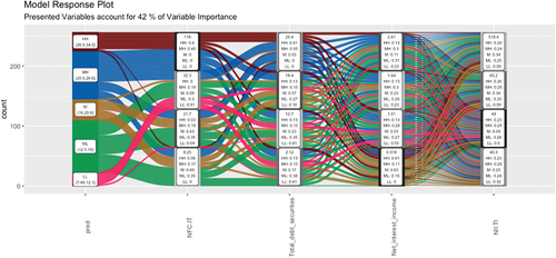
Figure 18. Partial derivatives (bank pull variables).

2.6. Analysis of economic push variables

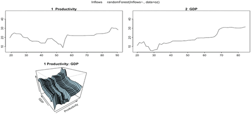
Figure 19 shows how the greater the productivity, the granting of credits abroad is very low, specifically at 0.81. For lower values of productivity 60, the granting of credits abroad, are higher, taking values of 13. In the next branch, the population growth is found, when it is less than 0.48%, the granting of credits is lower, with values of 11, for values higher than 0.48%, on average, the granting of loans is situated in average values of 16. In the next branch that comes from the latter, there is a greater granting of loans, when the GDP is lower than 36.

Figure 19. Regression tree (economic push variables).

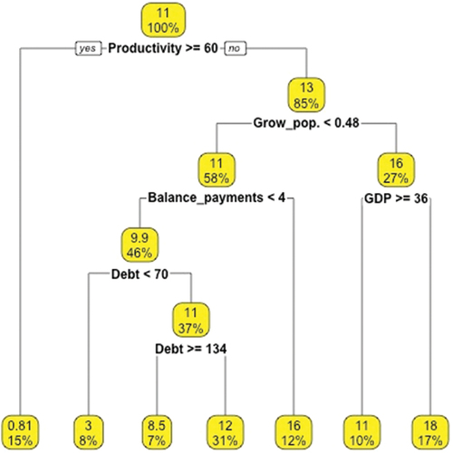
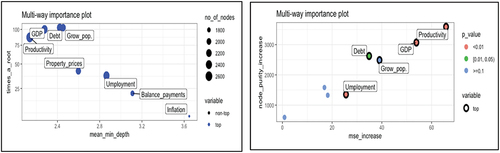
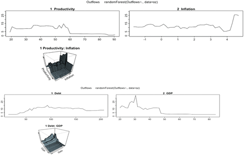
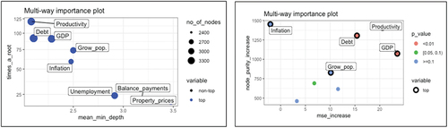
Productivity, debt and GDP appear (see Annex 5) as the most important variables. Specifically, with the Alluvial graph (see Figure 20) a negative relationship between outflows and productivity is observed. While the relationship is direct with inflation for high values of it. Therefore, in an economy with high productivity, outputs are lower, as well as when inflation is high. It is assumed that when productivity is low, more investment opportunities are sought in other countries. Figure 21 shows that for GDP values greater than 47, the outflows are greatly reduced, which indicates that for high-growth economies they require more financing and their outflows are smaller.

Figure 20. Alluvial (economic push variables).

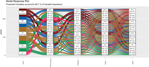
Figure 21. Partial derivatives (economic push variables).

2.7. Analysis of economic pull variables

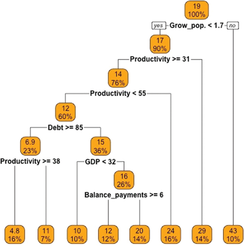
In the regression tree (Figure 22) the first variable that appears is population growth, for values of this variable greater than 1.7, the largest international loan concessions are produced with values of 43. This would occur because we would be in economies that produce wealth, increasing their workforce and creating families or receiving immigration. The second variable in the division in the tree is productivity, for values greater than or equal to 31 there is a lower credit output, specifically the average is 14 and for productivity values less than 31 the credit output takes a value of 29. Between 50 and 31 productivity, the average loan takes values of 12. For productivity values greater than 55, the average granting of loans abroad is 24. This fact indicates that when productivity is low, the greater granting of loans. This may occur due to fewer investment opportunities due to lower productivity values. But for high productivities there is also a large granting of loans, this may be due to greater competition in the markets than for intermediate productivities, in which there are fewer outflows of funds via loans.

Figure 22. Regression tree (economic push variables).

Productivity is once again the most important variable in entries, followed by the GDP variable (see Annex 6). According to the Alluvial chart (see Figure 23), the relationship between productivity and loan inflows is direct, as well as for higher GDP growth rates. As the graph of the functions of partial derivatives Figure 24 is observed.

Figure 23. Alluvial (economic pull variables).

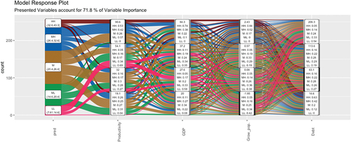
Figure 24. Partial derivatives (economic pull variables).

3. Conclusions

In the work complex networks are used to analyze interbank loans in the euro zone. It is concluded that fragmentation in the euro area has been increasing in the euro area between 2006 and 2020, identifying three phases in which fragmentation gradually increases. The turning points in the increase in fragmentation coincide with crisis events.

The topology of the networks, weighted by the outgoing and incoming links, shows a clear center formed by Germany and France, with the former losing prominence in favor of the latter throughout the study period. According to network measurements, Germany and France are the largest information managers in the network, although as the largest source of information the most important node/country is Italy.

The measure of fragmentation in the modularity network shows a positive correlation with the solvency measures. The subnets that are formed have a lower risk measured by the solvency of the nodes and by the assumption of risks. Higher fragmentation is also associated with higher liquidity at the nodes.

As policy implications, there is greater security in the network due to its greater solvency and lower assumption of risk together with greater fragmentation. The analysis could be useful for combining euro zone banking regulation, supervision and integration with network and sub-network risk.

It is concluded that solvency is the most determining variable for the outflow of bank flows with an indirect relationship and the income structure measured by the ratio of commissions to total income is the most determining variable for the inflow of funds. The most solvent banking systems would be less willing to take risks in other jurisdictions and, if this is the case, it would be in banking systems with less competition and/or an expanding banking market.

It is concluded that from an economic perspective, productivity differentials are the main determinants of bank flows in the euro zone, increasing the receipt of funds and decreasing outflows in a country with high productivity.

Disclosure statement

No potential conflict of interest was reported by the author(s).

Notes

1. REGULATION (EU) No 575/2013 OF THE EUROPEAN PARLIAMENT AND OF THE COUNCIL of 26 June 2013 on prudential requirements for credit institutions and investment firms and amending Regulation (EU) No 648/2012.

2. Examples of some of these works can be found in Amini et al. (2012), Acemoglu et al. (2015), Battiston et al. (2012), and Caccioli et al. (2012).

3. McGuire and Wooldridge (2005), Muñoz de la Peña and Rixtel (2015) and the Basel Committee (2019) develop different advantages and disadvantages of collecting bank data from different perspectives of the BIS databases.

4. In Figure 1, the topological structures of the European Union’s banking systems are presented, grouped by clusters and according to the years of study.

5. The strengths and weaknesses of the regression trees is developed by Loh (2011) and the development of the algorithm by Breiman et al. (1984).

6. Breiman (2001) develops the advantages of random forest.

7. Sankey diagrams are developed and explained by Riehmann et al. (2005) and Lupton and Allwood (2017)

Annex 1.

Appendices

Random Forest

The Random Forest algorithm offers several benefits for reducing variance. Among the key advantages of Random Forest in addressing variance are the aggregation of multiple decision trees. By combining the predictions of multiple decision trees, Random Forest reduces the impact of individual trees that may overfit or have high variance. Therefore, the ensemble model tends to provide more stable and reliable predictions.

Additionally, the algorithm introduces random feature subsampling. In other words, Random Forest introduces randomness by considering only a random subset of features at each split when constructing individual decision trees. This randomness feature reduces the risk of overfitting and helps the model generalize better. By considering different subsets of features, Random Forest captures a more diverse range of information from the data, leading to reduced variance.

Random Forest utilizes the sampling technique called bootstrapping, which involves randomly extracting subsets of the training data with replacement to train each decision tree. This sampling strategy introduces diversity in the training data for each tree, contributing to variance reduction. By constructing different data subsets for each tree, it allows the ensemble to capture a wider range of patterns and reduces the likelihood of overfitting.

Therefore, Random Forest aggregates the predictions of all decision trees in the ensemble by taking the average. This averaging process helps smooth out individual errors and reduces the impact of outliers or noise in the predictions. By combining multiple predictions, the ensemble model becomes more robust and less prone to high variance.

Annex 2.

Models

Table

MODELS	RMSE	MAE
PUSH BANK REGRESSION TREE	7,158	4,607
PUSH BANK RAMDON FOREST	2,146	1,198
PULL BANK REGRESSION TREE	8,717	6,639
PULL BANK RAMDON FOREST	7,764	6,143
PUSH ECONOMIC REGRESSION TREE	5,234	4,086
PUSH ECONOMIC RAMDON FOREST	1,751	1,226
PULL ECONOMIC REGRESSION TREE	7,551	4,721
PULL ECONOMIC RAMDON FOREST	5,243	4,236

Annex 3.

Graphs of variables of importance (bank push variables)

Annex 4.

Graphs of variables of importance (bank pull variables)

Annex 5.

Graphs of variables of importance (Economic push variables)

Annex 6.

Graphs of variables of importance (Economic push variables)

References

- Abduraimova, K., & Nahai-Williamson, P. (2021). Solvency distress contagion risk: Network structure, bank heterogeneity and systemic resilience. Staff Working Paper No. 909, Bank of England.
- Acemoglu, D., Ozdaglar, A., & Tahbaz-Salehi, A. (2015). Systemic risk and stability in financial networks. American Economic Review, 105(2), 564–30. https://doi.org/10.1257/aer.20130456
- Allen, F., & Gale, D. (2000). Financial contagion. Journal of Political Economy, 108(1), 1–33. https://doi.org/10.1086/262109
- Amini, H., Cont, R., & Minca, A. (2012). Stress testing the resilience of financial networks. International Journal of Theoretical and Applied Finance, 15(1), 1250006. https://doi.org/10.1142/S0219024911006504
- Basel Committee. (July 2019). Reporting guidelines for the BIS international banking statistics. Monetary and Economic Department
- Battiston, S., Gatti, D., Gallegati, M., Greenwald, B., & Stiglitz, J. E. (2012). Liaisons dangereuses: Increasing connectivity, risk sharing, and systemic risk. Journal of Economic Dynamics and Control, 36(8), 1121–1141. https://doi.org/10.1016/j.jedc.2012.04.001
- Benigno, G., Converse, N., & Fornaro, L. (2015). Large capital inflows, sectoral allocation, and economic performance. Journal of International Money and Finance, 55, 60–87. https://doi.org/10.1016/j.jimonfin.2015.02.015
- Bhattacharya, M., Inekwe, J. N., & Valenzuela, M. R. (2020). Credit risk and financial integration: An application of network analysis. International Review of Financial Analysis, 72, 101588. https://doi.org/10.1016/j.irfa.2020.101588
- Breiman, L. (2001). Random forests. Machine Learning, 45(1), 5–32. https://doi.org/10.1023/A:1010933404324
- Breiman, L., Friedman, J., Olshen, R., & Stone, C. (1984). Cart. Classification and regression trees (1st ed.). Routledge. https://doi.org/10.1201/9781315139470
- Brunetti, C., Harris, J. H., Mankad, S., & Michailidis, G. (2019). Interconnectedness in the interbank market. Journal of Financial Economics, 133(2), 520–538. https://doi.org/10.1016/j.jfineco.2019.02.006
- Caballero, J. (2015). Banking crises and financial integration: Insights from networks science. Journal of International Financial Markets, Institutions and Money, 34, 127–146. https://doi.org/10.1016/j.intfin.2014.11.005
- Caballero, J. (2016). Do surges in international capital inflows influence the likelihood of banking crises? The Economic Journal, 126(591), 281–316. https://doi.org/10.1111/ecoj.12172
- Caccioli, F., Catanach, T. A., & Farmer, J. D. (2012). Heterogeneity, correlations and financial contagion. Advances in Complex Systems, 15(supp02), 1250058. https://doi.org/10.1142/S0219525912500580
- Cingano, F., & Hassan, F. (2020). International financial flows and misallocation. CEP Discussion Paper, no 1697, Centre for Economic Performance.
- Committee on the Global Financial System. (2021) Changing patterns of capital flows. CGFS Papers No 66.
- Cont, R., & Moussa, A. (2010). Network structure and systemic risk in banking systems. Edson Bastos E, Network Structure and Systemic Risk in Banking Systems (December 1, 2010).
- Dasgupta, A. (2004). Financial contagion through capital connections: A model of the origin and spread of bank panics. Journal of the European Economic Association, 2(6), 1049–1084. https://doi.org/10.1162/1542476042813896
- Detering, N., Meyer-Brandis, T., Panagiotou, K., & Ritter, D. (2019). Managing default contagion in inhomogeneous financial networks. SIAM Journal on Financial Mathematics, 10(2), 578–614. https://doi.org/10.1137/17M1156046
- Devereux, M. B., & Yu, C. (2020). International financial integration and crisis contagion. The Review of Economic Studies, 87(3), 1174–1212. https://doi.org/10.1093/restud/rdz054
- Emter, L., Schmitz, M., & Tirpák, M. (2019). Cross-border banking in the EU since the crisis: What is driving the great retrenchment? Review of World Economics, 155(2), 287–326. https://doi.org/10.1007/s10290-019-00342-5
- European Central Bank, Committee on Financial Integration. (2022). Financial integration and structure in the euro area.
- Fabiani, J., Fidora, M., Setzer, R., Westphal, A., & Zorell, N. (2021). Sudden stops and asset purchase programmes in the euro area. European Central Bank.
- Forbes, K., Fratzscher, M., Kostka, T., & Straub, R. (2016). Bubble thy neighbour: Portfolio effects and externalities from capital controls. Journal of International Economics, 99, 85–104. https://doi.org/10.1016/j.jinteco.2015.12.010
- Forster, K., Vasardani, M. A., & Ca’zorzi, M. (2011). Euro area cross-border financial flows and the global financial crisis. ECB occasional paper, (126).
- Freixas, X., Parigi, B. M., & Rochet, J. C. (2000). Systemic risk, interbank relations, and liquidity provision by the central bank. Journal of Money, Credit and Banking, 32(3, Part 2), 611–638. https://doi.org/10.2307/2601198
- Gai, P., & Kapadia, S. (2010). Contagion in financial networks. Proceedings of the Royal Society A: Mathematical, Physical and Engineering Sciences, 466(2120), 2401–2423. https://doi.org/10.1098/rspa.2009.0410
- Georg, C. P. (2013). The effect of the interbank network structure on contagion and common shocks. Journal of Banking & Finance, 37(7), 2216–2228. https://doi.org/10.1016/j.jbankfin.2013.02.032
- Gopinath, G., Kalemli-Özcan, S., Karabarbounis, L., & Villegas-Sanchez, C. (2017). Capital allocation and productivity in South Europe. The Quarterly Journal of Economics, 132(4), 1915–1967. https://doi.org/10.1093/qje/qjx024
- Hazell, J., & Elliott, M. (2016). Endogenous financial networks: Efficient modularity and why shareholders prevent it. In 2016 Meeting Papers (No. 235). Society for Economic Dynamics.
- Huang, Y., & Chen, F. (2021). Community structure and systemic risk of bank correlation networks based on the US financial crisis in 2008. Algorithms, 14(6), 162. https://doi.org/10.3390/a14060162
- Inekwe, J. N., & Valenzuela, M. R. (2020). Financial integration and banking crisis. A critical analysis of restrictions on capital flows. The World Economy, 43(2), 506–527. https://doi.org/10.1111/twec.12855
- Jappelli, T., & Pistaferri, L. (2011). Financial integration and consumption smoothing. The Economic Journal, 121(553), 678–706. https://doi.org/10.1111/j.1468-0297.2010.02410.x
- Kose, M. A., Prasad, E., Rogoff, K., & Wei, S. J. (2009). Financial globalization: A reappraisal. IMF Staff Papers, 56(1), 8–62. https://doi.org/10.1057/imfsp.2008.36
- Ladley, D. (2013). Contagion and risk-sharing on the inter-bank market. Journal of Economic Dynamics and Control, 37(7), 1384–1400. https://doi.org/10.1016/j.jedc.2013.03.009
- Lambert, F., & Ichiue, H. (2016). Post-crisis international banking: An analysis with New regulatory Survey data (No. 2016/088). International Monetary Fund.
- Lane, P. R. (2013). Capital flows in the euro area. Economic Papers 497 | April 2013. European Commission.
- Lenzu, S., & Tedeschi, G. (2012). Systemic risk on different interbank network topologies. Physica A: Statistical Mechanics and Its Applications, 391(18), 4331–4341. https://doi.org/10.1016/j.physa.2012.03.035
- Loh, W. Y. (2011). Classification and regression trees. Wiley interdisciplinary reviews: Data mining and knowledge discovery. WIREs Data Mining and Knowledge Discovery, 1(1), 14–23. https://doi.org/10.1002/widm.8
- Lupton, R. C., & Allwood, J. M. (2017). Hybrid Sankey diagrams: Visual analysis of multidimensional data for understanding resource use. Resources, Conservation and Recycling, 124, 141–151. https://doi.org/10.1016/j.resconrec.2017.05.002
- Mancoridis, S., Mitchell, B. S., Rorres, C., Chen, Y., & Gansner, E. R. (1998, June). Using automatic clustering to produce high-level system organizations of source code. Proceedings of the 6th International Workshop on Program Comprehension. IWPC’98 (Cat. No. 98TB100242), Ischia, Italy (pp. 45–52). IEEE.
- McGuire, P., & von Peter, G. (2016, March). The resilience of banks’ international operations. BIS Quarterly Review, March, 65–78.
- McGuire, P., & Wooldridge, P. D. (2005, September). The BIS consolidated banking statistics: Structure, uses and recent enhancements. BIS Quarterly Review, September, 73–86.
- Muñoz de la Peña, E. A., & Rixtel, A. V. (2015). The BIS international banking statistics: Structure and analytical use. Estabilidad financiera Nº 29 (noviembre 2015), 29, 29–46.
- Reinhardt, D., & Sowerbutts, R. (2015). Regulatory arbitrage in action: Evidence from banking flows and macroprudential policy. Working Paper No. 546. Bank of England.
- Riehmann, P., Hanfler, M., & Froehlich, B. (2005, October). Interactive Sankey diagrams. In IEEE Symposium on Information Visualization, 2005. INFOVIS 2005. (pp. 233–240). IEEE. https://doi.org/10.1109/INFVIS.2005.1532152
- Stiglitz, J. E. (2010). Risk and global economic architecture: Why full financial integration may be undesirable. American Economic Review, 100(2), 388–392. https://doi.org/10.1257/aer.100.2.388
- Tarashev, N., Avdjiev, S., & Cohen, B. (2016). International capital flows and financial vulnerabilities in emerging market economies: Analysis and data gaps.