On a robust estimation of option-implied interest rates and dividend yields

Abstract

In this paper, a simple no-arbitrage methodology to estimate option-implied interest rates and dividend yields simultaneously via a regression model is employed. Since the mean-based least squares estimation places equal weights on all data points making it sensitive to outliers, a robust median-based estimation approach is proposed. The proposed methodology is only valid for European options; consequently, an empirical analysis is conducted on options on the S & P 500 Index. Robust forward-looking model-free estimates of the risk-free interest rate and dividend yield, based exclusively on market prices of options, are thus obtained.

Keywords:

• no-arbitrage
• implied interest rates
• implied dividend yield
• option-implied
• risk-free rate
• Theil–Sen
• repeated median
• box spread
• sloped asset position

1. Introduction

It is often implied that market prices of options have rich information content such as implied volatilities, risk-neutral distributions, interest rates, dividends, and dependence measures that market practitioners can extract and use in practice. Given option prices, the information is extracted either via a model-based or a model-free approach (or both).

In this paper, we employ a model-free approach constructed from simple no-arbitrage relationships and extract both option-implied interest rates and dividend yields. The no-arbitrage methodology of extracting information is not new to the literature. With regard to option-implied interest rates, Brenner and Galai (1986) extracted implied interest rates by simply rearranging the put-call parity relation. Similar approaches have also been considered by Geck and Kaserer (2021), Naranjo (2009), and Golez (2014). For a dividend paying security, however, this approach requires one to estimate, with some degree of accuracy, the dividend component contained in the put-call parity equation (2)(2) $C_{t,T}-P_{t,T}=(S_t-Q_{t,T})-K{e}^{-r_{t,T}\tau }.$(2) . To overcome this drawback, Ronn and Ronn (1989) considered the box spread, whose equation is independent of the underlying asset price, and obtained the implied risk-free interest rate by simply rearranging the box spread equation (4)(4) $C_{K_1}-C_{K_2}+P_{K_2}-P_{K_1}=(K_2-K_1)e^{-r_{t,T}\tau }\Rightarrow \frac{C_{K_1}-C_{K_2}+P_{K_2}-P_{K_1}}{(K_2-K_1)}=e^{-r_{t,T}\tau }.$(4) . This has been extended, recently, by van Binsbergen et al. (2022).

For the dividend estimation, estimates can also be obtained via a simple rearrangement of the put-call parity relation, see, for example, van Binsbergen et al. (2012) and Golez and Jackwerth (2022). However, under this approach, one has to first estimate the interest rate in the put-call parity equation. For example, van Binsbergen et al. (2012) used zero-coupon interest rates, Golez and Jackwerth (2022) used option-implied interest rates, and Golez (2014) used a combination of the cost-of-carry formula for index futures and the put-call parity for index options.

To avoid an interest rate estimation, Söderbäck et al. (2022) proposed the sloped asset position, whose resulting equation (7)(7) $\frac{K_2(C_{K_1}-P_{K_1})-K_1(C_{K_2}-P_{K_2})}{K_2-K_1}=(S_t-Q_{t,T}).$(7) does not require an interest rate specification.

In this paper, we build on the recent work by Desmettre et al. (2017), van Binsbergen et al. (2022), and Söderbäck et al. (2022) and employ a simple no-arbitrage methodology to estimate option-implied interest rates and dividend yields simultaneously via a regression model. In Desmettre et al. (2017), the ordinary least squares (OLS) estimation is undertaken to simultaneously estimate the implied discrete dividends and the implied discount factor, whereas in the study by Söderbäck et al. (2022), the dividend estimation is generalized in the form of a weighted least squares approach. On the other hand, in the estimation of the risk-free rate, van Binsbergen et al. (2022) considered the OLS and the Theil–Sen estimator. The approach proposed herein highlights, builds upon, and consolidates concepts within the studies of Desmettre et al. (2017), van Binsbergen et al. (2022), and Söderbäck et al. (2022). Consequently, the aforementioned estimators are derived in a slightly different approach.

The aim of this paper is to, one, clearly demonstrate the link between the no-arbitrage relationships between call and put prices presented in Section 2 and the estimation techniques employed in estimating both the interest rate and dividend yield, and two, to extend the estimation methodology to a more robust approach—the repeated median. Compared to the OLS estimator, the Theil–Sen and repeated median estimators are less sensitive to contamination, with the former having a breakdown point of about 29% and the latter of 50% implying higher robustness even if half the data is contaminated, Siegel (1982). The three estimators for the slope and intercept are derived from first principles via the no-arbitrage relationship, clearly demonstrating the link between the sloped asset position with the intercept and the box spread with the slope. Finally, an empirical analysis is performed on S&P 500 Index options data.

The rest of the paper is organized as follows: Section 2 provides a theoretical background of the no-arbitrage relationships to be used throughout the paper, Section 3 derives the interest rate estimators, Section 4 derives the dividend yield estimators, Section 5 provides a description of the data used, the empirical results obtained, and a discussion of the results; and, Section 6 concludes.

2. Preliminaries

2.1. Put-call parity

The put-call parity is a simple no-arbitrage relationship that exists between the prices of European call and put options on the same underlying asset with the same strike price and time to expiration.

Let $S_t$ denote the prevailing underlying security price at time $t$, where, $0\le t<T$ and $T$ is the option’s maturity date. Further, define $C(t,T,S_t)$ and $P(t,T,S_t)$ as the prices of European call and put options on the underlying security, $S$, at time $t$ with maturity $T$, respectively. At maturity, $T$, the payoff from a long and a short position in the call is given by $max(S_T-K,0)$ and $min(K-S_T,0)$, respectively; where, $K$ is the strike price and $S_T$ is the (spot) price of the underlying at maturity. The corresponding positions in the put have payoff $\mathrm{m}\mathrm{a}\mathrm{x}(K-S_T,0)$ and $min(S_T-K,0)$ see, Hull (2018).

Consider a portfolio consisting of a long position in a call option and a short position in a put option and assume that both options have the same strike price and time to expiration, $\tau =T-t$. The total cost of setting up this portfolio at time $t$ is $C_{t,T}-P_{t,T}$, where, for ease of notation, $C_{t,T}:=C(t,T,S_t)$ and $P_{t,T}:=P(t,T,S_t)$. At expiration, if $S_T>K$, the call is exercised and the put expires worthless resulting in a payoff (from the long call) of $S_T-K$. On the other hand, if $S_T<K$, the put is exercised and the call expires worthless and the payoff (from the short put) is $S_T-K$. In either case, the portfolio has payoff $S_T-K$ at maturity. Thus, the value of the portfolio at time $t$ is simply the present value of this payoff discounted at interest rate $r_{t,T}$, that is, $S_t-K{e}^{-r_{t,T}\tau }$.

Assuming that the security does not pay dividends, and in the absence of arbitrage, the following (cf. Stoll (1969)) should thus hold,

(1) $C_{t,T}-P_{t,T}=S_t-K{e}^{-r_{t,T}\tau },$(1)

where $r_{t,T}$ is the continuously compounded interest rate over $\tau$.

For the dividend paying case, one has to account for (discrete) dividend payments by subtracting the present value of dividends paid out during the life of the option from the index price,¹ see, for example, van Binsbergen et al. (2022), and references therein. By letting $Q_{t,T}$ denote the present value of dividends, we thus have

(2) $C_{t,T}-P_{t,T}=(S_t-Q_{t,T})-K{e}^{-r_{t,T}\tau }.$(2)

Assuming that the index pays a continuously compounded dividend yield ${\delta }_{t,T}$, equation (2)(2) $C_{t,T}-P_{t,T}=(S_t-Q_{t,T})-K{e}^{-r_{t,T}\tau }.$(2) can be reformulated to

(3) $C_{t,T}-P_{t,T}=S_t{e}^{-{\delta }_{t,T}\tau }-K{e}^{-r_{t,T}\tau }.$(3)

Remark 1. Rearranging Equation (1)(1) $C_{t,T}-P_{t,T}=S_t-K{e}^{-r_{t,T}\tau },$(1) to $P_{t,T}-C_{t,T}=-S_t+K{e}^{-r_{t,T}\tau }$ is akin to reversing the positions in the original portfolio, that is, hold a short position in the call and a long position in the put. The cost of setting up this portfolio at time $t$ becomes $P_{t,T}-C_{t,T}$. At expiration, if $S_T>K$, the call is exercised and the put expires worthless resulting in a payoff (from the short call) of $K-S_T$. On the other hand, if $S_T<K$, the put is exercised and the call expires worthless and the payoff (from the long put) is $K-S_T$. In either case, the portfolio has payoff $K-S_T$ at maturity. Thus, the value of the portfolio at time $t$ is simply the present value of this payoff, $-S_t+K{e}^{-r_{t,T}\tau }$.

2.2. The box spread option trading strategy

Suppose there exist call and put options with the same expiration date but with two different strikes $K_1$ and $K_2$ with $K_2>K_1$. Let $C_{K_1}$ denote the prices of the call option with exercise price $K_1$ and define $C_{K_2}$, $P_{K_1}$, and $P_{K_2}$ in a similar way.

Consider the box spread trading strategy: purchase a bull call spread (buy one call with strike price $K_1$ and write one call with strike price $K_2$) and purchase a bear put spread (buy one put with strike price $K_2$ and write one put with strike price $K_1$). The total cost of setting up this strategy at the outset is $C_{K_1}-C_{K_2}+P_{K_2}-P_{K_1}$.

At expiration, if $S_T>K_2$, the bull call spread is exercised² and the bear put spread expires worthless resulting in a payoff of $K_2-K_1$. Also, if $S_T<K_1$, the bear put spread is exercised,³ the bull call spread expires worthless, and the payoff is again $K_2-K_1$. Finally, if $K_1<S_T<K_2$, the bear put spread has payoff $K_2-S_T$ and the bull call spread has payoff $S_T-K_1$. Again, the total payoff is $K_2-K_1$. Thus, the payoff from a box spread at maturity is always $K_2-K_1$, independent of $S_T$. The value of a box spread is therefore the present value of this payoff, that is, $(K_2-K_1)e^{-r_{t,T}\tau }$; (cf. Ronn and Ronn (1989) and Hull (2018)).

In the absence of arbitrage, the following relation (cf. Ronn and Ronn (1989)) therefore holds

(4) $C_{K_1}-C_{K_2}+P_{K_2}-P_{K_1}=(K_2-K_1)e^{-r_{t,T}\tau }\Rightarrow \frac{C_{K_1}-C_{K_2}+P_{K_2}-P_{K_1}}{(K_2-K_1)}=e^{-r_{t,T}\tau }.$(4)

Remark 2. The box spread strategy (4) is also obtained as the difference between two put-call parity equations with the same maturity but with different strike prices, $K_1$ and $K_2$. With a slight change of notation to conform to the immediate notation used in this subsection, Equation (1)(1) $C_{t,T}-P_{t,T}=S_t-K{e}^{-r_{t,T}\tau },$(1) would therefore yield

(5) $C_{K_1}-P_{K_1}=S_t-K_1{e}^{-r_{\tau }\tau },$(5)

(6) $C_{K_2}-P_{K_2}=S_t-K_2{e}^{-r_{\tau }\tau }.$(6)

And, Equation (4)(4) $C_{K_1}-C_{K_2}+P_{K_2}-P_{K_1}=(K_2-K_1)e^{-r_{t,T}\tau }\Rightarrow \frac{C_{K_1}-C_{K_2}+P_{K_2}-P_{K_1}}{(K_2-K_1)}=e^{-r_{t,T}\tau }.$(4) is obtained as the difference (5)-(6).

2.3. The sloped asset position

The sloped asset position has been proposed by Söderbäck et al. (2022). The formulation of the strategy follows closely to that of a box spread.

Consider the box spread trading strategy earlier. That is, purchase one call and write one put both with same strike price $K_1$, however, write $\frac{K_1}{K_2}$ units of a call and buy $\frac{K_1}{K_2}$ units of a put with strike price $K_2$. The total cost of setting up this strategy at the outset is $(C_{K_1}-P_{K_1})-\frac{K_1}{K_2}\left(C_{K_2}-P_{K_2}\right)$.

At expiration, the payoff for this strategy is always $S_T-\frac{K_1}{K_2}{S}_T$, which, as opposed to the box spread, is dependent on the underlying security price at maturity. It follows that the price of this strategy at the outset is simply the present value of the payoff—that is, the underlying asset price adjusted for dividends.

The following relation therefore holds (cf. Söderbäck et al., (2022))

$(C_{K_1}-P_{K_1})-\frac{K_1}{K_2}\left(C_{K_2}-P_{K_2}\right)=(S_t-Q_{t,T})(1-\frac{K_1}{K_2}).$

Rearranging yields,

(7) $\frac{K_2(C_{K_1}-P_{K_1})-K_1(C_{K_2}-P_{K_2})}{K_2-K_1}=(S_t-Q_{t,T}).$(7)

And for the continuous dividend yield formulation,

(8) $\frac{K_2(C_{K_1}-P_{K_1})-K_1(C_{K_2}-P_{K_2})}{K_2-K_1}=S_t{e}^{-{\delta }_{t,T}\tau }.$(8)

Remark 3. The sloped asset position (7) is also obtained as the difference between two put-call parity equations with the same maturity but with different strike prices, $K_1$ and $K_2$, where one equation is obtained from buying (selling) one unit of call (put),

$C_{K_1}-P_{K_1}=(S_t-Q_{t,T})-K_1{e}^{-r_{t,T}\tau },$

and, the other, from buying (selling) $\frac{K_1}{K_2}$ units of call (put)

$\frac{K_1}{K_2}\left(C_{K_2}-P_{K_2}\right)=\frac{K_1}{K_2}(S_t-Q_{t,T})-K_1{e}^{-r_{t,T}\tau }.$

3. Deriving the implied risk-free interest rate estimators

In this section, a framework for the derivation of the estimators from the results in the preceding section is provided. Specifically, we note that option-implied risk-free interest rates can be obtained either by a rearrangement of the put-call parity or from a box spread perspective.

3.1. Via put-call parity

Brenner and Galai (1986) proposed⁴ an estimate of the implied risk-free rate by taking the mean and median of the rates generated by a rearrangement of the put-call parity Equation (2)(2) $C_{t,T}-P_{t,T}=(S_t-Q_{t,T})-K{e}^{-r_{t,T}\tau }.$(2) that solves directly for the interest rate as

(9) $r_{t,T}^{BG}={\tau }^{-1}ln\left(\frac{K}{S_t^{\ast }+P_t-C_t}\right),$(9)

where $\tau =T-t\mathrm{a}\mathrm{n}\mathrm{d}{S}_t^{\ast }=(S_t-Q_{t,T})$. Similar estimators have been considered in the studies of Geck and Kaserer (2021) and, for the continuous dividend yield formulation, in Naranjo (2009) and Golez (2014).

A drawback to this estimator, one would note, is that one has to estimate the present value of all dividends or yields to be paid or earned over the life of the option.

The box strategy overcomes this drawback as the resulting equation is independent of the underlying asset price, see Equation (4)(4) $C_{K_1}-C_{K_2}+P_{K_2}-P_{K_1}=(K_2-K_1)e^{-r_{t,T}\tau }\Rightarrow \frac{C_{K_1}-C_{K_2}+P_{K_2}-P_{K_1}}{(K_2-K_1)}=e^{-r_{t,T}\tau }.$(4) .

3.2. Via the box spread strategy

Assuming zero transaction costs and accounting for the bid-ask spread, Ronn and Ronn (1989) obtained the implied risk-free interest rate by rearranging Equation (4)(4) $C_{K_1}-C_{K_2}+P_{K_2}-P_{K_1}=(K_2-K_1)e^{-r_{t,T}\tau }\Rightarrow \frac{C_{K_1}-C_{K_2}+P_{K_2}-P_{K_1}}{(K_2-K_1)}=e^{-r_{t,T}\tau }.$(4) , resulting in an estimator of the form

(10) $r_{t,T}^{RR}={\tau }^{-1}ln\left(\frac{K_2-K_1}{C_{K_1}-C_{K_2}+P_{K_2}-P_{K_1}}\right).$(10)

As noted before, this estimator is independent of the underlying asset price as only a pair of option prices with matching strike prices is needed at a time.

3.2.1. Extension to multiple strikes

Suppose there exists another strike price $K_3>K_2>K_1$. A box spread could be created from three possible strategies: a combination of options with $K_1$ and $K_2$; $K_1$ and $K_3$; and, $K_2$ and $K_3$ strike prices. The three resulting equations are as follows: in addition to Equation (4)(4) $C_{K_1}-C_{K_2}+P_{K_2}-P_{K_1}=(K_2-K_1)e^{-r_{t,T}\tau }\Rightarrow \frac{C_{K_1}-C_{K_2}+P_{K_2}-P_{K_1}}{(K_2-K_1)}=e^{-r_{t,T}\tau }.$(4) , $C_{K_1}-C_{K_3}+P_{K_3}-P_{K_1}=(K_3-K_1)e^{-r_{t,T}\tau }$ and $C_{K_2}-C_{K_3}+P_{K_3}-P_{K_2}=(K_3-K_2)e^{-r_{t,T}\tau }$. By Equation (10)(10) $r_{t,T}^{RR}={\tau }^{-1}ln\left(\frac{K_2-K_1}{C_{K_1}-C_{K_2}+P_{K_2}-P_{K_1}}\right).$(10) , each of the three combinations will thus yield an implied interest rate.

Increasing the number of strikes increases the number of strike pair combinations substantially. For instance, for $K_{25}>\cdots >K_3>K_2>K_1$, there are 300 possible strike-pair combinations implying a similar number of implied rates. An estimate for the implied rate is obtained by either taking the median or the mean of these extracted rates. Taking the median, one would note, is analogous to the slope estimation under the Theil–Sen estimator.

This result, for the general case $K_1<K_2<K_3<\cdots <K_n$ resulting in $\left(\begin{array}{c}n\\ 2\end{array}\right)=\frac{n(n-1)}{2}$ implied rates, is provided in the study by van Binsbergen et al. (2022), whose work can be thought of as an extension to the works of both Ronn and Ronn (1989) and Brenner and Galai (1986), in that, a natural estimator from the box spread strategy — which eliminates the need for a dividend strip correction — is obtained.

Suppose there exists a set of call and put options data (with $n$ observations) with the same strike price and time to maturity. For each $i$ (for $i=1,2,\dots ,n$), and with a slight change of notation, Equation (2)(2) $C_{t,T}-P_{t,T}=(S_t-Q_{t,T})-K{e}^{-r_{t,T}\tau }.$(2) and Remark 1 yield

(11) $P_{i,t,T}-C_{i,t,T}=(Q_{t,T}-S_t)+K_i{e}^{-r_{t,T}\tau }.$(11)

At each time $t$ and for each maturity $T$, van Binsbergen et al. (2022) and Desmettre et al. (2017) considered the regression line⁵

(12) $P_i-C_i=\alpha +\beta K_i+{\xi }_i,$(12)

where the generic value of the slope is equal to $\beta =e^{-r_{t,T}\tau }$ and the intercept by $\alpha =(Q_{t,T}-S_t)$.

Consequently, the implied continuously compounded risk-free interest rate at time $t$ for maturity $T$ is

(13) $r_{t,T}=\frac{-ln(\beta )}{\tau }.$(13)

3.3. Slope estimators

We now look at some estimation techniques for $\beta$ and the resulting implied rates from equation (13). We consider three estimation techniques: the ordinary least squares (OLS), the Theil–Sen, and the repeated median.

3.3.1. Estimator 1: Theil–Sen

At each time $t$ and for each time to maturity $\tau$, we compute all $\frac{n(n-1)}{2}$ slopes of the lines connecting each pair of points $(K_i,(P_{i,t,T}-C_{i,t,T}))$ and $(K_j,(P_{j,t,T}-C_{j,t,T}))$, where, $K_i\ne K_j$. That is,

(14) ${\beta }_{t,T}^{i,j}=\frac{(P_{i,t,T}-C_{i,t,T})-(P_{j,t,T}-C_{j,t,T})}{K_i-K_j}.$(14)

We can visualize these ${\beta }_{t,T}^{i,j}$’s values as the elements in the $n\times n$ symmetric matrix, B, having no entries in the main diagonal. If we impose the condition that $K_i>K_j\mathrm{\forall }i,j$ s.t. $1\le j<i\le n$, then we are simply specifying the $\frac{n(n-1)}{2}$ elements below the main diagonal of matrix B with i rows and j columns.

The Theil–Sen estimator of $\beta$ is obtained as the median of these elements,

(15) ${\hat{\beta }}_{TS}=\underset{1\le j<i\le n}{\mathrm{m}\mathrm{e}\mathrm{d}\mathrm{i}\mathrm{a}\mathrm{n}}{\beta }_{t,T}^{i,j},$(15)

where if $\frac{n(n-1)}{2}$ is odd, the median is the $(m+\frac{1}{2})$-th observation of the ordered slopes and, if even, the median is the midpoint of the $m$-th and $(m+1)$-th observations, where, $m=\frac{n(n-1)}{4}$.

The implied continuously compounded risk-free interest rate at time $t$ for maturity $T$ is therefore

(16) $r_{t,T}^{TS}=\frac{-ln({\hat{\beta }}_{TS})}{\tau }.$(16)

Our derivation slightly differs from the approach in the study by van Binsbergen et al. (2022), but it yields similar results. From a trading perspective, we note that every element in matrix B represents a box spread strategy, where the constituent options are formed from the strike pair $K_i$ and $K_j$. Thus, Equation (16) is interpreted as the return earned on the trading strategy obtained as the median of the $\frac{n(n-1)}{2}$ box spreads. If $n=2$, (14) corresponds exactly to the box spread strategy in (4).

3.3.2. Estimator 2: ordinary least squares (OLS)

Desmettre et al. (2017) and van Binsbergen et al. (2022) considered the ordinary least squares approach—which entails determining the values of $\alpha$ and $\beta$ that minimize

(17) $f(\alpha ,\beta )=\sum _{i=1}^n{\left[(P_i-C_i)-(\alpha +\beta K_i)\right]}^2.$(17)

Taking partial derivatives w.r.t. $\alpha$ and $\beta$, and equating to zero yields the normal equations

$\sum _{i=1}^n\left[(P_i-C_i)-(\alpha +\beta K_i)\right]=0\mathrm{a}\mathrm{n}\mathrm{d}\sum _{i=1}^n{K}_i\left[(P_i-C_i)-(\alpha +\beta K_i)\right]=0.$

Solving these equations gives the OLS estimators of the slope and intercept, respectively, as

(18) ${\hat{\beta }}_{OLS}=\frac{{\sum }_{i=1}^n[(K_i-\bar{K})((P_i-C_i)-\overline{P-C})]}{{\sum }_{i=1}^n{(K_i-\bar{K})}^2},$(18)

(19) ${\hat{\alpha }}_{OLS}=\overline{P-C}-{\hat{\beta }}_{OLS}\bar{K},$(19)

where

$\overline{P-C}=\frac{{\sum }_{i=1}^n(P_i-C_i)}{n}\mathrm{a}\mathrm{n}\mathrm{d}\bar{K}=\frac{{\sum }_{i=1}^n{K}_i}{n}.$

The implied continuously compounded risk-free interest rate at time $t$ for maturity $T$ is therefore

(20) $r_{t,T}^{ols}=\frac{-ln({\hat{\beta }}_{OLS})}{\tau }.$(20)

Remark 4. ${\hat{\beta }}_{OLS}$ can also be obtained from B – the matrix containing the slopes ${\beta }_{t,T}^{i,j}$. We note that, whereas ${\hat{\beta }}_{TS}$ is the median of the variables obtained by (14), ${\hat{\beta }}_{OLS}$ is a weighted mean of the same variables with weights equal to $(K_i-K_j{)}^2$, see, in general, Sen (1968) and Dietz (1987). That is,

(21) ${\hat{\beta }}_{OLS}=\frac{{\sum }_{j<i}{(K_i-K_j)}^2{\beta }_{t,T}^{i,j}}{{\sum }_{j<i}{(K_i-K_j)}^2}=\frac{{\sum }_{j<i}{(K_i-K_j)}^2\frac{(P_{i,t,T}-C_{i,t,T})-(P_{j,t,T}-C_{j,t,T})}{K_i-K_j}}{{\sum }_{j<i}{(K_i-K_j)}^2}.$(21)

One can, therefore, interpret (20) as the return earned on the trading strategy obtained as the weighted average of the $\frac{n(n-1)}{2}$ box spreads. For $n=2$, this rate corresponds exactly to the return on a (single) box spread strategy (4) since for $1\le j<i\le 2$ we simply have $j=1$ and $i=2$, and, by suppressing the sub-scripts related to time, $(t,T)$, Equation (21)(21) ${\hat{\beta }}_{OLS}=\frac{{\sum }_{j<i}{(K_i-K_j)}^2{\beta }_{t,T}^{i,j}}{{\sum }_{j<i}{(K_i-K_j)}^2}=\frac{{\sum }_{j<i}{(K_i-K_j)}^2\frac{(P_{i,t,T}-C_{i,t,T})-(P_{j,t,T}-C_{j,t,T})}{K_i-K_j}}{{\sum }_{j<i}{(K_i-K_j)}^2}.$(21) reduces to

${\hat{\beta }}_{OLS}=\frac{(P_2-C_2)-(P_1-C_1)}{K_2-K_1}.$

A similar result is obtained if equation (18)(18) ${\hat{\beta }}_{OLS}=\frac{{\sum }_{i=1}^n[(K_i-\bar{K})((P_i-C_i)-\overline{P-C})]}{{\sum }_{i=1}^n{(K_i-\bar{K})}^2},$(18) is simplified for the case $n=2$.

3.3.3. Estimator 3: repeated median

The repeated median approach by Siegel (1982) is a variant of the Theil–Sen estimator with a greater robustness against outliers. The repeated median slope estimator is obtained as the median of the row medians of the matrix B, or equivalently, by the symmetry of B, as the median of the column medians. That is,

${\hat{\beta }}_{RM}=\underset{j}{\mathrm{m}\mathrm{e}\mathrm{d}\mathrm{i}\mathrm{a}\mathrm{n}}\{\underset{i\ne j}{\mathrm{m}\mathrm{e}\mathrm{d}\mathrm{i}\mathrm{a}\mathrm{n}}{\beta }_{t,T}^{i,j}\},$

where ${\beta }_{t,T}^{i,j}$ is as defined in (14).

The implied continuously compounded risk-free interest rate at time $t$ for maturity $T$ is therefore

(22) $r_{t,T}^{RM}=\frac{-ln({\hat{\beta }}_{RM})}{\tau }.$(22)

From a trading perspective, (22) is interpreted as the return earned on the box spread obtained as the median of the median of the row (or column) box spreads in matrix B. As with previous estimators, if $n=2$, the implied rate corresponds exactly to the return on a box spread strategy (4).

4. Deriving the implied dividend estimators

In this section, a framework for the derivation of the dividend estimators is presented. We note that the implied dividend can be obtained either by a rearrangement of the put-call parity or from the sloped asset position of Söderbäck et al. (2022).

We consider two formulations: the implied dividend yield and the present value formulation.

4.1. Via put-call parity

Studies on dividend estimation using options have mostly focused on the estimation of the present value of dividends $Q_{t,T}$. Under this formulation, one approach, see, for example, van Binsbergen et al. (2012) and Golez and Jackwerth (2022), entails a rearrangement of the put-call parity relation (11) as

(23) $Q_{t,T}=P_{i,t,T}-C_{i,t,T}+S_t-K_i{e}^{-r_{t,T}\tau }.$(23)

For a given maturity and for each $i$ (for $i=1,2,\dots ,n$), the RHS of Equation (23)(23) $Q_{t,T}=P_{i,t,T}-C_{i,t,T}+S_t-K_i{e}^{-r_{t,T}\tau }.$(23) returns a value. One can thus estimate the present value of dividends to be paid out during the life of the option by taking the median of the resulting prices, having assumed an appropriate interest rate or a proxy for $r_{t,T}$.

For the dividend yield formulation, assuming that the index pays a continuously compounded dividend yield ${\delta }_{t,T}$, Equation (11)(11) $P_{i,t,T}-C_{i,t,T}=(Q_{t,T}-S_t)+K_i{e}^{-r_{t,T}\tau }.$(11) can be reformulated to

(24) $P_{i,t,T}-C_{i,t,T}=-S_t{e}^{-{\delta }_{t,T}\tau }+K_i{e}^{-r_{t,T}\tau }.$(24)

Rearranging yields

${\delta }_{t,T}=-\frac{1}{\tau }ln\left(\frac{C_{i,t,T}-P_{i,t,T}+K_i{e}^{-r_{t,T}\tau }}{S_t}\right).$

An estimator for the dividend yield is thus obtained as the mean or median of the resulting yields.

A drawback to this estimator (under both formulations) is that one has to first estimate the interest rate $r_{t,T}$. For instance, in the present value formulation, van Binsbergen et al. (2012) used the zero-coupon interest rate in their estimation, whereas Golez and Jackwerth (2022) used the option-implied interest rate estimates as derived in the study by van Binsbergen et al. (2022). With regard to the implied dividend yield, Golez (2014) used a combination of the cost-of-carry formula for index futures and the put-call parity for index options—using the former to solve for the implied interest rate which is then plugged into the latter to give the implied dividend yield.

The sloped asset position (7) overcomes this drawback as the resulting equation does not require an interest rate specification.

4.2. Via the sloped asset position

By rearranging Equation (7(7) $\frac{K_2(C_{K_1}-P_{K_1})-K_1(C_{K_2}-P_{K_2})}{K_2-K_1}=(S_t-Q_{t,T}).$(7) ), we can estimate the present value of dividends via

(25) $Q_{t,T}=\frac{K_2(P_{K_1}-C_{K_1})-K_1(P_{K_2}-C_{K_2})}{K_2-K_1}+S_t,$(25)

and the implied dividend yield by rewriting Equation (8(8) $\frac{K_2(C_{K_1}-P_{K_1})-K_1(C_{K_2}-P_{K_2})}{K_2-K_1}=S_t{e}^{-{\delta }_{t,T}\tau }.$(8) ),

(26) ${\delta }_{t,T}=-\frac{1}{\tau }ln\left(\frac{K_2(C_{K_1}-P_{K_1})-K_1(C_{K_2}-P_{K_2})}{S_t(K_2-K_1)}\right)$(26)

(27) $=-\frac{1}{\tau }ln\left(-\frac{1}{S_t}\cdot \frac{K_2(P_{K_1}-C_{K_1})-K_1(P_{K_2}-C_{K_2})}{(K_2-K_1)}\right).$(27)

4.2.1. Extension to multiple strikes

Suppose we have three strike prices: $K_1<K_2<K_3$. By taking an option pair at a time, three sloped asset positions are possible, implying a similar number of dividend estimates. Extending this to $n$ different strike prices indexed by $i=1,2,\dots ,n$, we obtain $\frac{n(n-1)}{2}$ sloped asset positions. A dividend estimate is then obtained either as the median or the mean of these values. Such estimations are analogous to the intercept estimation of the regression model (12).

Consequently, the need for a separate interest rate estimation is eliminated as the dividend and the interest rate are simultaneously estimated via the intercept and slope parameters of the regression model, respectively.

From (12), the present value of dividends to be paid out during the life of the option is,

(28) $Q_{t,T}=\hat{\alpha }+S_t.$(28)

For the continuous dividend yield formulation, from (24) and by (12), the implied dividend yield at time $t$ for time to maturity $\tau$ is

${\delta }_{t,T}=-\frac{1}{\tau }ln\left(-\frac{1}{S_t}\cdot \hat{\alpha }\right),$

where from our model specification $\hat{\alpha }<0$.

It follows that one can therefore infer the dividend yield from the present value of dividends or vice versa.

Rewriting (11) and (24), we have

$P_{i,t,T}-C_{i,t,T}-K_i{e}^{-r_{t,T}\tau }=Q_{t,T}-S_t\mathrm{a}\mathrm{n}\mathrm{d}{P}_{i,t,T}-C_{i,t,T}-K_i{e}^{-r_{t,T}\tau }=-S_t{e}^{-{\delta }_{t,T}\tau },$

$\Rightarrow Q_{t,T}-S_t=-S_t{e}^{-{\delta }_{t,T}\tau }.$

Therefore,

(29) ${\delta }_{t,T}=-\frac{1}{\tau }ln\left(\frac{S_t-Q_{t,T}}{S_t}\right)\mathrm{a}\mathrm{n}\mathrm{d}{Q}_{t,T}=S_t(1-e^{-{\delta }_{t,T}\tau }).$(29)

By this relationship, and to avoid repetition, we focus on the dividend yield estimation.

4.3. Intercept estimators

Here, we formulate the corresponding intercept estimators and the resulting implied dividend yield.

4.3.1. Estimator 1: Theil–Sen

At each time $t$ and for each time to maturity $\tau$, we compute all $\frac{n(n-1)}{2}$ intercepts for each pair of points, where $K_i\ne K_j$. That is,

(30) ${\alpha }_{t,T}^{i,j}=\frac{K_i(P_{j,t,T}-C_{j,t,T})-K_j(P_{i,t,T}-C_{i,t,T})}{K_i-K_j}.$(30)

We can visualize the ${\alpha }_{t,T}^{i,j}$’s as elements in the $n\times n$ symmetric matrix, A, having no entries in the main diagonal. For $K_i>K_j\mathrm{\forall }i,j$ s.t. $1\le j<i\le n$, we are simply specifying the $\frac{n(n-1)}{2}$ elements below the main diagonal of matrix A with i rows and j columns.

An estimate of $\alpha$ can be obtained as the median of these elements,⁶

(31) ${\hat{\alpha }}_{TS1}=\underset{1\le j<i\le n}{\mathrm{m}\mathrm{e}\mathrm{d}\mathrm{i}\mathrm{a}\mathrm{n}}{\alpha }_{t,T}^{i,j},$(31)

where if $\frac{n(n-1)}{2}$ is odd, the median is the $(m+\frac{1}{2})$-th observation of the ordered intercepts and, if even, the median is the midpoint of the $m$-th and $(m+1)$-th observations, where $m=\frac{n(n-1)}{4}$.

The implied continuously compounded dividend yield at time $t$ for maturity $T$ is therefore

(32) ${\delta }_{t,T}^{TS}=-\frac{1}{\tau }ln\left(-\frac{1}{S_t}\cdot {\hat{\alpha }}_{TS1}\right),$(32)

where ${\hat{\alpha }}_{TS1}<0$.

4.3.2. Estimator 2: ordinary least squares (OLS)

Under the OLS estimation, ${\hat{\alpha }}_{OLS}$ is the weighted mean of the intercepts ${\alpha }_{t,T}^{i,j}$ with weights equal to $(K_i-K_j{)}^2$. That is,

(33) ${\hat{\alpha }}_{OLS}=\frac{{\sum }_{j<i}{(K_i-K_j)}^2{\alpha }_{t,T}^{i,j}}{{\sum }_{j<i}{(K_i-K_j)}^2}=\frac{{\sum }_{j<i}{(K_i-K_j)}^2\frac{K_i(P_{j,t,T}-C_{j,t,T})-K_j(P_{i,t,T}-C_{i,t,T})}{K_i-K_j}}{{\sum }_{j<i}{(K_i-K_j)}^2}.$(33)

One can, therefore, interpret (33) as the return earned on the trading strategy obtained as the weighted average of the $\frac{n(n-1)}{2}$ sloped asset positions. For $n=2$, this rate corresponds exactly to the return on a (single) sloped asset position (27).

A simplified version of (33) is

${\hat{\alpha }}_{OLS}=\overline{P-C}-{\hat{\beta }}_{OLS}\bar{K},$

from which and by (28), Desmettre et al. (2017) provided an estimation of $Q_{t,T}$ as

$Q_{t,T}={\hat{\alpha }}_{OLS}+S_t.$

Therefore, by (29), the implied continuously compounded dividend yield at time $t$ for maturity $T$ is

(34) ${\delta }_{t,T}^{OLS}=-\frac{1}{\tau }ln\left(-\frac{1}{S_t}\cdot {\hat{\alpha }}_{OLS}\right),$(34)

where ${\hat{\alpha }}_{OLS}<0$.

4.3.3. Estimator 3: repeated median

The repeated median intercept is estimated as the median of the row medians of the matrix A, or equivalently, by the symmetry of A, as the median of the column medians. That is,

${\hat{\alpha }}_{RM1}=\underset{j}{\mathrm{m}\mathrm{e}\mathrm{d}\mathrm{i}\mathrm{a}\mathrm{n}}\{\underset{i\ne j}{\mathrm{m}\mathrm{e}\mathrm{d}\mathrm{i}\mathrm{a}\mathrm{n}}{\alpha }_{t,T}^{i,j}\},$

where ${\alpha }_{t,T}^{i,j}$ is as defined in (30).

The implied continuously compounded dividend yield at time $t$ for maturity $T$ is therefore

(35) ${\delta }_{t,T}^{RM}=-\frac{1}{\tau }ln\left(-\frac{1}{S_t}\cdot {\hat{\alpha }}_{RM1}\right),$(35)

where ${\hat{\alpha }}_{RM1}<0$.

From a trading perspective, (35) is interpreted as the return earned on the sloped asset position obtained as the median of the median of the row (or column) sloped asset positions in matrix A. As with previous estimators, if $n=2$, the implied yield corresponds exactly to the return on a sloped asset position (27).

5. Data

5.1. Data description

Standard⁷ call and put option trades and quotes on the S&P 500 (SPX) index extracted from the Cboe Options Exchange on four separate dates: 27 June 2022, 6 July 2022, 8 July 2022, and 19 July 2022⁸ are used. Additional data for the benchmark risk-free rate and dividend yield were acquired from the United States Department of the Treasury website and Nasdaq website, respectively.

The raw option data is processed in the following manner. First, the lowest strike price is selected from the first out-of-the-money (OTM) put with a non-zero bid price and the highest strike from the first OTM call with a non-zero bid price. Second, as is standard practice, the mid-value of the bid and ask prices is taken to be the value of the call (put). Third, bid and ask quotes less than one dollar and obvious outliers (including cases where $C_{K_j}<C_{K_i}$ and $P_{K_j}>P_{K_i}$, for $K_i>K_j\mathrm{\forall }i,j$ s.t. $1\le j<i\le n$) were excluded. Options with time to expiration less than 1 month were also excluded.⁹

5.2. Parameter estimation

The resulting parameter estimates for the four data sets under the three estimation techniques are presented in Tables 1, 2 , 3 , and 4.

Table 1. Parameter estimation results on the market data of SPX options on ${27}^{\mathrm{t}\mathrm{h}}$ June 2022 with (standard) options maturing on 19 August , 16 September 2022, 21 October 2022, 18 November 2022, 16 December 2022, 20 January 2023, 17 February 2023, 17 March 2023, 21 April 2023, 19 May 2023, 16 June 2023, 21 July 2023, 15 September 2023, 15 December 2023, 21 June 2024, 20 December 2024, 19 December 2025, and 18 December 2026. The S&P 500 index level was $3,900.11$

OLS
Time to maturity	$n$	${\hat{\alpha }}_{OLS}$	${\hat{\beta }}_{OLS}$	$R^2$	B-P p-value	${\hat{\alpha }}_{TS}$	${\hat{\beta }}_{TS}$	${\hat{\alpha }}_{RM}$	${\hat{\beta }}_{RM}$
53	321	−3894.70	0.9972698	100.00%	0.0710420	−3894.67	0.9972683	−3894.65	0.9972480
81	343	−3889.87	0.9953856	100.00%	0.0811177	−3889.90	0.9953947	−3889.95	0.9953990
116	306	−3885.55	0.9926458	100.00%	0.0793824	−3885.57	0.9926606	−3885.86	0.9927213
144	224	−3879.74	0.9901449	100.00%	0.0218289	−3879.74	0.9901339	−3879.76	0.9901425
172	252	−3874.41	0.9874683	100.00%	0.1905207	−3874.44	0.9874699	−3874.37	0.9874569
207	99	−3871.74	0.9837331	100.00%	0.0051267	−3871.72	0.9837300	−3871.71	0.9837362
235	120	−3866.57	0.9808222	100.00%	0.4572098	−3866.46	0.9808000	−3866.41	0.9807697
263	125	−3860.92	0.9780119	100.00%	0.0075156	−3860.77	0.9779789	−3860.55	0.9779171
298	113	−3857.62	0.9745484	100.00%	0.8104278	−3857.61	0.9745432	−3857.60	0.9745379
326	136	−3852.33	0.9716616	99.99%	0.3714814	−3852.41	0.9716522	−3852.27	0.9716172
354	140	−3846.36	0.9685746	100.00%	0.0001904	−3846.39	0.9685882	−3846.30	0.9685990
389	104	−3843.11	0.9652180	99.99%	0.8988304	−3843.13	0.9652353	−3843.35	0.9653012
445	94	−3832.03	0.9595769	100.00%	0.9272889	−3831.95	0.9595517	−3831.86	0.9595056
536	160	−3818.72	0.9505707	99.99%	0.7729168	−3819.03	0.9505714	−3818.86	0.9505430
725	98	−3785.02	0.9320216	99.99%	$1.4\times {10}^{-8}$	−3792.91	0.9334648	−3791.08	0.9330000
907	59	−3751.37	0.9134997	99.99%	0.6911559	−3760.90	0.9145357	−3763.47	0.9173452
1271	58	−3705.27	0.8851711	99.99%	0.9202375	−3713.12	0.8871667	−3713.14	0.8872094
1635	60	−3676.35	0.8590789	99.99%	0.3278899	−3670.64	0.8578634	−3663.35	0.8569000

Notes: $n$ is the sample size and B-P p-value refers to the p-value obtained from the Breusch–Pagan test for heteroscedasticity.

Table 2. Parameter estimation results on the market data of SPX options on $6^{\mathrm{t}\mathrm{h}}$ July 2022 with (standard) options maturing on 19 August , 16 September 2022, 21 October 2022, 18 November 2022, 16 December 2022, 20 January 2023, 17 February 2023, 17 March 2023, 21 April 2023, 19 May 2023, 16 June 2023, 21 July 2023, 15 September 2023, 15 December 2023, 21 June 2024, 20 December 2024, 19 December 2025, and 18 December 2026. The S&P 500 index level was $3,845.08$

OLS
Time to maturity	$n$	${\hat{\alpha }}_{OLS}$	${\hat{\beta }}_{OLS}$	$R^2$	B-P p-value	${\hat{\alpha }}_{TS}$	${\hat{\beta }}_{TS}$	${\hat{\alpha }}_{RM}$	${\hat{\beta }}_{RM}$
44	292	−3840.19	0.9975816	99.99%	0.0040887	−3840.05	0.9975472	−3839.90	0.9974943
72	327	−3835.49	0.9956784	99.99%	0.6247568	−3835.54	0.9956911	−3835.69	0.9957143
107	298	−3831.22	0.9930040	99.99%	0.1672682	−3831.18	0.9930035	−3831.37	0.9930320
135	220	−3825.52	0.9906368	99.99%	0.5725747	−3825.66	0.9906701	−3825.80	0.9907143
163	244	−3820.10	0.9879679	99.99%	0.0117681	−3820.11	0.9879829	−3820.29	0.9880000
198	96	−3818.05	0.9843804	99.99%	0.1308988	−3818.29	0.9844444	−3818.65	0.9845000
226	118	−3812.69	0.9815543	99.99%	0.5301284	−3812.76	0.9815429	−3812.75	0.9815563
254	123	−3807.05	0.9788335	99.99%	0.0397333	−3807.07	0.9788108	−3806.84	0.9787619
289	110	−3803.68	0.9755280	99.99%	0.0147180	−3803.73	0.9755410	−3803.75	0.9755581
317	134	−3798.26	0.9727844	99.99%	0.8690491	−3798.27	0.9727872	−3798.15	0.9727940
345	139	−3792.62	0.9699243	99.99%	0.8952470	−3792.67	0.9699231	−3792.35	0.9698554
380	104	−3788.90	0.9667018	99.99%	0.8895741	−3789.03	0.9667292	−3789.22	0.9668115
436	94	−3777.58	0.9614737	99.99%	0.4516035	−3777.42	0.9614157	−3777.06	0.9613203
527	159	−3763.37	0.9531406	99.99%	0.0008067	−3763.69	0.9531579	−3763.86	0.9533307
716	104	−3737.81	0.9379104	99.98%	0.0148570	−3737.14	0.9376645	−3739.52	0.9381818
898	50	−3709.02	0.9228855	99.99%	0.9582215	−3709.33	0.9230455	−3708.74	0.9230094
1262	58	−3663.67	0.8974606	99.99%	0.2432914	−3663.82	0.8974778	−3665.04	0.8980217
1626	54	−3619.56	0.8712580	99.99%	0.1649295	−3620.87	0.8710000	−3620.98	0.8710000

Notes: $n$ is the sample size and B-P p-value refers to the p-value obtained from the Breusch–Pagan test for heteroscedasticity.

Table 3. Parameter estimation results on the market data of SPX options on $8^{\mathrm{t}\mathrm{h}}$ July 2022 with (standard) options maturing on 19 August , 16 September 2022, 21 October 2022, 18 November 2022, 16 December 2022, 20 January 2023, 17 February 2023, 17 March 2023, 21 April 2023, 19 May 2023, 16 June 2023, 21 July 2023, 15 September 2023, 15 December 2023, 21 June 2024, 20 December 2024, 19 December 2025, and 18 December 2026. The S&P 500 index level was $3,899.38$

OLS
Time to maturity	$n$	${\hat{\alpha }}_{OLS}$	${\hat{\beta }}_{OLS}$	$R^2$	B-P p-value	${\hat{\alpha }}_{TS}$	${\hat{\beta }}_{TS}$	${\hat{\alpha }}_{RM}$	${\hat{\beta }}_{RM}$
42	289	−3894.29	0.9977834	99.99%	$9.1\times {10}^{-7}$	−3894.29	0.9977778	−3894.28	0.9977778
70	328	−3889.32	0.9958429	99.99%	0.2303731	−3889.36	0.9958519	−3889.39	0.9958559
105	305	−3884.51	0.9929699	99.99%	0.1929528	−3884.46	0.9929630	−3884.43	0.9929630
133	219	−3879.06	0.9905733	99.99%	0.9340346	−3879.02	0.9905800	−3879.08	0.9905844
161	244	−3873.83	0.9878743	99.99%	$7.7\times {10}^{-8}$	−3873.84	0.9878889	−3873.92	0.9879009
196	97	−3871.63	0.9841235	99.99%	0.4185494	−3871.59	0.9841250	−3871.61	0.9841197
224	118	−3866.34	0.9812033	99.99%	0.2343355	−3866.36	0.9812000	−3866.39	0.9812093
252	124	−3860.59	0.9783467	99.99%	0.0114025	−3860.58	0.9783333	−3860.47	0.9783093
287	111	−3857.20	0.9748543	99.99%	0.0142255	−3857.20	0.9748571	−3857.25	0.9748644
315	134	−3851.93	0.9719726	99.99%	0.7221770	−3851.95	0.9719756	−3851.98	0.9719789
343	139	−3845.63	0.9688625	99.99%	0.4267937	−3845.56	0.9688750	−3845.65	0.9688761
378	104	−3841.67	0.9653789	99.99%	0.0001093	−3842.11	0.9654923	−3842.38	0.9655556
434	94	−3831.25	0.9599978	99.99%	0.1455253	−3831.47	0.9600000	−3831.59	0.9601283
525	159	−3817.48	0.9515584	99.99%	0.1125040	−3817.19	0.9515556	−3817.14	0.9514202
714	54	−3795.74	0.9361488	99.99%	0.1138336	−3795.72	0.9361429	−3795.70	0.9361379
896	20	−3771.85	0.9218466	99.99%	0.8965776	−3771.84	0.9218462	−3771.81	0.9218333
1260	26	−3724.61	0.8937922	99.99%	0.4100380	−3724.60	0.8937917	−3724.62	0.8937929
1624	32	−3679.96	0.8653655	99.99%	0.1854253	−3679.94	0.8653636	−3679.94	0.8653611

Notes: $n$ is the sample size and B-P p-value refers to the p-value obtained from the Breusch–Pagan test for heteroscedasticity.

Table 4. Parameter estimation results on the market data of SPX options on ${19}^{\mathrm{t}\mathrm{h}}$ July 2022 with (standard) options maturing on 19 August , 16 September 2022, 21 October 2022, 18 November 2022, 16 December 2022, 20 January 2023, 17 February 2023, 17 March 2023, 21 April 2023, 19 May 2023, 16 June 2023, 21 July 2023, 15 September 2023, 15 December 2023, 21 June 2024, 20 December 2024, 19 December 2025, and 18 December 2026. The S&P 500 index level was $3,936.69$

OLS
Time to maturity	$n$	${\hat{\alpha }}_{OLS}$	${\hat{\beta }}_{OLS}$	$R^2$	B-P p-value	${\hat{\alpha }}_{TS}$	${\hat{\beta }}_{TS}$	${\hat{\alpha }}_{RM}$	${\hat{\beta }}_{RM}$
31	274	−3932.42	0.9980633	99.99%	$5.2\times {10}^{-30}$	−3932.32	0.9980315	−3932.32	0.9980315
59	327	−3927.69	0.9961924	99.99%	0.0043989	−3927.70	0.9961932	−3927.68	0.9961952
94	306	−3922.58	0.9932619	99.99%	0.0436663	−3922.50	0.9932432	−3922.26	0.9932047
122	220	−3917.45	0.9907463	99.99%	0.0039935	−3917.24	0.9906977	−3916.96	0.9906344
150	246	−3912.49	0.9879869	99.99%	0.0005688	−3912.58	0.9880000	−3912.51	0.9880205
185	98	−3909.45	0.9840047	99.99%	0.9882805	−3909.39	0.9840000	−3909.35	0.9840000
213	118	−3904.66	0.9810844	99.99%	0.4409974	−3904.63	0.9810625	−3904.43	0.9810328
241	124	−3898.91	0.9781998	99.99%	0.0094427	−3898.83	0.9781739	−3898.60	0.9781237
276	111	−3896.41	0.9749143	99.99%	0.0006763	−3896.61	0.9749541	−3896.61	0.9749843
304	134	−3891.17	0.9720133	99.99%	0.0294642	−3891.20	0.9720000	−3891.15	0.9720000
332	139	−3885.48	0.9690983	99.99%	0.2806403	−3885.59	0.9691150	−3885.58	0.9691162
367	104	−3882.23	0.9657893	99.99%	$3.3\times {10}^{-6}$	−3882.46	0.9658462	−3882.51	0.9658794
395	104	−3876.58	0.9629540	99.99%	0.9878203	−3876.65	0.9629705	−3876.43	0.9629512
423	93	−3871.58	0.9602386	99.99%	0.4755883	−3871.50	0.9602240	−3871.64	0.9602252
514	160	−3859.01	0.9518376	99.99%	0.2738522	−3859.19	0.9518421	−3859.20	0.9518436
703	55	−3836.28	0.9359060	100.00%	0.6359660	−3836.31	0.9359130	−3836.33	0.9359167
885	21	−3808.71	0.9207201	99.99%	$4.1\times {10}^{-5}$	−3810.94	0.9213125	−3810.96	0.9213153
1249	17	−3766.99	0.8942335	99.99%	0.5085847	−3766.98	0.8942308	−3766.95	0.8942219
1613	31	−3721.61	0.8674378	99.99%	$1.4\times {10}^{-11}$	−3718.42	0.8668077	−3718.41	0.8668038

Notes: $n$ is the sample size and B-P p-value refers to the p-value obtained from the Breusch–Pagan test for heteroscedasticity.

5.3. Results and discussion

From the results in Tables 1–4, and for each data set and for each maturity, the corresponding implied rates and dividend yields were computed. For comparative purposes with findings in past literature, implied risk-free interest rates were then plotted on the same axis, see Figure 1, with the treasury yields given in Table 5. Implied dividend yields are plotted in Figure 2. Further, we plot in Figure 3 the annualized dividend yields for comparative purposes with realized (historical) yields since the historical dividend yields are yields earned for dividends over the last 12 months. We use the reported end-of-month yields from the Nasdaq website, that is, 1.57% for the month of May 2022 and 1.64% for June 2022. As we are comparing realized (backward-looking) yields to implied (forward-looking) yields, deviations between the two are bound to be present. This can be seen in Figure 3, where the dotted vertical line (representing the time to maturity of 365 days) cuts both the implied and realized yield lines at different points. If dividends were known with certainty, then we expect the implied yields to coincide with realized yields.

Figure 1. Comparison of estimated option-implied risk-free interest rates obtained via the three estimation techniques (OLS, TS, and RM) across different maturities with treasury yields.

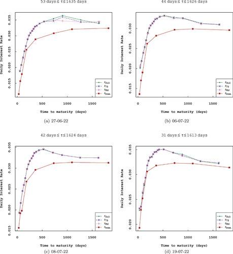
Figure 2. Estimated option-implied dividend yields obtained via the three estimation techniques (OLS, TS, and RM) across different maturities.

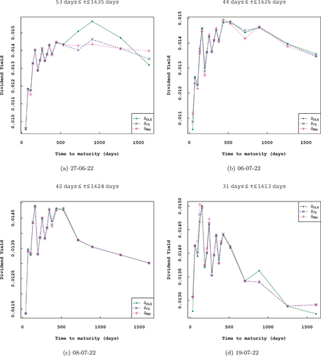
Figure 3. Comparison of estimated annualized option-implied dividend yields obtained via the three estimation techniques (OLS, TS, and RM) across different maturities with historical S&P 500 index yield.

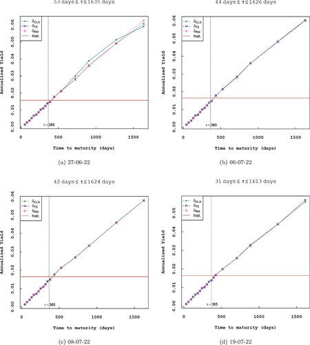
Table 5. The US. Daily treasury yield curve rates (%) between 27 June 2022 and 19 July 2022

	Maturity
Date	1 Mo	2 Mo	3 Mo	6 Mo	1 Yr	2 Yr	3 Yr	5 Yr	7 Yr	10 Yr	20 Yr	30 Yr
27-06-22	1.16	1.57	1.79	2.56	2.89	3.08	3.21	3.24	3.27	3.20	3.56	3.31
28-06-22	1.12	1.59	1.79	2.55	2.88	3.10	3.21	3.25	3.27	3.20	3.55	3.30
29-06-22	1.12	1.53	1.78	2.55	2.88	3.06	3.13	3.15	3.17	3.10	3.46	3.22
30-06-22	1.28	1.68	1.72	2.51	2.80	2.92	2.99	3.01	3.04	2.98	3.38	3.14
01-07-22	1.27	1.68	1.73	2.52	2.79	2.84	2.85	2.88	2.92	2.88	3.35	3.11
05-07-22	1.33	1.71	1.90	2.59	2.77	2.82	2.82	2.82	2.87	2.82	3.31	3.05
06-07-22	1.36	1.70	1.90	2.62	2.82	2.97	2.99	2.96	2.99	2.93	3.42	3.14
07-07-22	1.55	1.90	1.95	2.64	2.87	3.03	3.05	3.05	3.07	3.01	3.45	3.20
08-07-22	1.57	1.92	1.98	2.68	2.96	3.12	3.14	3.13	3.16	3.09	3.53	3.27
11-07-22	1.58	1.95	2.18	2.79	2.97	3.07	3.09	3.05	3.06	2.99	3.43	3.18
12-07-22	1.63	2.01	2.22	2.78	3.07	3.03	3.07	3.01	3.01	2.96	3.37	3.13
13-07-22	1.78	2.20	2.39	2.96	3.21	3.13	3.14	3.02	3.00	2.91	3.35	3.08
14-07-22	1.99	2.32	2.40	2.93	3.16	3.15	3.16	3.06	3.05	2.96	3.36	3.11
15-07-22	1.98	2.26	2.37	2.94	3.12	3.13	3.14	3.05	3.03	2.93	3.34	3.10
18-07-22	1.96	2.28	2.50	3.02	3.13	3.15	3.15	3.06	3.05	2.96	3.39	3.14
19-07-22	1.93	2.29	2.52	3.06	3.18	3.23	3.22	3.14	3.11	3.01	3.42	3.17

The option-implied risk-free interest rates obtained—via the three approaches earlier described—all yielded rates that were consistently higher than the treasury yield rates consistent with findings in past literature, see Golez and Jackwerth (2022) and van Binsbergen et al. (2022). For a detailed discussion on this convenience yield—the spread between the implied rates and treasury yields—readers are referred to van Binsbergen et al. (2022).

In the dividend yield estimation, the annualized implied dividend yields increase with time to maturity, see Figure 3.

From Figures 1, 2, and Figure 3, and by the results presented in Tables 1–4, the robustness of the repeated median is seen to be more pronounced even for heteroscedastic data compared to the OLS estimator.

6. Conclusion

In this article, a simple no-arbitrage methodology allowing for the simultaneous estimation of option-implied interest rates and dividend yields via a robust estimation method has been proposed. The estimators for the slope and intercept are derived from first principles via the no-arbitrage relationship, clearly demonstrating the link between the sloped asset position with the intercept and the box spread with the slope. Using market options data, robust forward-looking model-free estimates of the interest rate and dividend yield are obtained, with the robustness of the repeated median estimator being more pronounced even for heteroscedastic data. The characteristics of the option-implied risk-free interest rates and dividend information are consistent with findings in past literature, such as Golez and Jackwerth (2022), van Binsbergen et al. (2022), and Desmettre et al. (2017). Finally, these results point to a more informative approach in extracting other relevant information content from the market prices of options. The extent to which these option-implied rates and yields impact and compare with other “traditional” approaches whilst extracting other information from market prices of options is subject of future work.

Acknowledgments

The authors thank the Editor and the anonymous referees for their helpful comments and suggestions which helped improve an earlier version of this paper.

Disclosure statement

No potential conflict of interest was reported by the author(s).

Notes

1. Assuming that ex-dividend dates and the associated dividends are known with certainty for each of the stocks in the index.

2. The long call with strike $K_1$ has payoff $S_T-K_1$ and the short call with strike $K_2$ has payoff $K_2-S_T$. The total payoff is thus, $K_2-K_1$.

3. The long put with strike $K_2$ has payoff $K_2-S_T$ and the short put with strike $K_1$ has payoff $S_T-K_1$. The total payoff is again, $K_2-K_1$.

4. Although employing American options but correcting for the possibility of early exercise.

5. Golez and Jackwerth (2022) considered a slightly different regression: $S_t+P_i-C_i=Q_{t,T}+\beta K_i+{\xi }_i$

6. We only consider the direct estimation approach (as in (31)). Other intercept estimators exist that rely on the Theil–Sen slope estimate, see, for example, Dietz (1987). A common approach is often ${\hat{\alpha }}_{TS2}=\mathrm{m}\mathrm{e}\mathrm{d}\mathrm{i}\mathrm{a}\mathrm{n}\mathrm{o}\mathrm{f}[y_i-{\hat{\beta }}_{TS}{x}_i],\mathrm{f}\mathrm{o}\mathrm{r}i=1,2,\dots ,n$, where, $y_i=P_i-C_i$ and $x_i=K_i$.

7. Options expiring on the third Friday of each month.

8. These dates were picked at random.

9. For these options, unreasonable estimates (negative values) are obtained. In addition, treasury yield rates are not available for maturities less than 30 days. Hence, for comparative purposes, we chose to exclude the said options.

References

- Brenner, M., & Galai, D. (1986). Implied interest rates. The Journal of Business, 59(3), 493–20. https://doi.org/10.1086/296349
- Desmettre, S., Grün, S., & Seifried, F. T. (2017). Estimating discrete dividends by no-arbitrage. Quantitative Finance, 17(2), 261–274. https://doi.org/10.1080/14697688.2016.1176239
- Dietz, E. J. (1987). A comparison of robust estimators in simple linear regression. Communications in Statistics - Simulation & Computation, 16(4), 1209–1227. https://doi.org/10.1080/03610918708812645
- Geck, U. & Kaserer, C. (2021). Extracting convenience yield free short-term interest rates from equity derivatives (March 17, 2021). Available at SSRN: https://ssrn.com/abstract=3819767 or http://dx.doi.org/10.2139/ssrn.3819767.
- Golez, B. (2014). Expected returns and dividend growth rates implied by derivative markets. The Review of Financial Studies, 27(3), 790–822. https://doi.org/10.1093/rfs/hht131
- Golez, B. & Jackwerth, J. C. (2022). Holding period effects in dividend strip returns (June 9, 2022).
- Hull, J. C. (2018). Options, futures, and other derivatives (10th ed.). Pearson.
- Naranjo, L. (2009). Implied interest rates in a market with frictions. Working Paper,
- Ronn, A. G., & Ronn, E. I. (1989). The box spread arbitrage conditions: Theory, tests, and investment strategies. The Review of Financial Studies, 2(1), 91–108. https://doi.org/10.1093/rfs/2.1.91
- Sen, P. K. (1968). Estimates of the regression coefficient based on Kendall’s Tau. Journal of the American Statistical Association, 63(324), 1379–1389. https://doi.org/10.1080/01621459.1968.10480934
- Siegel, A. F. (1982). Robust regression using repeated medians. Biometrika, 69(1), 242–244. https://doi.org/10.1093/biomet/69.1.242
- Söderbäck, P., Blomvall, J., & Singull, M. (2022). Improved dividend estimation from intraday quotes. Entropy, 24(1), 95. https://doi.org/10.3390/e24010095
- Stoll, H. R. (1969). The relationship between put and call option prices. The Journal of Finance, 24(5), 801–824. https://doi.org/10.1111/j.1540-6261.1969.tb01694.x
- van Binsbergen, J., Brandt, M., & Koijen, R. (2012). On the timing and pricing of dividends. American Economic Review, 102(4), 1596–1618. https://doi.org/10.1257/aer.102.4.1596
- van Binsbergen, J. H., Diamond, W. F., & Grotteria, M. (2022). Risk-free interest rates. Journal of Financial Economics, 143(1), 1–29. https://doi.org/10.1016/j.jfineco.2021.06.012