Financial development and growth: Evidence from Bayesian Modelling

Abstract

This paper examines the nexus between financial development and economic growth in Ghana between 1970 and 2020. The study adopted the Bayesian Model Averaging (BMA) techniques to address issues of model uncertainty due to many potential explanatory variables that could influence growth. The study revealed that credit to the private sector, gross domestic savings, inflation rate, labour force participation, current account balance and population growth as key promoters of growth. Therefore, there is the need to address cost of doing business and promote increased credit delivery to the private sector. The direct association between financial development and growth indicates the need for policy makers to implement measures such as provision of legal environment for efficient allocation of credit to the private sector and provide the environment for the establishment of more financial institutions to enhance the growth of the financial sector.

Keywords:

• BMA
• Economic Growth
• Financial Development and Ghana

JEL Classification:

• C3
• G2
• G28

1. Introduction

Economic growth remains a central focus in economic policy formulation for centuries due to the significant roles it plays in describing the health and direction of an economy. One of the significant drivers of economic growth identified in the extant literature is financial development (Čihák et al., 2012 & Chowdhury, 2016). To deepen the role of the financial sector in the development of the Ghanaian economy, the government of Ghana established the Ghana Commercial Bank (GCB) in 1953 and the Bank of Ghana (BoG) after independence to play a critical role in the advancement of the economy. Though other financial institutions were established after GCB and BoG, the sector was not able to effectively promote funds to the priority areas of the economy, and by 1983, the financial sector was largely characterised by financial shallowing and repression as this sector has a strong link with growth (McKinnon, 1973; Shaw, 1973).

To address the challenges in the financial sector, the government of Ghana in 1983 implemented the Financial Sector Adjustment Programme (FINSAP) with a key policy thrust being financial sector liberalisation. The liberalisation of the financial sector has resulted in a considerable increase in the number of financial institutions.

To establish the role of the financial sector in Ghana’s economic development, a plethora of empirical studies used various indicators selected from the stock market and banking sectors as proxies for measuring financial development (Amoah et al., 2021). A vast majority of the studies selected private sector credit to GDP, broad money to GDP, narrow money to broad money, currency to broad money, currency to GDP, total domestic credit to GDP, stock market capitalisation to GDP, among others. This makes the findings from the finance–growth nexus studies mixed and sensitive depending on the proxy used.

On the nexus between growth and financial development, Uddin et al. (2013) used various indicators such as domestic credit provided by banking sector as a percentage of GDP, domestic credit to private sector as a percentage of GDP, money plus quasi money (M2) as a ratio of money (M1) and with the help of principal component method (PCM) constructed financial index. Using a Cobb–Douglas production augmented function by incorporating financial development and simulation based on ARDL bounds testing and Gregory and Hansen’s structural break cointegration approaches, the paper found a positive relationship between the two variables of interest. In addition, Kar et al. (2011) used a bootstrap panel Granger causality analysis to look at the finance-growth relationship in Asian nations from 1980 to 2007. The study found a positive association between financial development and growth using time series analysis. Zhang et al. (2012) used growth in money supply as proxy for financial development and discovered a positive relationship between financial development and economic growth in their study using GMM estimators for dynamic panel data, ARCH estimate, Granger regression and ECM model, respectively. Furthermore, Khan et al. (2005) used total bank deposit liabilities to nominal GDP and deposit rate as indicators for financial depth and employed an autoregressive distributed lag approach and found that financial depth exerted a positive impact on economic growth in the long run but the relationship was insignificant in the short run, but also had impact on growth in both the long and the short run. Allen and Ndikumana (1998) examined the role of financial intermediaries in fostering economic growth in Southern Africa using a variety of financial development indicators such as domestic credit to the private sector, stock market capitalisation as well as public and private bond market capitalisation using a growth equation; the findings revealed that there is a link between financial development and economic growth.

The review of the empirical literature on the relationship has shown two major challenges. Firstly, some of these studies are mainly based on the bi-variate causality test. Yet, it is now clear that a bi-variate causality test may be very unreliable, as the introduction of a third important variable can change both the inference and the magnitude of the estimates (Caporale & Pittis, 1997; Caporale et al., 2004; Odhiambo, 2008). Secondly, in the light of the complexity of measuring financial development due to the selection of multiple parameters, the evidence from the literature indicates that the effect of financial development on economic growth is contingent on the measure of financial development indicator employed (Adu, Marbuah, & Mensah, 2013). Clearly, it is also impossible for previous studies to determine the magnitude of the impact of each indicator of financial development on growth.

Again, evidence from various empirical works like Amoah et al. (2021), Agrawal (2000) and Uddin et al. (2013) among others has revealed that the relationship between financial development and growth would depend on how financial development is measured and the model adopted. In most of these empirical studies, variables to be included in the model are limited. With a limited number of observations, it is inefficient or even infeasible to do inference on a single linear model that includes several variables. In addition, in a canonical regression, problem arises when there are many potential explanatory variables which make it difficult to determine which variables should be included in the model and how important they are in explaining the dependent variable. These issues raise much concern about the uncertainty of the economic model adopted in the previous studies.

Therefore, to address these problems in the literature, the study adopted the Bayesian Model Averaging to deal with the issue of model uncertainty and large size of regressors in determining the link and the magnitude of each indicator’s contribution to growth. This is because the BMA approach tackles the problem by estimating models for all possible combinations of the explanatory variables and constructing a weighted average over all of them (Raftery et al., 1997; Fernandez et al., 2001).

To the best of our knowledge, there is no existing literature that uses BMA to estimate the effect and magnitude of financial development on economic growth in Ghana. Therefore, the contribution of this paper is to fill the gap in literature by dealing with the issue of model uncertainty and large size regressors. Finally, the findings from this study will enable policy makers to prioritise the indicators in the financial sector to promote rapid growth.

The subsequent portions of the paper are organised as follows: The next section outlines overview and trends of financial development and growth, theoretical underpinning and model specification. The subsequent section presents and discusses the empirical analysis, and the final section summarises the results and policy recommendations.

2. Overview and trends of financial development and economic growth in Ghana

In the late 1970s, the Ghanaian economy experienced a rapid economic deterioration in the form of negative economic growth, high levels of inflation, fall in domestic savings and investment, deficit balance of payment, high unemployment rate and negative macroeconomic indicators among others (Data from WDI,2020).

Before the introduction of the financial reforms, the economy was characterised by both closed and open policies during the period from independence. During the financial repressive regime, direct control measures were adopted in the financial sector with interest rates and exchange rate determined by the central government. Monetary policy was carried out by the Central Bank through the implementation of instruments such as the required reserve ratio, special deposit, credit control and moral suasion. This situation made it highly impossible for the commercial banks to create credit for the private sector for productive investment and hence economic growth (World Bank, 1981).

Figure 1 shows the trend of GDP growth rate vis-a-vis the broad money and the monetary sector credit to the private sector as percentages of GDP, respectively.

Figure 1. Growth, broad money and credit to the private sector trends, 1970–2020.

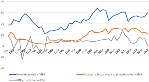
During the late 1970s, most, if not all, economic indicators worsened with average growth rate of −0.53% from 1971 to 1982 with the worse growth rate of −12.43% recorded in 1975 and the highest growth rate of 8.47% recorded in 1978. This deteriorating performance could be attributed to a state-controlled economy, which was characterised by stringent import controls, domestic price controls and fixed exchange rates, to contain inflation.

However, in the early stages of the reforms, the economic growth performance of the economy remained highly volatile. During the period 2005 to 2007, the economy was growing at an average rate of 5.5% and this was largely attributed to the power rationing and energy shortages resulting from the low water level in the Akosombo Dam. In 2011, the economy grew at a rate of 14.04%, the highest Ghana had recorded since 1970–2020. This was attributed to offshore oil production which started in the country in late 2010. However, this growth trend was not sustained; it fell to 9.3 % in 2012. This fall in the growth rate was due to the uncertainty of investors to invest in the economy (during this particular period as the country was involved in the elections). The economy of Ghana expanded 3.6% year-on-year in the third quarter of 2015, easing from a 3.9% growth in the previous period and 12.2% a year earlier.

However, World Bank (2012) report had classified Ghana among the best performing countries in Sub-Saharan Africa in terms of financial sector reform policies. The average financial depth in Ghana has shown a significant improvement since 2005, but the growth rate of the country during the same period shows some level of volatility.

2.1. Review of related works on financial development and economic growth

The importance of financial sector to growth and development of a nation has been an area of concern to researchers, governments and the players in the financial sector. The directional relationship between financial development and economic growth has been a long debate for centuries. Empirical works on this relationship have produced mixed results largely due to the methodologies used and the indicators used as proxies for financial development.

On the role of finance to development, there are two schools of thoughts. The first is the supply-leading finance hypothesis proponents who view the role of finance as key in economic growth (Gerschenkron, 1962; Patrick, 1966; Schumpeter, 1912). This school of thought views the creation of financial institutions and supply of other financial assets in advance before demand by businesses to promote growth as it may ensure re-allocation of resources from older, less productive sectors to newer, more productive sectors. Schumpeter (1912) emphasised the importance of financial intermediation in boosting productivity and stimulating economic growth. He was of the view that financial intermediaries play a critical role in economic transformation by mobilising savings or funds, evaluating and selecting projects, managing risk, monitoring entrepreneurs and facilitating transactions. By doing so, Schumpeter believed that a portion of savings would be invested in projects, and that an increase in investment would have a direct positive effect on economic growth. In addition, examples finance theorists also believe that the amount and make-up of financial variables directly increases savings in the form of financial assets, which in turn spurs capital formation and, ultimately, economic growth.

Allen et al. (2012) also conducted empirical research on the claim made by Schumpeter (1911) on the positive impact of financial development to growth but only ended up forming the same conclusion that financial development drives economic growth. Specifically, Allen et al. (2012) discovered a positive and significant impact of Equity Bank, a leading private commercial bank, on financial access, particularly for underprivileged households, using extensive country and firm-level data sets. According to the study, this was due to Equity Bank’s business model, which enabled the bank to generate sustainable profits by providing financial services to population segments typically ignored by traditional commercial banks.

On the second school, financial repression theorists led by McKinnon (1973) and Shaw (1973), financial liberalisation would result in positive real rates on cash balances which would serve as a means of fostering economic expansion. The McKinnon-Shaw hypothesis also provided support to supply-leading argument on the need to channel funds from surplus to deficit units for investment, resulting in economic growth. By so doing, McKinnon (1973) proposed a complementarity relationship between the accumulation of financial assets and the accumulation of physical capital in developing countries.

However, Patrick (1966) further argued that the causal relationship between financial development and economic growth varies depending on the stage of development. He contends that during the early stages of development, the supply-leading pattern predominates. As financial and economic development progresses, the supply-leading characteristics of financial development gradually fade, and demand-following financial development eventually takes over.

Using exchange rate as a proxy for financial development, Ehigiamusoe and Lean (2019) examined the nexus between exchange rate and its volatility on growth. Using panel data from West African countries, the findings established long run effect on growth, but this impact reduces as there is a volatility in the exchange rate. It further indicates that the impact of the exchange rate on growth depends on the level of volatility. The study therefore recommends a reduction and stability in exchange rate to have its full impact on growth.

In the Ghanaian context, Ibrahim and Alagidede (2019) investigated the dynamic asymmetric effects of financial development on growth in Ghana from 1980 to 2016. The study used a nonlinear autoregressive distributed lag approach to cointegration. The study’s findings revealed the existence of a long-run asymmetric relationship, with both positive and negative shocks to financial development having distinct long-run and short-run effects on economic growth. This demonstrated that the growth effects of financial development are premised on the nature of the financial sector’s shock.

On the contrary, Lewis (1954) introduced a time dimension into the debate, arguing that initially economic growth facilitates the formation of financial markets, and that over time, a matured financial market promotes economic growth, implying a bidirectional relationship between financial development and economic growth.

Samargandi et al. (2015) used a panel of 52 middle-income countries over the period of 1980–2008 to revisit the relationship between financial development and economic growth. The study employed the pooled mean group estimations in a dynamic heterogeneous panel setting. The findings indicated that there existed an inverted U-shaped relationship between finance and growth in the long run. However, in the short run, the relationship was insignificant, suggesting that too much finance can exert a negative influence on growth in middle-income countries. Also, the study confirmed the existence of a non-monotonic effect of financial development on growth by estimating a threshold model.

In estimation, the selection of appropriate variables arises when there are many potential explanatory variables which make it difficult to determine which variables to include in the model and how important they are in explaining the dependent variable. Secondly, with a limited number of observations, it is inefficient or even not feasible to make inferences on a single linear model that includes several variables. One of the key restrictions about models employed by previous studies is that they all used single equation models for the empirical test of the growth-finance nexus with the basic assumption that financial factors are exogenous determinants of economic growth, thus suggesting a unidirectional causality from finance to growth. To address the issues of model uncertainty due to many potential explanatory variables that could influence the nexus between growth and finance, the paper adopted the BMA techniques. This method addresses the issues by estimating models for all possible combinations of the explanatory variables and constructing a weighted average over all of them and models with high likelihood functions are obtained by averaging across a large set of models and selecting variables that are relevant with high posterior probability to enable the selection of parsimonious and accurate predictors.

3. Methodology

3.1. Model specification

Selecting appropriate variables when there are many potential explanatory variables makes it difficult to determine which variables to include in the estimation and how important these variables will be in explaining the dependent variable. Secondly, with the issue of limited number of observations in most studies which are not feasible to make inferences on a single linear model that includes several variables, to address the issues of model uncertainty due to many potential explanatory variables that could influence the nexus between growth and finance, the study adopted the BMA techniques. The rationale of the BMA approach is that for a given linear model with many explanatory variables (k); there are 2^k possible models that can be obtained by the selection of explanatory variables. Appropriate models with high likelihood of solving model uncertainty are obtained by averaging across the large set of models and selecting variables that are relevant to the data generating process for a given set of parameters and model priors used (Fernandez, Ley & Steel, 2001; Raftery et al., 1997). Parameter and model sampling in the context of the BMA approach are conducted with the aid of the Markov Chain Monte Carlo Model Composition (MC³). The MC³ method is used to indicate which model should be considered in computing the sums of posterior model and parameter probabilities by identifying the model with high posterior probability.

Given a linear regression model with ${\beta }_i$parameters and $i=0,1,2,...,k$, with $k$explanatory variables $x_1,x_2,x_3,...,x_k$, the general form of the regression is

(1) $y=\beta 0+\sum _{i=1}^k{\beta }_i{x}_i+\epsilon$(1)

Given $k$ explanatory variables, there is a possibility of $2^k$ models to be obtained with the different combination of explanatory variables. The posterior distribution of the parameters${\beta }_i$, given the data D, is an average of the posterior distribution of parameters under each model with weights given by the posterior model probabilities expressed as:

(2) $P({\beta }_i/D)=\sum _{j=1,{\beta }_i\in Mj}^{2^k}P({\beta }_i/M_j)P(M_j/D)$(2)

The posterior model probability $P(M_j/D)$ is given by:

(3) $P(M_j/D)=\frac{l_D(M_j)P(M_j)}{\sum _{h=1}^{2^k}{l}_D(M_h)P(M_h)}$(3)

where $l_D(M_j)$ is the marginal likelihood of the model $M_j$ which is expressed as

$l_D(M_j)=\int p(D/{\beta }_i,M_j)p({\beta }_i)p({\beta }_i/M_j)d{\beta }_i$

where $P(D/{\beta }_i,M_j)$represents the sampling model corresponding to Equation 1. $P(\beta i/Mj)$ is a prior probability distribution assigned to the parameters of model $M_j$, and $P({\beta }_i)$is the improper non- informative prior for the parameters that are common to all models. The Zellner’s g-prior is the preferred choice of prior structure for the regression parameters in most BMA applications. The common improper non-informative g-prior structure for $P(\beta i)$ is often expressed as:

(4) $P(\beta i)\propto {\sigma }^{-1}$(4)

where $\sigma$ is a scale parameter that represents the standard error of the regression represented in Equation 1(1) $y=\beta 0+\sum _{i=1}^k{\beta }_i{x}_i+\epsilon$(1) .

Nonetheless, Fernandez et al. (2001) proposed a g-prior for $P(\beta i/Mj)$and suggest that a uniform a prior be represented as$g=1/max\left\{n,k^2\right\}$. The authors show that such a g-prior leads to reasonable results.

With regard to model probability prior$P(M_j)$, the proposed prior distribution in the literature of BMA refers to uniform distribution prior expressed as:

(5) $P(M_j)=p_{j,}j=1,2...,2^k\mathrm{w}\mathrm{i}\mathrm{t}\mathrm{h}\sum _{j=1}^{2^k}{p}_j=1$(5)

Following Leamer (1978), the estimated posterior means and standard deviations of $\beta i$, $\hat{\beta }$, are constructed as:

(6) $E(\hat{\beta }/D)=\sum _{j=1}^{2^k}\hat{\beta }P(M_j/D)$(6)

(7) $V(\widehat{\beta }/D)=\sum j={12}^k(Var(\widehat{\beta }/D,Mj)+\stackrel{\beta }{}2)P(M_j/D)-E{(B/D)}^2$(7)

Different model priors are used to obtain posterior parameter and model results. This is essential to assure the robustness and consistency of our results.

3.2. Data, empirical results and discussion

Appendix Table A1 presents variables assumed to be candidates of explanatory variables of economic variables in Ghana based on literature and economic development theories. There are, a total of, 26 variables used in the model estimation, including the annual growth in GDP as the dependent variable and 25 potential explanatory variables.

Choosing an appropriate measure of financial development is crucial to analysing the relationship between financial development and economic growth. Construction of financial development indicators is an extremely difficult task because of the diversity of financial services catered for in the financial system (Ang & McKibbin, 2005). Several indicators of financial depth have been used in the empirical literature as a proxy for development of the financial sector. These are domestic credit to the private sector, stock market capitalisation, total value of stock trade, turnover ratio, gross domestic savings and the ratio of broad money to GDP. Most empirical studies in this area use one indicator at a time to determine the link. However, to solve the problem of uncertainty related to the use of a single indicator, all the indicators of financial development are included in the BMA estimation.

The ratio of broad money (M2) to GDP is also considered as standard measure of financial development (World Bank, 1981). However, this ratio measures the extent of monetisation rather than financial development (Khan & Qayyum, 2006). In most developing countries, a higher ratio of money to GDP may not necessarily reflect increased financial depth, as money is used as a store of value in the absence of other more attractive alternatives (Khan & Senhadji, 2003).

The second measure of financial development is the ratio of domestic credit to the private sector to GDP. This ratio excludes the public sector and therefore reflects more efficient resource allocation in the economy, since the private sector can utilise funds in a more efficient and productive manner than the public sector. The next ratio, private sector credit to domestic credit shows the share of credit to the private sector in total domestic credit and measures the extent to which the banking system channel funds to the private sector to facilitate investment and growth.

Stock market capitalisation is the ratio of the value of listed domestic shares to GDP. Total Value Traded, as an indicator to measure market activity, is the ratio of the value of domestic shares traded on domestic exchanges to GDP and can be used to gauge market liquidity on an economy-wide basis. The turnover ratio (TOR) is the ratio of the value of domestic share transactions on domestic exchanges to the total value of listed domestic shares. A high value of the turnover ratio will indicate a more liquid (and potentially more efficient) equity market.

Other explanatory variables used in the model include the current account balance per GDP, inflation, literacy level measured as the total secondary school enrolment, annual population growth, total crop production per GDP, population density, capital formation per GDP total domestic debt stock of the economy per GDP, total external debt stock of the economy per GDP, taxes of profit, custom tax, labour force participation rate and gross infrastructure development which is measured as a proxy with the number of telephone line per 100 people. Yearly data ranging from 1970 to 2 020 are collected from the World Bank Development Index (WDI, 2021) and International Monetary Fund (IMF) statistics.

To ensure that there is no issue of possible multicollinearity in the estimation, a correlation matrix was performed (Appendix Table A2) and the cross-correlation values revealed the absence of perfect collinearity. In addition, to ascertain that all variables are stationary and that there is no possibility of cointegration between them, the paper applies the Dickey–Fuller Generalised Least Square (DF-GLS) test of unit root as proposed by Elliott, Rothenberg, and Stock (1996). This test has significantly greater power than the previous versions of the augmented Dickey—Fuller (ADF) test.

4. Empirical results and discussion

Appendix Table A3 presents the descriptive statistics of the variables used in the paper. The result shows that on average from 1970 to 2020, the average GDP growth (annual %) is 3.9% with a minimum of −12.4% and a maximum of 14.0%. Besides, the average broad money growth as a percentage of GDP is about 34.8% with the lowest being 10.0% and a maximum percent of 68.5%. In addition, average rate of inflation doing the period under consideration was 29.1% with the country debt accounting for an average of 54.2%. The total debt servicing as a percentage of GDP doing the period amounted to an average of 3.9% with import and export to GDP accounting for 32.6% and 24.4%, respectively.

The results of the BMA analysis represented in Table 1 are obtained with the model aprior set to $2^k$ (where $k=25,$ is the number of explanatory variables included in the model). The prior probability of the regression coefficients is constructed by using the Bayesian Information Criterion (BIC) for all the models with the assumption that the coefficients of the various independent variables are distributed with zero mean and a variance that follows the Zellner’s g-prior structures. Moreover, the $M{C}^3$ sampling employed is based on taking 1000 000 draws, from which 100 000 draws are discarded as burn-ins replications to obtain model and coefficient posteriors. The paper follows Raftery (1995) by suggesting that for a variable to be considered as an effective driver of economic growth its posterior inclusion probability must be at least 20%. Since this criterion, the following regressors are identified; domestic credit to the private sector, gross domestic savings, inflation, population growth, labour force participating rate and current account balance among others.

Table 1. Bayesian model averaging results

Codes	PIP	Post Mean	Post SD
DCP	1.00	0.03	0.00
INFL	0.70	−0.02	0.02
GDS	0.46	0.05	0.07
POPGR	0.46	0.00	0.00
LFP	0.42	−0.01	0.01
CUCAC	0.26	0.73	1.75
LR	0.18	−0.32	1.00
INFRA	0.17	0.02	0.07
DR	0.17	0.00	0.03
CROP	0.16	0.00	0.02
TOS	0.16	0.00	0.04
PERCA	0.16	0.01	0.03
BM	0.15	−0.01	0.08
LIT	0.14	6.93	60.82
DEBT	0.14	0.00	0.01
IMP	0.14	0.01	0.03
ATAX	0.14	0.00	0.01
GDPPER	0.13	−0.31	1.95
TAXPR	0.12	0.00	0.02
DEBTSER	0.12	0.00	0.05
TST	0.12	−0.02	0.37
MARCA	0.11	0.00	0.01
NDEPO	0.11	0.01	0.38
CAF	0.11	0.00	0.02
EXP	0.10	0.00	0.02

Source: Computed from, WDI (2022)

From the results on Table 1, the link between financial development and economic growth is given by the Posterior Inclusion Probabilities (PIP) reported in the first column. The PIP shows the percentage of the model space wherein a covariate is included. The last two columns contain the posterior means and standard deviation for each regression parameters, averaged across models.

Based on the level of significance (at least 10% level of significance) of covariates averaged across the model, the results of the BMA analysis reported in Table 1 show the importance of financial development to economic growth. From the results in Table 1, domestic credit to the private sector is found to have a positive impact on growth with a PIP of 100%. This means that as credit to the private sector increases, the performance of the economy would also improve. This is because as more credits become available to the private sector at a cheaper rate of interest, it encourages the businesses or the firms to borrow more which will facilitate the growth of business or increase production and economic activities that will result in growth. In addition, the increases in savings because of the credit available to the private sector will propel investment as identified in the work of McKinnon (1973) and Shaw (1973). However, the finding from this study is in contradiction to the study of Ahmad and Malik (2009) and Esso (2009) who found a negative but significant relationship when private sector credit and growth.

Gross domestic savings in the economy have the expected positive sign and exert statistically significant effects on growth with PIP of 46.4%. This is because savings is very critical to growth of any economy due to it relation to investment. A higher savings rate will lead to an increase in real income and a larger steady-state capital stock and higher output levels. A larger savings rate, according to certain recent growth theories, may boost the rate of economic growth indefinitely. This relationship is in conformity with the supply leading view of the relationship between financial development and economic growth in accordance with the prediction by the McKinnon–Shaw hypothesis. It is also in conformity with the finding of Kiran et al. (2009), Allen and Ndikumana (1998), and Odhiambo (2008) but contradicts the findings of Quartey and Prah (2008) for Ghana and Ahmad and Malik (2009) for Sierra Leone.

From the results presented in Table 1, in addition to financial development indicators, other variables such as inflation rates, labour participation rate, crop production, current account balance, population growth and infrastructure development are also found to have a link with economic growth in Ghana. The negative sign of the inflation rate indicates the damaging effect that inflation can cause to economic growth. The inflation targeting policy as adopted by the Ghanaian monetary authority should be strictly adhered to. A high level of the labour participation rate is found to hamper economic growth in Ghana. This reality is commensurate with the fact that the public sector remains the single most important source of employment for job seekers in Africa and Ghana in particular. While this situation is not peculiar to Africa or Ghana, the poor development of the private sector forces government to absorb job seekers, sometimes for political reasons, causing a diminishing return to labour hence detrimental to growth.

The population growth of the country has an inverse relationship with growth with a PIP of 46%. This implies that the rate of population growth plays a critical role in determining the rate of economic progress. This is because a rapid population exacerbates the difficult choice between higher consumption in the present and the investment needed to bring higher consumption in the future. As populations grow, larger investments are needed just to maintain current capital/person. In addition, the rapid population growth also tends to reduce arable land available for economic activities to increase the output of the country but rather increasing sanitation and pollution problems which hinders economic progress of the country. This inverse relationship finding is in conformity with the findings of Easterlin, R., (1967), who studied the effects of population growth on the economic development of developing Countries.

Total crop production contributes positively to the Ghana’s economic growth. There are several reasons supporting this finding. Firstly, the increase in crop production will mean lower import of consumption goods and a sound current account balance. This situation implies that the focus is put on importing capital rather than consumption goods. Secondly, the increase in total crop production helps to stabilise the general price level leading to low inflation and this will boost investors’ confidence level and, thus, economic growth. This finding is in conformity with Rask and Rask (2011) who found a positive link between food production and economic development in developing economies.

The improvement of the current account balance has a positive effect on economic growth in Ghana. As stated earlier, a sound current account provides countries such as Ghana with the financial resources to finance import, especially the import of capital goods, which is necessary for economic growth. Moreover, a sound current account alludes to the importance of export revenues and trade openness for Ghana. The literature abounds on the positive effect of trade openness on economic growth, through its effect on the current account (Jiang, 2011; Lloyd & MacLaren, 2000).

The findings of this paper allude to the importance of infrastructural development (for which the proxy of the number of telephone line per total population was used), on economic growth in Ghana. A few authors refer to the importance of infrastructural development on economic growth, especially in the context of developing and emerging economies (Alfonso, 2007; Kohei & Ken, 2013; Pradhan Rudra & Bagchi Tapan, 2013).

To gain insight into the degree of uncertainty that single model estimation could provide when assessing the nexus between financial development and economic growth, the results reported in Table 2 are compared with those in Table 1. Table 2 provides the results of the first five best single models, classified by the magnitude of the model posterior probability calculated from models visited by the $M{C}^3$ algorithm. The results reported in Table 2 indicate how misleading could be any policy formulation that relies on the single-model estimation. For example, Model 3, in Table 2, indicates the domestic credit to the private sector and inflation rate are importance explanatory variables. However, this model has the posterior model probability of 0.035(3.5%), which means that policymakers who base their recommendation on this estimation will be more than 96.5% sure it is not the correct model.

Table 2. Posterior means of the best five models

	Model 1	Model 2	Model 3	Model 4	Model 5
Inter	3.97045	4.80714	3.98963	3.99432	3.99153
BM	.	.	.	.	.
ATAX	.	.	.	.	.
PERCA	.	.	.	.	.
POPGR	.	.	.	.	.
IMP	.	.	.	.	.
GDPER	.	.	.	.	.
DEBT	.	.	.	.	.
DEBTSER	.	.	.	.	.
DR	.	.	.	.	.
CROP	.	.	.	.	.
CAF	.	.	.	.	.
TAXPR	.	.	.	.	.
LFP	−0.01562	−0.01531	.	.	−0.01622
INFRA	.	.	.	.	.
LIT	.	.	.	.	.
DCP	0.03177	0.03212	0.03199	0.03222	0.03155
INFL	−0.03843	−0.03913	−0.03819	−0.03921	−0.03904
GDS	0.12495	0.13405	.	0.07881	0.12316
MARCA	.	.	.	.	.
NDEPO	.	.	.	.	.
LR	.	.	.	.	−1.8262
CUCAC	.	2.98157	.	.	.
TOS	.	.	.	.	.
Exp	.	.	.	.	.
TST	.	.	.	.	.
NVar	4	5	2	3	5
r2	0.933	0.936	0.919	0.924	0.935
post prob	0.094	0.045	0.035	0.028	0.028

Author’s computation (2022)

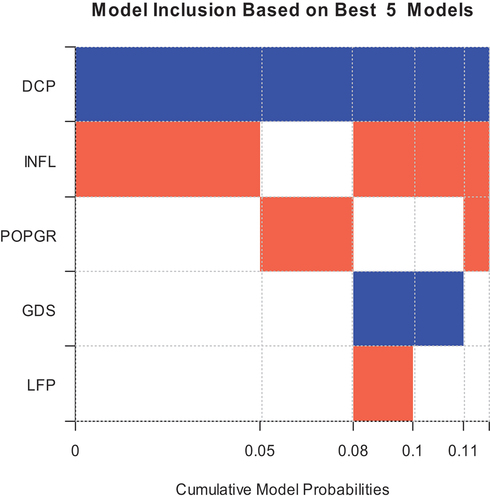
In addition, Figure 2 shows the cumulative model probabilities model inclusion based on the best five model for Ghana. The best model, with 79.3% posterior model probability, is the one that only includes domestic credit to the private sector. However, the second-best model includes the rate of inflation in addition and has a PMP of 7.5%. The third, fourth and the fifth include population growth, gross domestic savings and labour force participating rate with PMP of 3.6%, 2.9% and 2.7%, respectively. Details of the PMP and MCMC values and graphs are shown in Appendix Table A4 and Figure A1.

Figure 2. Cumulative model Probabilities.

To address the issue of overfitting and low shrinkage factor and test the sensitivity and robustness of our results, we re-estimated the BMA model by using different g-priors such as “flexible” (Liang & Jian-Zhou, 2006) as this adapt to the data. Using the 20% threshold of the posterior inclusion probability, the results reported in Tables A1, A5, A6 and A7 indicate variables such as domestic credit to the private sector, inflation rate, gross domestic savings, labour force participation, population growth and current account balance are key to economic growth. These results are consistent with those obtained when using a model “g-prior=UIP” prior, except for the infrastructure development whose PIP has now increase above the 20%. This finding gives an assurance that our results are robust and consistent with the change of coefficient priors.

5. Conclusion and policy recommendation

The main aim of this study was to address the issue of model uncertainty associated with previous studies in assessing the link between financial development and economic growth in Ghana by adopting the Bayesian model averaging. Credit to the private sector and gross domestic savings as a proxy for financial development are found to be highly significant with a high PIP and positively related to promoting growth as suggested by Kiran et al. (2009), Odhiambo (2008) and Khan and Qayyum (2006). Though the other financial development indicators are also important and have the expected signs, their PIPs are below the threshold of 20%.

In addition, growth in infrastructure investment, total crop production of the country and the current account balance play a key role in influencing growth positively. However, the labour force participation rate, inflation and population growth are found to influence economic growth negatively.

To promote growth through financial development, policies should be formulated to facilitate the establishment of financial institutions to increase credit delivery to the private sector.

Further government should provide the legal environment for efficient allocation of credit to the private sector through the adoption of reforms to strengthen creditors’ rights and enforce commercial contracts and establish incentive frameworks that will encourage savings and investment.

Government through supply side policies like tax holidays to domestic firms provide the enabling environment for businesses to improve their competitiveness in both domestic and export. Secondly, government through ministry of trade and industry should encourage consumption of made in Ghana products and reduce domestic consumption and spending on imports by using tight fiscal policy like higher taxes on imported goods, and these policies will result in improved current account balance that has a positive link with growth. However, any future research on this issue should consider the possibility of exploring the TVP-VAR model to cater for time variations.

Disclosure statement

No potential conflict of interest was reported by the author(s).

Additional information

Notes on contributors

Ferdinand Ahiakpor

Ferdinand Ahiakpor is currently a Professor in School of Economics, University of Cape Coast, Ghana with over 18 years working experience. Ferdinand teaches and supervises various courses and thesis at both undergraduate and graduate levels. As an economist, Ferdinand published several articles, policy briefs, technical papers and presented academic and policy papers at both national and international levels.

Ralph Nordjo

Ferdinand has several years of working experience both nationally and internationally. Ferdinand between 2018 and 2022 served as a short-term Consultant for the United Nations Economic Commission for Africa (UNECA), Macroeconomic Policy Division, with the responsibility of developing and training key stakeholders on E-Views-based Macroeconomic Model for selected African countries. Ferdinand graduated from University of Cape Coast where he obtained Ph.D. in Economics.

Samuel Erasmus Alnaa

My speciality though not limited covers Macroeconomic Modelling, Fiscal policies, Monetary Policies, Sovereign Risk Analysis Labour Market Analysis and Development Economics.

Appendices

Table A1. Model variables

Codes	Full names
Gr	GDP growth
Inf	Annual rate of inflation
Lit	Total secondary school enrollment
Perca	GDP per capita
Debt	Debt per GDP
debtser	Total debt servicing per GDP
Bm	Broad money growth
Popgr	Annual population growth
caf	Fixed capital formation
Infra	Telephone per 100 people
Popden	Population density
Taxpr	Tax on profit
atax	Average tax to GDP
Exp	Export per GDP
Dcp	Domestic credit to the private sector
Marca	Market capitalisation of listed companies
Dr	Deposit rate
Lr	Lending rate
Crop	Total agriculture production per GDP
Gds	Gross domestic savings
Ndepo	Total number of depositors with commercial banks
Tst	Total value of stock traded
ToS	Turnover in the stock market
Cucac	Current account balance per GDP

Source: Author’s Construct, (2022)

Table A2. Correlation matrix of variables

	gr	bm	atax	perca	popgr	imp	infra	debtser	debt	taxpr	cucac	dr	lfp	infl	dcp	ndepo	lr	crop	gds	exp	tst
gr	1
bm	−0.0212	1
atax	−0.0591	0.2148	1
perca	0.1082	0.0285	−0.0032	1
popgr	−0.1985	0.0818	0.0579	−0.099	1
imp	−0.333	0.1675	0.1108	−0.1042	0.1521	1
infra	0.0626	−0.0637	0.0096	0.014	−0.0301	−0.2133	1
debtser	−0.0538	0.0737	0.0755	0.1383	0.1373	0.2345	0.1223	1
debt	−0.1244	−0.0694	0.2561	0.1958	0.1704	−0.0627	0.2386	0.4489	1
taxpr	−0.0341	0.0666	0.1213	0.4511	−0.0764	−0.0119	−0.1088	0.2095	0.2594	1
cucac	0.1417	−0.3482	−0.3695	−0.1004	0.0109	−0.0258	−0.1321	0.0645	0.0292	0.0001	1
dr	0.1235	0.0532	0.1312	0.335	0.0376	−0.0964	0.4749	0.3503	0.5542	0.2714	−0.0966	1
lfp	−0.2123	−0.2156	0.0845	0.0215	0.178	−0.1591	−0.0569	0.1349	0.1614	0.159	−0.0106	0.0388	1
infl	−0.1153	0.0825	−0.0173	−0.1222	−0.0843	0.1541	−0.0453	−0.0235	0.0562	−0.0179	−0.063	−0.0108	−0.0211	1
dcp	0.947	−0.0549	−0.1288	0.082	−0.1704	−0.3726	0.009	−0.046	−0.1281	−0.0555	0.2914	0.0802	−0.1598	−0.131	1
ndepo	0.1293	−0.2503	−0.2242	0.1193	−0.0318	−0.0851	0.0036	0.085	−0.0034	0.0935	0.6963	−0.0775	0.0039	−0.0761	0.2864	1
lr	−0.1721	0.1345	−0.1416	−0.1054	−0.1517	−0.0126	−0.0085	−0.0825	−0.0692	−0.0479	−0.0992	−0.0925	−0.0803	−0.0548	−0.1471	−0.0984	1
crop	0.1103	0.2442	−0.1441	0.2977	−0.1023	−0.2009	0.0947	0.0968	0.2719	0.241	0.0624	0.3385	0.0671	0.0006	0.1585	0.0093	−0.0858	1
gds	0.1136	−0.0094	0.0811	0.2841	0.001	0.0482	−0.0453	−0.1112	−0.136	−0.0366	0.0083	0.1947	−0.0289	−0.3797	0.1325	−0.0176	0.0012	0.1182	1
exp	0.0341	0.1243	0.1401	0.0145	0.0365	−0.0127	0.2437	0.3583	0.6497	0.2528	−0.0366	0.7506	0.0279	0.1283	0.0209	−0.0704	−0.07	0.3456	0.0094	1
tst	0.0764	−0.0323	0.0406	0.0176	0.158	−0.0075	0.1883	0.074	−0.0515	−0.1106	−0.1554	0.079	−0.0495	−0.4279	0.0719	−0.0418	0.0015	−0.1383	0.4153	0.0744	1

Source: Author’s Construct, (2022)

Table A3. Descriptive statistics

Code	Mean	Std. Dev.	Min	Max
gr	3.9	4.5	−12.4	14.0
infl	29.1	27.6	3.0	122.9
bm	34.8	14.3	10.0	68.5
cucac	−4.9	3.7	−12.5	3.1
dcp	8.5	4.5	1.5	15.9
debt	54.2	32.4	16.5	139.4
Debtser	3.9	2.6	0.8	10.8
Exp	24.4	11.3	3.3	48.8
Imp	32.6	17.0	3.0	67.2
Lit	45.3	14.5	33.3	77.7
Lr	25.3	10.0	8.5	47.0
Exp	24.4	11.3	3.3	48.8
Tst	0.4	0.3	0.0	1.3
Popgr	2.5	0.3	1.9	3.0
Infra	0.7	0.4	0.3	1.6
Popden	78.9	29.7	38.4	136.6

Source: Computed from, WDI (2022)

Table A4. PMP and MCMC of the best five models

Models	PMP (Exact)	PMP (MCMC)
0	0.7927238	0.7927238
1	0.07518887	0.07518887
2	0.0364156	0.0364156
4	0.02948613	0.02948613
8	0.02727873	0.02727873

Source: Author’s Construct, (2022)

Figure A1. Posterior model size distribution and model probabilities produced from the BMS package with “uniform” model priors.

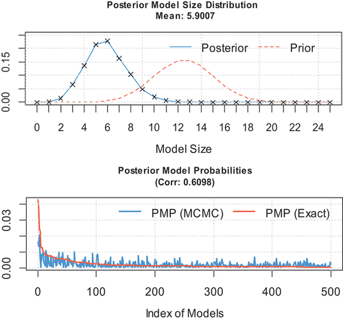
Table A5. Bayesian model averaging results with “flexible” g-prior

Code	PIP	Post Mean	Post SD
DCP	1.000	0.031	0.002
INFL	0.809	−0.029	0.018
GDS	0.424	0.044	0.064
LFP	0.328	−0.004	0.008
POPGR	0.312	0.000	0.000
CUCAC	0.247	0.731	1.754
INFRA	0.226	0.030	0.080
CROP	0.194	0.010	0.036
LR	0.181	−0.309	0.992
MARCA	0.179	0.002	0.017
GDPPER	0.168	−0.335	2.119
CAF	0.157	0.000	0.023
IMP	0.153	0.006	0.028
TAXPR	0.147	0.004	0.018
TOS	0.140	−0.004	0.036
DR	0.131	0.002	0.028
BM	0.125	−0.002	0.075
LIT	0.113	6.107	56.103
ATAX	0.110	0.001	0.006
DEBTSER	0.099	−0.003	0.048
Exp	0.099	−0.002	0.018
TST	0.099	−0.006	0.327
PERCA	0.099	0.003	0.023
DEBT	0.091	−0.001	0.006
NDEPO	0.083	0.008	0.334

Source: Author’s Construct, (2022)

Table A6. Bayesian model averaging results with “hyper” g-prior

Code	PIP	Post Mean	Post SD
DCP	1.00	0.032	0.001
INFL	0.86	−0.032	0.017
GDS	0.38	0.040	0.061
LFP	0.29	−0.004	0.007
POPGR	0.24	0.000	0.000
CROP	0.19	0.574	1.548
INFRA	0.16	0.021	0.067
PERCA	0.15	0.008	0.030
CUCAC	0.14	0.005	0.027
LR	0.12	−0.204	0.805
TST	0.11	0.002	0.337
TAXPR	0.11	0.002	0.014
GDPPER	0.11	−0.234	1.655
DR	0.10	0.003	0.024
LIT	0.10	5.887	51.741
IMP	0.09	0.004	0.022
BM	0.09	−0.003	0.062
MARCA	0.09	0.001	0.012
DEBTSER	0.09	−0.002	0.042
TOS	0.08	−0.003	0.026
NDEPO	0.08	0.008	0.316
ATAX	0.07	0.000	0.004
CAF	0.06	0.000	0.014
Exp	0.06	−0.001	0.012
DEBT	0.05	0.000	0.005

Source: Author’s Construct, (2022)

Table A7. Bayesian model averaging results with “EBL” g-prior

Codes	PIP	Post Mean	Post SD
DCP	1.000	0.032	0.001
INFL	0.782	−0.029	0.018
GDS	0.420	0.044	0.063
LFP	0.337	−0.005	0.008
POPGR	0.312	0.000	0.000
CROP	0.188	0.547	1.516
PERCA	0.157	0.008	0.031
BM	0.127	−0.005	0.074
DR	0.120	0.002	0.025
LR	0.117	−0.200	0.798
TST	0.114	−0.001	0.340
CUCAC	0.113	0.004	0.025
INFRA	0.108	0.013	0.053
LIT	0.099	5.230	49.988
TAXPR	0.097	0.002	0.014
IMP	0.090	0.003	0.021
GDPPER	0.086	−0.204	1.525
MARCA	0.083	0.001	0.011
NDEPO	0.081	0.006	0.315
Exp	0.079	−0.001	0.014
ATAX	0.078	0.000	0.005
DEBTSER	0.077	−0.002	0.039
DEBT	0.068	0.000	0.005
TOS	0.064	−0.002	0.024
CAF	0.050	0.000	0.012

Source: Author’s Construct, (2022)

References

- Adu, G., Marbuah, G., & Mensah, J. T. (2013). Financial development and economic growth in Ghana: Does the measure of financial development matter?. Review of Development Finance, 3(4), 192–21. https://doi.org/10.1016/j.rdf.2013.11.001
- Agrawal, P. (2000). Savings, investment, and growth in South Asia. India Gandhi Institute of Development Research.
- Ahmad, E., & Malik, A. (2009). Financial sector development and economic growth: An empirical analysis of developing countries. J Econ Cooperation Dev, 30, 17–40.
- Alfonso, H.-L. (2007). Infrastructure investment and Spanish economic growth, 1850–1935. Explorations in Economic History, 44(3), 452–468. https://doi.org/10.1016/j.eeh.2006.06.002
- Allen, F., Carletti, E., Cull, R., Qian, J., Senbet, L., & Valenzuela, P., 2012. Resolving the African financial development gap: Cross-country comparisons and a within country study of Kenya, NBER Working Paper Number 18013.
- Allen, D. S., & Ndikumana, L. (1998). Financial intermediation and economic growth in southern Africa, Working Papers 1998-004, Federal Reserve Bank of St. Louis.
- Amoah, L., Adjasi, C. K. D., Soumare, I., Osei, K. A., Abor, J. Y., Anarfo, E. B., Amo-Yartey, C., & Otchere, I. (2021). Finance, economic growth and development. In J. Y. Abor, C. K. D. Adjasi, & R. Lensink (Eds.), Contemporary issues in Development Finance (pp. 20–50). Routledge.
- Ang, J. B., & McKibbin, W. J. (2005). Financial liberalization, financial sector development and growth: Evidence from Malaysia”, Centre for Applied Macroeconomic analysis (CAMA) Working Paper 5, Australian National University.
- Caporale, G. M., Howells, P. G., & Soliman, A. M. (2004). Stock market development and economic growth: The causal linkages. Journal of Economic Development, 29(1), 33–50.
- Caporale, G., & Pittis, N. (1997). Causality and forecasting in incomplete system. Journal of Forecasting, 16(6), 425–437. https://doi.org/10.1002/(SICI)1099-131X(199711)16:6<425:AID-FOR657>3.0.CO;2-9
- Chowdhury, M. (2016). Financial development, remittances and economic growth: Evidence using a dynamic panel estimation. Margin: The Journal of Applied Economic Research, 10(1), 35–54. https://doi.org/10.1177/0973801015612666
- Čihák, M., Demirgüç-Kunt, A., Feyen, E., & Levine, R. (2012). Benchmarking financial systems around the World. World Bank, Policy Research Working Paper 6175
- Ehigiamusoe, U. K., & Lean, H. H. (2019). Do economic and financial integration stimulate economic growth: A critical survey. Economics—The Open Access Open-Assessment E-Journal, 13(4), 1–28.
- Esso, L. J. (2009). Cointegration and causality between financial development and economic growth: Evidence from ECOWAS countries. European Journal of Economics, finance and administrative sciences, 16.
- Fernandez, C., Ley, E., & Steel, M. (2001). Model uncertainty in cross-country growth regressions. Journal of Applied Econometrics, 16(5), 563–576.
- Gerschenkron, A. (1962). Economic backwardness in historical perspective. : Belknap Press of Harvard University Press.
- Ibrahim, M., & Alagidede, I. P. (2019). Asymmetric effects of financial development on economic growth in Ghana. The Journal of Sustainable Finance, 10(4), 371–387. https://doi.org/10.1080/20430795.2019.1706142
- Jiang, Y. (2011). Understanding openness and productivity growth in China: An empirical study of the Chinese provinces. China Economic Review, 22(3), 290–298. https://doi.org/10.1016/j.chieco.2011.03.001
- Kar, M., Nazlıoğlu, S., & Hüseyin, A. (2011). Financial development and economic growth nexus in the MENA countries: Bootstrap panel granger causality analysis. Economic Modelling, 28(1–2), 685–693. https://doi.org/10.1016/j.econmod.2010.05.015
- Khan, M. A., & Qayyum, A. (2006). ‘Trade liberalization, financial sector reforms, and growth’. Pakistan Development Review, 45(2), 711–731. https://doi.org/10.30541/v45i4IIpp.711-731
- Khan, M. A., Qayyum, A., Sheikh, S. A., & Siddique, O. (2005). Financial development and economic growth: The case of Pakistan [with comments]. Pakistan Development Review, 44(4), 819–837. https://doi.org/10.30541/v44i4IIpp.819-837
- Khan, S. M., & Senhadji, A. S. (2003). Financial development and economic growth: A Review and new evidence. Journal of African Economies, 12(AERC Supplement 2), ii89–ii110. https://doi.org/10.1093/jae/12.suppl_2.ii89
- Kiran, B., Yavus, N. C., & Guris, B. (2009). Financial development and economic growth: A panel data analysis of emerging countries. International Research Journal of Finance & Economics, 30, 1450–2887.
- Kohei, D., & Ken, T. (2013) Public infrastructure, production organization, and economic development. Journal of Macroeconomics, In Press, Corrected Proof, Available online http://ac.els-cdn.com/S0164070413001584/1-s2.0-S0164070413001584-main.pdf?_tid=18e5ddb0-4535-11e3-904a-00000aacb35f&acdnat=1383558190_b065ede9dad109577db5cfd0bc2285ad
- Lewis, W. A. (1954). Economic development with unlimited supplies, of labour. The Manchester School, 22(2), 139–191. https://doi.org/10.1111/j.1467-9957.1954.tb00021.x
- Liang, Q., & Jian-Zhou, T. (2006). Financial development and economic growth: Evidence from China. China Economic Review, 17(4), 395–411. https://doi.org/10.1016/j.chieco.2005.09.003
- Lloyd, P. J., & MacLaren, D. (2000). Openness and growth in East Asia after the Asian crisis. Journal of Asian Economics, 11(1), 89–105. https://doi.org/10.1016/S1049-0078(00)00042-7
- McKinnon, R. I. (1973). Money and capital in economic development. The Brookings Institution.
- Odhiambo, N. M. (2008). Financial depth, savings and economic growth in Kenya: A dynamic causal relationship. Economic Modelling, 25(4), 704–713. https://doi.org/10.1016/j.econmod.2007.10.009
- Patrick, H. T. (1966). Financial development and economic growth in underdeveloped countries. Economic Development and Cultural Change, 14(1), 174–189. https://doi.org/10.1086/450153
- Pradhan Rudra, P., & Bagchi Tapan, P. (2013). Effect of transportation infrastructure on economic growth in India: The VECM approach. Research in Transportation Economics, 38(1), 139–148. https://doi.org/10.1016/j.retrec.2012.05.008
- Quartey, P., & Prah, F. (2008). Financial development and economic growth in Ghana: Is there a causal link? African Finance Journal, 10(1), 28–54.
- Raftery, A. E., Madigan, D., & Hoeting, J. A. (1997). Bayesian model averaging for linear regression models. Journal of the American Statistical Association, 92(437), 179–191. https://doi.org/10.1080/01621459.1997.10473615
- Rask, J. K., & Rask, N. (2011). Economic development and food production–consumption balance: A growing global challenge. Food Policy, 36(2), 186–196. https://doi.org/10.1016/j.foodpol.2010.11.015
- Samargandi, N., Fidrmuc, J., & Ghosh, S. (2015). Is the relationship between financial development and economic growth monotonic? Evidence from a sample of middle‐income countries. World Development.
- Schumpeter, J. (1912). The theory of economic development. Harvard University Press.
- Shaw, E. S. (1973). Financial deepening in economic development. Oxford University Press.
- Uddin, G. S., Sjö, B., & Shahbaz, M. (2013). The causal nexus between financial development and economic growth in Kenya. Economic Modelling, 35, 701–707. https://doi.org/10.1016/j.econmod.2013.08.031
- World Bank. (1981). World development report. Oxford University Press,
- World Bank. (2012). World development report. Oxford University Press,
- Zhang, J., Wang, L., & Wang, S. (2012). Financial development and economic growth: Recent evidence from China. Journal of Comparative Economics, 40(3), 393–412. https://doi.org/10.1016/j.jce.2012.01.001