Forecasting Indian Goods and Services Tax revenue using TBATS, ETS, Neural Networks, and hybrid time series models

Abstract

This study focuses on the crucial task of forecasting tax revenue for India, specifically the Goods and Services Tax (GST), which plays a pivotal role in fiscal spending and taxation policymaking. Practically, the GST time series datasets exhibit linear and non-linear fluctuations due to the dynamic economic environment, changes in tax rates and tax base, and tax non-compliance, posing challenges for accurate forecasting. Traditional time-series forecasting methods like ARIMA, assuming linearity, often yield inaccurate results. To address this, we explore alternative forecasting models, including Trigonometric Seasonality Box-Cox Transformation ARIMA errors Trend Seasonal components (TBATS) and Neural Networks: Artificial Neural Networks (ANN), Neural Networks for Autoregression (NNAR), which capture both linear and non-linear relationships. First, we test single time series models like Exponential Smoothing (ETS), TBATS, ANN, and NNAR. Second, we also test hybrid models combining linear models, non-linear models, and neural network models. The findings reveal that the Hybrid Theta-TBATS model offers superior forecasting accuracy, challenging recent research favouring neural network models. The study highlights the effectiveness of advanced non-linear models, particularly TBATS and its hybridisations with linear models, in GST revenue forecasting. Our study also found that the single TBATS is the second-best model, which offers better forecasting accuracy. These insights have significant implications for policymakers and researchers in taxation and fiscal planning, emphasising the need to incorporate non-linear dynamics and advanced modelling techniques to enhance the accuracy of GST revenue forecasts.

Keywords:

• Non-linear models
• Neural Networks
• forecasting
• TBATS
• hybrid models
• Hybrid Theta-TBATS
• Machine Learning
• GST
• Goods and Services Tax

1. Introduction

A well-functioning tax system is a critical prerequisite for any country’s development beyond merely mobilising revenue (Diamond & Mirrlees, 1971). Tax revenue has been a vital source of income for both the state government and central government in India (Mukherjee, 2015). Despite various efforts to improve the Indian indirect tax structure, such as the introduction of the Central VAT (CENVAT),¹ reduction of the Central Sales Tax (CST) rate from 4% to 2%, and replacement of the single-point state sales tax with VAT, the origin-based Value Added Tax (VAT) system has numerous limitations (Mukherjee, 2019). These limitations and the complexity of the pre-GST indirect tax regime necessitated significant changes (Mukherjee, 2020a). The system before GST was burdened with multiple levies at the union and state levels, resulting in several non-compliances (Mukherjee, 2020b). Consequently, India transitioned to a destination-based Goods and Services Tax (GST) from 1 July 2017 onwards, which was viewed as a significant step toward transforming the country’s tax system into a comprehensive, efficient, transparent, and business-friendly system (Cnossen, 2013). Thus, implementing GST in India epitomised a crucial milestone in the country’s quest for a robust tax system.

Both in previous and current indirect tax systems, researchers and policymakers have been finding it difficult to forecast state-level and federal-level indirect tax revenue, tax efficiency, and/or tax capacity (Mukherjee, 2019). When digging out the existing literature, it is evident that most GST and indirect tax research have been conducted to predict tax capacity and efficiency (or inefficiency) using Stochastic Frontier Analysis (SFA) or tax buoyancy estimations. Besides, extant literature shows only a limited number of econometric models to predict Indian GST/VAT revenues—regardless of whether they are conducted using the pre-GST or post-GST datasets, and whether they are empirically examined at the state or national level. So far, no solid evidence exists that Indian aggregate GST revenue collection can be predicted/modelled solely by time series or panel data models. One reason could be that there are fewer post-GST time-series data points. Only a few researchers have attempted to estimate or predict GST/VAT-related variables. They include GST/VAT capacity (Mukherjee, 2019, 2020a), tax buoyancy (Paliwal et al., 2019), and tax efforts (Purohit, 2006). Interestingly, most existing academic contributions in the Indian context did not attempt to forecast the aggregate level of indirect tax revenue collections. Also, our extensive academic literature search yielded no empirical models for forecasting India’s monthly/yearly time-series indirect tax collections—neither on the pre-and post-GST datasets nor at the state-level datasets.

Bhattacharyya et al. (2022) note that there are two approaches to predict time series: (a) single model forecasting and (b) merging forecasting results of two or more models (hybridisation). Time series models use historical data points and extrapolate into the future (Bhattacharyya et al., 2022). Yet, we cannot expect the past to continue in the future. For example, the dynamic economic environment, changes in tax rates and tax base, and large tax non-compliance often cause non-linear fluctuations in the aggregate GST time series datasets, making GST/VAT revenue forecasting arduous (Dey, 2021; Mukherjee, 2020a). Extant literature shows that scholars have faced significant challenges in forecasting indirect tax revenue (GST/VAT) due to its non-linear and non-stationary nature (e.g., Dey, 2021). Methodologically speaking, the most widely used classical time series models, such as ARIMA and Theta methods, assume a linear relationship between past and future values (Khashei & Bijari, 2011; Navas Thorakkattle et al., 2022). This assumption is often violated in practice, leading to inaccurate forecasts (Ahmed et al., 2010). Time series data sets often contain linear and non-linear patterns, making it difficult for a single model like ARIMA to predict both linear and non-linear patterns of univariate datasets (Callen et al., 1996; Perone, 2021). Many recent studies used the linear Theta method, an alternative to the traditional linear ARIMA model, as yet another popular linear forecasting method for capturing “Trends” and “Seasonality” in time series data (Assimakopoulos & Nikolopoulos, 2000). It uses theta transformation to capture the long-term and short-term data features, identify complex patterns, handle non-stationarity, and detect and handle outliers in the time series dataset (Bhattacharyya et al., 2022).

Econometricians have recently begun using individual non-linear time series models, machine-learning-based time series models and hybrid (merging neural networks and traditional linear models) time series models as alternatives to linear models (Bhattacharyya et al., 2022; Perone, 2021). In this study, we considered traditional individual non-linear models such as Trigonometric Seasonality Box-Cox Transformation ARIMA errors Trend Seasonal components (TBATS) and ExponenTial Smoothing (ETS), which are now being widely used in stochastic time series forecasting (see Bhattacharyya et al., 2022; Perone, 2021). Likewise, hybridisation between linear, non-linear and neural network models is now widely attempted. The first non-linear model considered in our study, TBATS, handles multiple seasonality and complex patterns in data (De Livera et al., 2011). It uses Box-Cox transformation to help capture “Trends” and “Seasonality” (Bhattacharyya et al., 2021). It also models residuals as an ARMA process to de-correlate the time series data (Chakraborty et al., 2022). Subsequently, ETS is another non-linear time series model we tested in our forecasting exercise. It uses standard exponential smoothing techniques like Hold & Holt-Winters additive, multiplicative, or both methods (Fantazzini, 2020). ETS has a limitation of ineffective forecasting accuracy for short-term time series if the forecasting horizon is increased (Fantazzini, 2020).

Modern machine learning and hybrid models are empirically proven to be superior for time series forecasting (Kim et al., 2022). Artificial Neural Networks (ANNs) and Neural Network Auto-Regression (NNAR) are two of the widely applied machine learning models in time series forecasting (Bhattacharyya et al., 2022; Perone, 2021). Both models are non-linear models, which give better prediction accuracy. However, NNAR is typically superior to ANN, especially when the time series is non-linear (Zhang, 2003). The literature emphasises that neural network models can capture unobserved effects that linear time series like ARIMA models cannot. Deducting from such support, we assume the machine learning model is superior in predicting time series data. Alongside, hybridising forecasting models is not new, and their empirical applications resulted in superior forecasts to their counterparts (Perone, 2021). Most recently, a hybrid model (Theta-ARNN) combining linear and non-linear time series models had been proposed for COVID-19 and performed exceptionally well in predicting epidemics (Bhattacharyya et al., 2022). Perone (2021) also found that hybrid models performed better at capturing linear, non-linear, and seasonal pandemic patterns, outperforming all individual time series models. We also find that most time-series neural network studies use ANN and NNAR methods to forecast datasets (see Aranha & Bolar, 2023; Perone, 2021; Wagdi et al., 2023). This leads us to our research question: Can standalone neural network time series models and their hybridisation with linear time-series models outperform conventional single non-linear time-series models or their hybridisation with linear time series models?

Motivated by this, our study considers the monthly time series datasets of Indian Federal GST Revenue that displayed “non-stationary”, “non-linear”, and “non-Gaussian” patterns. The policymaking based on such a discrete model using such data will be unreliable and dicey. Hence, the first objective of this study is to propose a short-term non-linear time series forecasting model by comparing the forecasting performance of the individual non-linear models and neural network time series models (from among ETS, TBATS, ANN, and NNAR) that offer better monthly federal GST revenue forecasts. Second, we aim to compare the forecasting performance of hybrid models blending linear and non-linear models (from among Hybrid ARIMA-NNAR, Hybrid ARIMA-ANN, Hybrid Theta-ANN, Hybrid Theta-NNAR, and Hybrid Theta-TBATS) and propose one best hybrid model.

Our research contributes in several ways to the literature of the econometrics discipline. In this study, we propose a novel Hybrid Theta-TBATS model for short-term univariate GST revenue forecasting. We apply nine-time series models on a univariate dataset of monthly Indian GST revenue from July 2017 to November 2022. This article is the first to have tested the Indian GST time series data considering non-linear models, neural network models, and hybrid time series models. Our study included two non-linear models—ETS (multiplicative) and TBATS; and two neural network models—ANNs and NNAR. Among the four individual models, the TBATS model outperformed all other models. Hence, we propose non-linear TBATS as the best “single” model for accurately forecasting monthly GST revenue. Interestingly, we did not find neural network models (ANN and NNAR) superior in predicting time series GST data. In this study, we also hybridise linear time series like ARIMA and Theta between neural networks (ANN and NNAR) models and linear and non-linear time series models (Theta and TBATS) to identify the best hybrid forecasting model. The hybrid models considered in our model are ARIMA-NNAR, ARIMA-ANN, Theta-ANN, Theta-NNAR, and Theta-TBATS, formulated to capture both linear and non-linear dynamics of GST revenue collections. In our study, unexpectedly, the hybridisation of “Theta” and “TBATS” (not neural network models) exhibited the highest forecasting accuracy among all other “hybrid” models. Linear theta model captures the linear components of the datasets, while the non-linear model TBATS captures the non-linear components. Hence, we propose Hybrid Theta-TBATS as the best model for short-term monthly GST revenue forecasting among the nine models considered. Our research also found that TBATS “is” the best single model for prediction.

2. Literature Review

2.1. Goods and Services Tax in India

According to Rao (2000), the most significant challenge in reforming the Indian tax system is developing a coordinated indirect tax regime. GST is one of the most remarkable tax reforms in the Indian Tax system post 1991 (Mukherjee, 2020a; Rao et al., 2019). Vasanthagopal’s (2011) seminal study underscored the urgency of substituting India’s conventional origin-based value-added tax (VAT) regime with a destination-based goods and Services Tax (GST) system. His research shows how a destination-based GST can improve tax compliance, reduce tax cascading, and boost economic growth. It should simplify India’s consumption tax regime. GST became the primary source of indirect tax revenue collection after its implementation as a new indirect tax regime (Mukherjee, 2019, 2020a). Kumar et al. (2019) noted that GST is a dual VAT system with concurrent taxation powers for the centre and state governments, and it includes various taxes from both the centre and the state indirect tax bases.

According to Mukherjee (2020b), adopting a destination-based consumption tax system within the GST expects to promote investment and abridge the process of conducting business in India. GST regime absorbed more than a dozen state levies and completely restructured indirect taxes (except for customs duties) (Paliwal et al., 2019). The GST Council of India is in charge of determining tax rates, and it implements and collects GST using a cooperative fiscal federalism approach (Sharma, 2021). Nevertheless, India’s concurrent dual-GST system has been exacerbating political unwillingness, a lack of skilled labour, a lack of clarity in GST provisions, and a lack of policy for proper tax divisions (Kumar et al., 2019).

GST is a destination-based consumption tax levied on goods and services at various stages of production and distribution, with taxes on inputs credited versus taxes on output (Mukherjee, 2020a, 2020b). GST now follows cooperative federalism. It is implemented to ensure India’s balanced economic development by simplifying the complex indirect tax system, allowing commodities to move freely across state and national borders, reducing tax evasion and expanding the taxpayer base, improving compliance with taxation rules, increasing government revenues, and attracting investors by making it easier to do business in India (Singhal et al., 2022). Unlike other GST structures in the world, India has a dual GST structure,² in which the central and state governments both levy taxes (Garg et al., 2017). Hence, GST consists of Central GST (CGST), State GST (SGST)/Union Territory GST (UTGST), and Integrated GST (IGST).³ GST has changed the federal tax system and harmonised a mosaic of central and state levies, replacing the chaotic indirect structure that significantly increased product prices. Over 160 countries have implemented the GST indirect taxation system (Revathi & Aithal, 2019). However, developmental economists warn that an exogenous increase in taxes on percentage GDP would reduce the real GDP by almost three per cent (e.g., Romer & Romer, 2010). Therefore, the implementation should be cautious.

2.2. VAT/GST research in India so far

Any consumption tax is imposed based on the GSDP, investment, export from the state, import to the state, and government public expenditure (Jha et al., 19991999; Mukherjee, 2020a). That is, the potential for GST revenue mobilisation is based on the GST capacity and potential one state offers. That could be improved per capita GDP, the states’ Special Category status, and technical efficiency in mobilising GST revenues (Mukherjee, 2019, 2020a). Mawejje and Sebudde (2019) found that high-income levels, a large share of non-agricultural outputs, an increased share of trade in GDP, higher investment in human development, developed financial sectors, a stable domestic environment (low and stable inflation), lower corruption, and a higher urbanised population are all factors that contribute to the revenue of a state. Using the regression approach, Oommen (1987) measured the tax efforts of 16 major states from 1970 to 1982. The researcher compared State Tax and State Domestic Gross Product (SDGP) to assess tax elasticity and tax buoyancy as tax base indicators. Furthermore, regression models were employed to calculate the residual (the disparity between the actual tax revenue vis-à-vis income ratio and the estimated tax revenue vis-à-vis income ratio) to measure tax effort. The findings indicated a need for further scrutiny and ongoing examination of the comparative tax efforts among Indian states.

2.3. Empirical modelling in GST/VAT research

The tax revenue potentials, tax efforts, and tax collection efficiency are widely measured using the Stochastic Production Frontier Analysis (SFA) (Aigner et al., 1977). Meeusen and van Den Broeck (1977) incorporated the SFA into Cobb-Douglas production models that included a composed error. Jha et al. (1999) measured the pure tax efficiency of 15 major Indian states between 1980–81 and 1992–93. A time-variant SFA was adopted in that study to test and estimate tax efficiency. They found that the State Domestic Products (SDP), the proportion of agriculture, income to total SDP, and time series trend are the major factors determining a state’s Own Tax Revenue (OTR). It also established a positive correlation between SDP and OTR and a negative correlation between the proportion of agricultural output in SDP and OTR. Purohit (2006) ranked the Indian states based on tax efforts using the income approach. State governments’ tax efforts and taxable capacity are also compared across all Indian states. Several tax base determinants were chosen to estimate the average tax rate, taxable effort, and state taxable capacity. During the study period of 2000–2003, Gujarat ranked first in terms of taxable capacity and tax efforts, followed by West Bengal and Andhra Pradesh. In their study spanning the years 2000–2011, Karnik and Raju (2015) employed time-invariant SFA to estimate tax capacity of 17 prominent Indian states without including efficiency factors in their model. Their discoveries reveal that the proportion of manufacturing in Gross State Domestic Product (GSDP) and yearly per capita consumption expenditure are the principal determinants of sales tax, expressed as a percentage of GDP.

Utilising SFA, Garg et al. (2017) conducted a study on tax capacity and tax efforts of 14 major Indian states between 1992–1993 and 2010–11. Their findings indicate that per capita real GSDP, the proportion of agricultural output in GSDP, literacy rate, labour force, road density, and urban Gini coefficient (a metric of consumption inequality) have a significant impact on OTR collection by states, except for the squared per capita real GSDP and the share of agriculture in GSDP. All other independent variables are directly and significantly associated with their tax revenue mobilisation. Mukherjee (2019) modelled the state’s VAT tax capacity as a function of its economic activity scale (GSDP) and structural composition from 2000–01 through 2015–16. The panel SFA result revealed that VAT capacity is lower in states with a higher share of manufacturing and mining activities or industry in GSDP compared to agriculture and higher in states with a higher share of service in GSDP vis-a-vis agriculture in GSDP. A VAT revenue is estimated as a product of a state’s applicable tax rate and total private consumption expenditure (tC) minus the VAT rate on exports to other states (Xt₁). The final consumption expenditure (tC) is calculated as GSDP—Investment (I)—Export to other states (X)—Government consumption expenditure (G) + imports from other states (M). Because a state’s export (X) is difficult to quantify, it is calculated as the function of mining, quarrying, manufacturing, and services with agriculture in that state.

Mukherjee (2020a) again examined the tax capacity and tax efficiency of Indian states by applying time-variant truncated panel SFA. The author took logGST as the dependent variable. He slightly modified his Mukherjee (2019) measurement to estimate the GST revenue by replacing GSDP with GSVA. The independent variables in the model were manufacturing/agriculture, service/agriculture, industry/agriculture, and mining/agriculture to show the export potential of Indian states. Besides, to account for the first three quarters of the initial GST Year (FY 2017–18), the author brought in a dummy = 0.75, and the rest of the year takes “1”. The SFA model’s tax collection inefficiency term (Ui) was separately predicted using the log of per capita GSVA and special category state status (dummy coded). The investigation discovered that minor states have lower tax efficiency (or higher tax inefficiency), and Delhi and Goa have had the highest GST Gap. It found that the average GST revenue of all major states grew by 0.52% of GSVA for the sample year.

Kawadia and Suryawanshi (2023) applied SFA to identify the tax capacity and tax efforts of Indian states from 2001–2002 through 2016–2017. It found that GST “tax capacity” is significantly influenced by per capita income, infrastructure, agricultural activity, labour force, and bank credit. In contrast, tax effort is influenced by social sector spending and federal transfers (in-grant) to states. Besides, states’ taxing authority has been reduced due to the GST. Consequently, for revenue mobilisation, the states heavily rely on their limited legislative taxes, which are insufficient to meet their needs. They also argue that all states have achieved at least 90 per cent of their tax potential, leaving little room for the subnational governments to raise more revenue through taxation.

2.4. Univariate time series forecasting

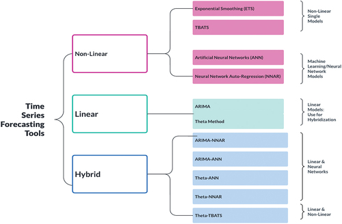
In this section, we review well-cited literature relating to the most commonly used models in our research, such as linear models: ARIMA and Theta method (used for hybridisation to capture linear components); non-linear models: ETS, TBATS; Neural Networks: ANNs and NNAR; and Hybrid models. Remember that we have not reviewed the literature on all available time series models. As shown in Figure 1, we restricted our reviews of time series models based on the accuracy of our forecast result despite having access to abundant literature.

Figure 1. Time series forecasting tools used in the study.

2.4.1. ARIMA and Theta method: Linear models

ARIMA is one of the popular linear models in time series forecasting applied during the past five decades (Zhang, 2003). The model assumes that the data will be linear and the error distribution will be homoscedastic (Bhattacharyya et al., 2022). As given by Perone (2021), the estimated equation for ARIMA is

${\mathrm{\Delta }}^d{y}_t={\varphi }_1{\mathrm{\Delta }}^d{y}_{t-1}+\dots {\varphi }_p{\mathrm{\Delta }}^d{y}_{t-p}+{\gamma }_1{\epsilon }_{t-1}+\dots {\gamma }_q{\epsilon }_{t-q}+{\epsilon }_{t,}$

where “${\mathrm{\Delta }}^d$”= second difference operator, “$y_t$” = predicted values, “$p$” = lag order of the AR process, “$\varphi$” = coefficient of each parameter “p”, “q” = order of the MA. “$\gamma$” = coefficient of each parameter q, and ${\epsilon }_{t,}$= residuals of the errors at the time “t”. We included ARIMA as a linear model as this model is widely used in econometrics and finance literature.

Theta method is another linear classical time series forecasting model that captures “Trends” and “Seasonality” in time series data (Assimakopoulos & Nikolopoulos, 2000; Hyndman & Billah, 2003). It applies theta transformation to capture long-term and short-term data features, complex patterns, non-stationarity, and outliers in time series datasets (Bhattacharyya et al., 2022;). The theta method decomposes the original data into two or more theta lines and extrapolates them (Hyndman & Billah, 2003). Spiliotis et al. (2020) suggested that the theta method is best for automatic time series forecasting. This theta is now used for economic forecasting, financial forecasting, sales forecasting, etc. (Hyndman & Athanasopoulos, 2018). Remember, we included the literature on the ARIMA and Theta method to show that these two methods capture the linear component of the datasets. Moreover, we performed hybridisation of ARIMA-ANN, ARIMA-NNAR, Theta-TBATS, Theta-ANN, and Theta-NNAR. Hence, it is essential to give a brief background of these two time series models.

2.4.2. ETS and TBATS: Non-linear models

Error-trend-seasonal or ExponenTial Smoothing (ETS) methods have been applied in econometrics literature. ETS model devises standard exponential smoothing models following additive and multiplicative methods. ETS decomposes a time series “Y” into three components: a trend (T): long-term components, a seasonal pattern (S), and an error term €. It uses standard exponential smoothing techniques like Hold & Holt-Winters additive (Y=T+S+E), multiplicative (Y=T·S·E), or both (Y=T·S+E) methods. Here, we consider ETS as multiplicative smoothing. The equation for ETS for additive error is as follows:

Forecast Equation: ${\hat{y}}_{t+1\mid t}=l_t.$

Smoothing Equation: $l_t=l_{t-1}+\alpha \left(y_t-l_{t-1}\right)$,

where “$l_t$” = new estimated level, “${\hat{y}}_{t+1\mid t}$” =each one step-ahead prediction for time “t₊₁”, which results from the weighted average of all the observed data, 0 $\le \alpha \le 1$ is the smoothing parameter, which controls the rate of decrease of the weights, and “$y_t-l_{t-1}^{\prime }$” is the error at the time “t”. ETS provides good forecast accuracy for the short term, but the quality decreases if the forecasting horizon is increased (Fantazzini, 2020). Dey (2021) applied the ETS method to predict the monthly GST revenue of Odisha state (India) with a limited number of data points.

Trigonometric Seasonality Box-Cox Transformation ARIMA errors Trend Seasonal components (TBATS) is another advanced non-linear time series model capable of handling seasonality and complex patterns present in the data (De Livera et al., 2011). In this method, the Box-Cox transformation is applied to address the non-linearity and non-normality issues in the data and help to capture the underlying trend and seasonality in the data (Bhattacharyya et al., 2021, 2022). It models residuals as an ARMA process to de-correlate the time series data and forecast better (Chakraborty et al., 2022). TBATS combines various techniques to handle different aspects of time series data, such as non-linearity, non-normality, autocorrelation, and complex seasonality patterns. TBATS has been widely used when modelling for short-term forecasting (see COVID-19 prediction: Bhattacharyya et al., 2022; Perone, 2021). The statistical equations for TBATS, Theta method, and hybrid models are in Section 3.3.

2.4.3. ANN and NNAR: Neural network models

Neural network models have widely been used in diverse fields of study, including finance and economics (Ahmed et al., 2010; Chhajer et al., 2022; Thayyib et al., 2023). Such models are effective at forecasting non-linear data with complex patterns. Neural network models have significantly progressed in handling non-linear function estimation, pattern identification, optimisation, and simulation problems (Maniati et al., 2022). Sabri et al. (2022) argue that using complex algorithms, ANNs deliver superior solutions than standard statistical techniques. Given their benefits, neural network models have garnered interest in time series forecasting of various datasets (Khashei & Bijari, 2011). Such time series neural networks are effective at forecasting a variety of time series datasets, including stock prices (Blöthner & Larch, 2022; Cao & Wang, 2019; Du Plooy et al., 2021; Mostafa, 2010; Vijh et al., 2020), economic data (Aminian et al., 2006; Milačić et al., 2017), corporate bankruptcy data (Aranha & Bolar, 2023; Kim et al., 2022), currency exchange rates (Wagdi et al., 2023), weather data (Abhishek et al., 2012), water quality data (Faruk, 2010), and solar radiation data (Ghimire et al., 2019; Premalatha & Valan Arasu, 2016; Xue, 2017; Yadav & Chandel, 2014).

In the economics literature, Wagdi et al. (2023) integrated ANN and technical indicators for predicting the exchange rates of 24 emerging economies between January 2012 and November 2022. It found a significant improvement in the values predicted for exchange rates by ANN versus those predicted by technical indicators alone. It also found a significant difference between the values ANN predicted for exchange rates for emerging economies and the actual values based on currency. Aranha and Bolar (2023) applied ANN to check the forecasting performance of extant credit risk models. They found that Machine Learning Techniques are better than Logistic Regression in predicting the bankruptcy of firms and that the same predictive power of ascertaining bankruptcy improves when a proxy for uncertainty is added to the model. Du Plooy et al. (2021) discovered that ANNs could model complex non-linear relationships and are not bound by the restrictive assumptions of traditional time-series models in option pricing. Time series forecasting using ANNs suggests that ANNs can be a promising alternative to the traditional linear method. Lam and Oshodi (2016) found that the Neural Network Auto-Regressive (NNAR) model outperformed the conventional ARIMA when attempting to predict construction output.

Milačić et al. (2017) and Cadenas and Rivera (2010) have proven the success of utilising non-linear time series techniques such as ANNs and Auto-Regressive Neural Networks (ARNNs) in infectious disease modelling. Yadav and Chandel (2014) compared traditional and neural network methodologies to predict solar radiation. The study demonstrated that when using assessment measures like Root Mean Squared Error (RMSE) and Mean Absolute Percentage Error (MAPE), Deep neural network (DNN) models outperform all other methods in terms of producing accurate results. In another study, Ghimire et al. (2019) provided several models and techniques such as ANN, Genetic Programming (GP), Support Vector Regression (SVR), Deterministic Models (DM), Temperature Models (TM), and Gaussian Process Machine Learning (GPML) for medium range weather forecast fields in solar rich cities of Queensland, Australia. Xue (2017) introduced a Back Propagation Neural Network (BPNN) model with two optimisation algorithms named Genetic Algorithm (GA) and Particle swarm optimisation (PSO) for the prediction of daily diffuse solar radiation. Likewise, Premalatha and Valan Arasu (2016) also suggested an ANN-based forecasting model for solar radiation prediction that uses a back-propagation technique. These works employ MAE, RMSE, and Maximum Linear Correlation Coefficient (R) as assessment criteria for identifying the superior model. The results showed that the proposed BPNN optimised by the PSO model has the potential to predict the daily diffuse solar radiation accurately. Silva et al. (2019) attempted to predict the tourism demand using denoised Neural Networks. The study used the Automated Neural Network Autoregressive (NNAR) algorithm from the forecast package in R, which generates sub-optimal forecasts when faced with seasonal tourism demand data. They proposed denoising to improve the accuracy of NNAR forecasts via an application for forecasting monthly tourism demand for 10 European countries.

These articles show increasing interest in representing complex, non-linear cognitive functions using neural network models. However, compared to other statistical techniques, a few published studies still clearly explain a methodology for obtaining trustworthy taxation data modelling using neural networks because of the relatively new introduction of these models. Therefore, this study attempts to bridge this gap in the literature.

2.4.4. Hybrid time series models

Hybrid time series models capture linear and non-linear patterns in time series datasets (Ghasemiyeh et al., 2017; Khashei & Bijari, 2011; Wang et al., 2018). For example, Khashei and Bijari (2011) formed a hybrid model combining ARIMA and ANN to improve the time-series forecasting performance. Similarly, Li and Dai (2020) hybridised the Convolution Neural Network (CNN) and Long Short-Term Memory (LSTM) models to forecast the bitcoin price. They found that this hybrid model can effectively improve the accuracy of value and direction predictions compared with the single-structure neural network. The hybridisation of both ARIMA and neural networks has also been widely applied to time-series datasets (see, e.g., Faruk, 2010; Ghasemiyeh et al., 2017). Similarly, Zhang (2003) hybridised ARIMA and neural network models to use ARIMA and ANN to capture the datasets’ linear and non-linear dynamics. They found that hybridisation improves forecasting performance. Bhattacharyya et al. (2022) found that a hybrid formulated using the Theta Method and Auto-Regressive Neural Network (TARNN) best predicted the daily COVID-19 cases in five countries. In addition, the authors performed hybridisation between ARIMA-ARNN and ARIMA-Wavelet ARIMA (WARIMA). Perone (2021) found that NNAR-TBATS and ARIMA-NNAR are the two best hybrid forecasting models for short-term COVID-19 forecasting in Italy. However, Callen et al. (1996) found that neural network models were not outperforming linear time series models when forecasting quarterly earnings data. It indicates that it is not always necessary for hybrid models to be superior. In our study, we hybridise the models of machine-learning-based models as well as the linear and non-linear models.

In summary, the extant empirical literature in the Indian context has only a limited number of models examining GST revenue predictions. Most studies have employed SFA to determine inefficiencies in GST capacity and tax efforts at the state level, using panel data both for pre- and post-implementation. It could be because of fewer data points. Also, univariate linear and non-linear time-series modelling of Indian GST revenue collection is notably absent from the literature, except for Dey (2019), who applied the ETS method, a non-linear time series technique to predict revenue with limited data points. Nonetheless, no credible scholarly work has endeavoured to forecast GST revenue using linear and non-linear models, particularly by applying the recent neural network models and their hybridisations.

3. Methodology

Time series analysis begins with the trend, seasonality, outlier, and residual analysis (Zhang, 2003). Determining the accuracy of time series results from a single linear model or a single non-linear model is difficult. Hence, the hybridisation of linear and non-linear time series models is often tested and tested. The hybrid methodology is based on the additive relationship between linear and non-linear components of time series (Taskaya-Temizel & Casey, 2005).

3.1. Data source and constraints

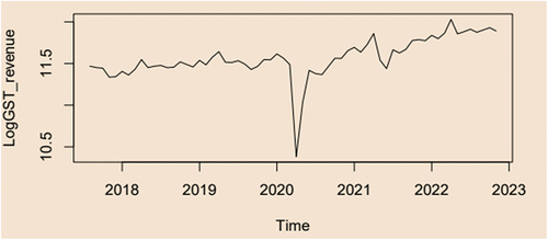
We collected monthly unaudited Gross GST revenue [combining State GST, Central GST, Integrated GST (includes GST on Goods import), Compensation Cess (includes GST on Goods import)] revenue from the Indiastats Database, which was cross-verified at the GST Council Website. As shown in Figure 2, we considered monthly collection from August 2017 to November 2022 as we attempted to propose the best forecasting models for monthly GST revenue. As this is aggregate federal-level data, we believe there is no scope for data constraints. But we could not test the result at state-level datasets to validate the result due to data discrepancies in the state-level datasets. States receive Inter-State GST (IGST) settlement from the Union Government, which is applied against tax liability in the destination state. Also, we could not get regular IGST settlement data for each month that we considered.

Figure 2. Time series plot of log GST data: this time series plot displays the log of the GST in constant prices, also known as the log GST data. Y-axis = the logGST, X-axis= Time.

There have been a variety of problems with state GST datasets. First, states collect revenue from taxes through State GST (SGST), with an anticipated annual growth rate of 14% (Mukherjee, 2020a). As per the Finance Commission’s tax devolution formula, states receive a portion of the net collection of Central GST (CGST) after accounting for refunds and collection costs. However, there are discrepancies between the SGST collection reported in State Finance Accounts (SFA) and the GSTN database. Moreover, tax revenue figures for various states subsumed in GST are unavailable.

3.2. Data and packages

The data sets were divided into two categories: “Training data” and “Testing data”, with the latter representing monthly datasets, observed post-GST implementation. Data sets exhibited non-linear and non-Gaussian behaviour, with a cyclical pattern and mean cycle of about one year. In our study, similar to Gholami et al. (2019), we split the training set, which comprised 70% of the dataset, which was used to build the models, and the testing dataset, which comprised the last 19 months (30%) of data to assess the forecasting performance of models. Single non-linear models like ETS and TBATS, neural networks like ANN and NNAR, and hybrid models were tested for forecasting performance accuracy.

Non-linear modelling with the NNAR approach is done with the “caret” package using the “nnetar” function and ANN with the “nnfor” package using the “mlp” function in R statistical software. Another single model, such as ETS and TBATS, is done in R software using the package “forecast”, and the function is “ets” and “tbats”, respectively. Hybridisation Codes are given in Appendix A. We explain below the two best models out of nine that were significant in our forecasting attempt.

3.3. Econometric models

Our study picks out two prominent models with better forecasting accuracy. Therefore, we only explain the linear model: (a) Theta (however, not tested individually as our data is non-linear); non-linear model (b) TBATS; (c) Hybrid Theta-TBATS. For Hybrid Theta-TBATS, we explain how we formulated the Theta-TBATS hybridisation model.

3.3.1. Theta model

The Theta model, created by Assimakopoulos and Nikolopoulos (2000), is a univariate forecasting technique that utilises the Theta transformation. It involves dividing the original data into two or more lines (called Theta lines) and extrapolating them by forecasting models (Bhattacharyya et al., 2022). The predictions from each line are then combined to produce the final forecasts (Chakraborty et al., 2020). Theta model has since been used in various forecasting applications and has gained popularity for its ability to capture both “trend” and “seasonality” in time series data. The mathematical expression for the Theta model is provided below:

$\begin{array}{c}{\mathrm{\nabla }}^2{Z}_t\left(\theta \right)=\theta {\mathrm{\nabla }}^2{Y}_t=\theta \left(Y_t-2Y_{t-1}+Y_{t+2}\right),t=3\dots n\\ Z_t\left(\theta \right)=\theta Y_t+\left(1-\theta \right)Z_t\left(0\right)=\theta Y_t+\left(1-\theta \right)\left(A_n+B_{n}t\right),t=1\dots ,n,\end{array}$

where “${\mathrm{\nabla }}^2{Y}_t$” are the second differences between the original series “Y” and “$\left\{A_n,B_n\right\}$” are the intercept and the slope Expression for “$\left\{A_n,B_n\right\}$” is

$\begin{array}{c}{A}_n=\frac{1}{n}\sum _{t=1}^n{Y}_t-\frac{n+1}{2}{B}_n,\\ B_n=\frac{6}{n^2-1}\left(\frac{2}{n}\sum _{t=1}^{n}t{Y}_t-\frac{1+n}{n}\sum _{t=1}^n{Y}_t\right),\end{array}$

Theta transformation is a powerful tool in time series forecasting, as it can effectively capture the long-term and short-term characteristics of the data, identify complex patterns, handle non-stationarity, and detect and handle outliers. Its ability to combine multiple forecasting models also makes it a versatile and robust method for time series analysis.

3.3.2. TBATS model

The TBATS model is a state-of-the-art time series forecasting model that can handle multiple seasonality and complex trend patterns in the data (De Livera et al., 2011). In this advanced non-linear time series forecasting method, the Box-Cox transformation handles non-linearity and non-normality in the data. By transforming the data using the Box-Cox transformation, the model can more effectively capture the underlying trend and seasonality patterns (Bhattacharyya et al., 2021). The ARMA model captures the remaining autocorrelation in the residuals after removing the trend and seasonality components. By modelling the residuals as an ARMA process, the model can de-correlate the time series data and make better predictions for future periods (Chakraborty et al., 2022). TBATS model combines various techniques to handle different aspects of time series data, such as non-linearity, non-normality, autocorrelation, and complex seasonality patterns. According to Perone (2021), the basic TBATS equation forms the following forms:

$y_t^{\left(\omega \right)}=1_{t-1}+\varphi b_{t-1}+\sum _{i=1}^T{s}_{t-m_i}^{\left(i\right)}+d_t,$

where $y_t^{\left(\omega \right)}$ specifies the Box-Cox transformation parameter (ω) applied to the observation y_t at time t, i_t is the local level, $\varphi$ = damped trend, b = long-run trend, T = seasonal pattern, $s_t^{\left(i\right)}$ = ith seasonal component, $m_i$ = seasonal periods, and $d_t$ = ARMA (p,q) process for residuals.

The trigonometric expression of seasonality terms is a more flexible way to model complex seasonality patterns than simple seasonal dummies. The trigonometric expression can model both low-frequency and high-frequency seasonality patterns and requires fewer parameters than using seasonal dummies. This makes the model more parsimonious and reduces the risk of overfitting the data.

3.3.3. Hybrid model formulation

The hybrid approach seeks to enhance the accuracy and reliability of forecasting methods by combining the strengths of multiple models and mitigating the limitations of individual models (Callen et al., 1996; Perone, 2021). This approach holds significant practical value across diverse domains, including finance, economics, and weather forecasting, where precise time series forecasting is crucial (Taskaya-Temizel & Casey, 2005). The hybrid model (Z_t) can be represented as follows:

$Z_t=Y_t+N_t,$

The hybrid model decomposes the time series into two components: a linear component, denoted as “Y_t”, and a non-linear component, denoted as “N_t”. These two components are estimated from the data using appropriate techniques. The forecast value of the linear model at the time “t” is denoted as “${\hat{Y}}_t$,” and the residual at a time “t” from the linear model is represented as “ε_t”. These values are used to model the linear component of the hybrid model, “Y_t”. The error term of “ε_t” is defined as

${\epsilon }_t=Z_t-{\hat{Y}}_t,$

For the Theta-TBATS model, “${\hat{Y}}_t$” be the forecast value of the Theta model at the time “t” and “${\epsilon }_t$” represents the residual at the time “t” obtained from the Theta model.

The residuals are modelled as follows:

${\epsilon }_t=f\left({\epsilon }_{t-1},{\epsilon }_{t-2},\dots ,{\epsilon }_{t-n}\right)+{\zeta }_t,$

where “f” is a non-linear function modelled by the non-linear TBATS and “ς_t” is the random error. Therefore, the combined forecast is

${\hat{Z}}_t={\hat{Y}}_t+{\hat{N}}_t,$

where “${\hat{N}}_t$” = forecast value of the Theta model.

The rationale for using residuals to assess the adequacy of the proposed hybrid model is that the residuals still contain autocorrelation, which the linear approach cannot model. The non-linear model, which can capture the non-linear autocorrelation relationship, performs this task. In our study, the Hybrid Theta-TBATS model operates in two distinct phases to achieve its goal. Initially, the model applies the Theta model to examine and analyse the linear component of the overall model. Next, in the second phase, a TBATS model is employed to capture and model the residuals that remain after applying the Theta model. Combining these two approaches, the hybrid model effectively addresses and minimises the inherent uncertainties associated with inferential statistics and time series forecasting.

3.4. Evaluation metrics

Our study uses three metrics to evaluate the performance of various forecasting models, including the proposed model. These metrics are RMSE, MAE, and MAPE. Their definitions are as follows:

Root Mean Square Error (RMSE): It measures the average difference between the predicted values and the actual values in the dataset, considering the squared differences between each predicted and the actual value (Vijh et al., 2020). The RMSE is calculated as follows:

$\mathrm{R}\mathrm{M}\mathrm{S}\mathrm{E}=\sqrt{\frac{1}{n}\sum _{i=1}^n{\left(y_i-{\hat{y}}_i\right)}^2},$

Mean Absolute Error (MAE): MAE calculates the average absolute difference between the dataset’s actual and predicted values (Premalatha & Valan Arasu, 2016). MAE measures the average magnitude of errors the model makes without considering their direction (Milunovich, 2020). A lower MAE indicates better model performance. The formula for MAE is

$\mathrm{M}\mathrm{A}\mathrm{E}=\frac{1}{n}\sum _{i=1}^n\left|y_i-{\hat{y}}_i\right|,$

Mean Absolute Percentage Error (MAPE): It measures the average percentage difference between the predicted and actual values in the dataset (Deb et al., 2017; Premalatha & Valan Arasu, 2016). The MAPE formula is

$\mathrm{M}\mathrm{A}\mathrm{P}\mathrm{E}=\frac{1}{n}\sum _{i=1}^n\left|\frac{y_i-{\hat{y}}_i}{y_i}\right|\times 100\mathrm{\%},$

MAPE measures the size of the errors relative to the actual values, which can be useful in cases where the scale of the data is important. A lower MAPE indicates better model performance.

Here, “$y_i$” = actual value, “${\hat{y}}_i$” = predicted value, and “n” = number of data points. The performance of the forecasting model improves as these values decrease.

3.5. Non-linearity tests

Determining whether time series data is linear or non-linear is an important step in analysing the data because the type of model and methods used for analysis will depend on the nature of the data. To check whether a time series data is linear or non-linear, use the “nonlinearity test” function within the “non-linear series” package in R to test for nonlinearity in time series data. The nonlinearity test function performs a battery of tests to check for nonlinearity in the time series data. The output of the function will indicate whether the null hypothesis of linearity can be rejected, with a p-value indicating the significance level.

Because the p-value is less than the significance level (p-value = 0.05) for all five tests, it is typically interpreted as evidence against the null hypothesis. In other words, there is substantial evidence that our monthly log GST data has a non-linear structure. As per Table 1, all the tests for non-linearity turned out to be significant; hence, the researcher confirms that the GST dataset has a non-linear data pattern.

Table 1. Test for non-linearity and p-value

Non-linearity tests	p-Value
Teraesvirta’s neural network test	0.027
White neural network test	0.012
Keenan’s one-degree test for nonlinearity	0.009
McLeod-Li test	1.20*10^−8
Tsay’s test for nonlinearity	0.009
Likelihood ratio test for threshold nonlinearity	0.018

4. Forecasting results

Our study aims to propose one single best model and one best hybrid model out of nine models such as TBATS, ETS, ANN, NNAR, ARIMA-ANN, ARIMA-NNAR, Theta-ANN, Theta-NNAR, and Theta-TBATS. According to Table 2 and Figure 3, the Hybrid Theta-TBATS model has the lowest RMSE, MAE, and MAPE values compared to all other tested models. The result implies that the Hybrid Theta-TBATS model provides the most accurate forecasts among all the nine models. The hybridisation of the Theta model and TBATS model would help predict the GST revenue better than linear vs neural network models such as ARIMA-ANN, ARIMA-NNAR, Theta-ANN, and Theta-NNAR. Similarly, the single TBATS (non-linear but not neural network) model was the second-best time series model to predict short-term monthly GST revenue. In this sense, TBATS, a non-linear time series prediction model, is the single best among the non-linear models and single neural network models.

Figure 3. RMSE plot for all nine models.

Note. X-axis: Forecast Horizon; Y-axis: RMSE Value.

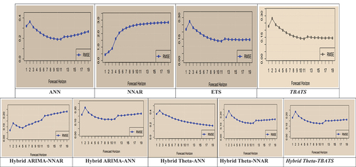
Table 2. Model validation of log GST data of India

Model	RMSE	MAE	MAPE
ANN	0.271	0.237	2.010
NNAR	2.758	2.638	22.314
ETS	0.146	0.124	1.053
TBATS (Proposed Single)	0.145	0.120	1.017
Hybrid ARIMA-NNAR	0.231	0.207	1.754
Hybrid ARIMA-ANN	0.296	0.275	2.32
Hybrid Theta-ANN	0.147	0.125	1.062
Hybrid Theta-NNAR	0.160	0.143	1.20
Hybrid Theta-TBATS (Proposed Hybrid)	0.141	0.114	0.971

RMSE = root mean square Error; MAE = mean absolute Error; MAPE = mean absolute percentage error.

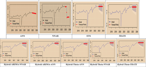
Figure 4 depicts the forecasted values of log GST data for the next 12 months using all nine models, including non-linear time-series models, neural networks, and hybridisation of linear and non-linear/neural networks. To summarise, we examined the monthly GST time series datasets that exhibited non-linear and non-Gaussian behaviour with a cyclical pattern. We compared the forecasting accuracy of linear and non-linear time series single models, including ETS, TBATS, ANN, and NNAR, to forecast future values. The study found that the neural network hybrid models ARIMA-NNAR, ARIMA-ANN, Theta-NNAR, and Theta-ANN models did not perform better. Instead, Hybrid Theta-TBATS performed best among all nine models. Table 2 reveals that a combination of linear Theta and non-linear TBATs model (RMSE = 0.141; MAE = 0.114; MAPE = 0.971) is the best to predict monthly GST tax revenue collection, followed by the TBATS (RMSE = 0.145; MAE = 0.120; MAPE = 1.017). Remember, our GST datasets exhibited a “non-stationary”, “non-linear”, and “non-Gaussian” nature. Hence, we disregarded the individual results of individual ARIMA and Theta Method, which assume the linearity of time series.

Figure 4. Actual vs 12-month forecasts data points for all nine models.

Note. X-Axis: Year and Y-Axis: LogGST Revenue.

Hybridisation combines the benefits of two distinct models to improve forecasting performance. In fact, the hybridisation of models is not new in univariate time series forecasting. However, the novelty in our study is that our forecasting result decries the superiority of single neural network models and their hybridisations. Instead, the hybridisation of one linear model viz Theta Method and one non-linear mode viz TBATS was the best among all five hybrid models. Hence, the hybrid Theta-TBATS is a significant contribution to econometric modelling literature. Similarly, the non-linear TBATS model was the best single model for revenue forecasting. Hence, the two models offer significant implications for indirect revenue forecasting and tax policy decision-making.

5. Conclusions

Our fundamental research question in this study was whether neural network time series models and their hybridisation with linear time-series models outperform conventional single non-linear time-series models or their hybridisation with linear time series models. The finding does not show any evidence for superior forecasting performance by ANN and NNAR or their hybridisation with linear models. Instead, in this study, we propose a novel Hybrid Theta-TBATS model for short-term univariate GST revenue forecasting. This study used nine different neural network models to attempt a short-term 12-month univariate forecasting of India’s monthly federal GST revenue. We tested non-linear time series techniques such as TBATS, ETS, ANN, and NNAR models to forecast future monthly GST revenue collection values. We also used linear time series models such as ARIMA and Theta methods while hybridising linear and non-linear models. The result revealed that a combination of a linear-nonlinear model of the Theta-TBATS model is best at predicting univariate GST revenue collection, followed by a single non-linear TBATS. The study also found that the neural network hybridisation between ARIMA-NNAR, ARIMA-ANN, Theta-NNAR, and Theta-ANN models did not meet our expectations. However, the Hybrid Theta-TBATS model was the best in predicting GST revenue. The linear model Theta captures the linear components of the datasets, while the non-linear model TBATS captures the non-linear components.

Even though the GST data is macro-economic, seasonal, and non-linear, neural network models may not be better than non-linear time series models such as TBATS and the combination of Linear Theta and non-linear TBATS (Hybrid Theta-TBATS). In addition, hybridisation between linear time series vs. neural networks did not yield better results. Instead, Hybrid Theta-TBATS exhibited the best forecasting accuracy. Hence, similar to Callen et al. (1996), our study indicates that time series neural network models are not necessarily superior to linear and non-linear time series models considered in our study. Therefore, our study finds that combining Theta-TBATS might capture different features of univariate datasets. The Theta method could still better capture the trend, while the TBATS is better at capturing the seasonality. In contrast to Bhattacharyya et al. (2022), our Hybrid Theta-NNAR did not significantly improve the prediction accuracy. Hence, we decry that a “state-of-the-art” neural network might not be a robust model, especially for predicting the monthly Federal Indian GST revenue.

5.1. Future directions and limitations

There are several potential future directions for research following this study. One potential direction would be to investigate further the cyclical pattern observed in the GST data sets and attempt to identify the underlying factors driving this pattern. This could involve incorporating additional variables or data sources into the modelling process or using alternative approaches such as wavelet analysis, time-frequency analysis, and Bayesian workflow for time series. Another potential direction would be to explore different hybrid modelling approaches beyond those tested in this study or to investigate the use of machine learning algorithms such as random forests or gradient boosting for forecasting and other neural network models, viz. Convolution Neural Networks (Cao & Wang, 2019), LSTM (Li & Dai, 2020). etc., which we did not consider. Similarly, linear time series models such as parsimonious Brown-Rozeff and Griffin-Watts (Foster) linear time series models applied by Callen et al. (1996) can also be included. Future research can also explore the forecasting performance using ensembles which combine more than two models. Additionally, future studies could apply the methodology used in this study to other data sets to compare the performance of various models across state-level audited revenue datasets. Finally, further research could explore the practical implications of the study’s findings, such as the potential use of the best-performing models for decision-making or policymaking purposes.

Like any other study, this one also has limitations. The forecasting with aggregate revenue alone cannot offer a generalisable result, especially for state-level SGST and IGST revenue collection. It is sensible to conduct the same forecasting at the state level to check the forecasting accuracy and robustness of the model using aggregate federal and state-level data. Currently, credible state-level monthly GST revenue data (after adjusting for IGST and Compensation cess) is unavailable. Therefore, the same forecasting using the theta model, TBATS, and Hybrid Theta-TBATS must be verified at state-level GST collection when available. However, remember that various models’ performance can vary depending on the specific data set and forecasting horizon.

Author contributions

MNT—Methodology and Analysis; TPV: Conceptualisation, Review, Editing, and Validation; FU: Proofreading and Editing; ATY: Conceptualisation and Data Curation; NF: Reviewing and Editing.

Acknowledgement

The authors extend their appreciation to Arab Open Univeristy for supporting this work through research fund No (AOURG-2023-004).

Data availability statement

Data is available upon request.

Disclosure statement

Do not have any conflict of interest.

Supplementary material

Supplemental data for this article can be accessed online at https://doi.org/10.1080/23322039.2023.2285649

Additional information

Notes on contributors

P.V. Thayyib

P.V. Thayyib is an Assistant Professor of Finance at VIT Business School (VITBS), Vellore Institute of Technology (VIT), Vellore, Tamil Nadu, India. He received his PhD in Finance from the Aligarh Muslim University, Aligarh, India. His research and teaching interests include direct and indirect taxation, FinTech, and emerging technologies in accounting. He is also interested in learning machine learning models and Bayesian Econometrics.

Muhammed Navas Thorakkattle

Muhammed Navas is an Assistant Professor of Statistics and Operations at the National Institute of Technology, Calicut, India. He received his PhD in Bayesian Econometrics from the Aligarh Muslim University, Aligarh, India. His research and teaching interests include machine learning models and Bayesian Econometrics.

Notes

1. Some products, such as petroleum products, are still not under the purview of GST regime.

2. Brazil and Canada use the same indirect tax levy structure.

3. The CGST is the portion of total GST collected by states and paid to the centre. The SGST is the state’s equal share of the total GST collected. When there is an inter-state supply of goods or services, the IGST is levied. It should be noted that IGST is not a third tax on top of CGST and SGST/UTGST; rather, it is a method of tracking interstate trade and ensuring that the SGST portion of IGST is directed to the consuming state. The centre is in charge of administering the IGST and settling disputes between states.

APPENDIX A:

R CODE FOR HYBRID MODELS

####ARIMA-ANN

model=auto.arima(train)model=arima(train,order=c(1,1,1))pred1=fitted(model)pred1res1=residuals(model)res1fit=mlp(res1)force=forecast(fit,h = 12)plot(force)summary(fit)pred2=fitted(fit)pred2plot(pred2)pred1finalpred=pred1+pred2finalpredplot(finalpred)a=forecast(finalpred,h = 119)aplot(a)sink(“accuracyarimaannpr-tab”)accuracy(a,test)sink()b=a$meanbaccuracy(b,test)#forecastforcst=forecast(model, h = 12)forcst1=forecast(fit,h = 12)forcst1######

##########ARIMA-NNAR

model=auto.arima(train)pred1=fitted(model)pred1res1=residuals(model)res1fit=nnetar(res1)force=forecast(fit,h = 12)forceplot(force)summary(fit)pred2=fitted(fit)pred2plot(pred2)pred1finalpred=pred1+pred2finalpredplot(finalpred)a=forecast(finalpred,h = 19)aplot(a)sink(“accuracyarimaannpr-tab”)accuracy(a,test)sink()b=a$meanbaccuracy(b,test)#forecastforcst=forecast(model, h = 12)forcst1=forecast(fit,h = 12)forcst1#########

###########HYBRIDNNAR-THETA

mod8 <- hybridModel(train, models = “fn”,weights = “equal”, errorMethod = “MAS42E3”) summary(mod8)forecast_arets=forecast(mod8,h = 19)plot(forecast_arets)forecast_aretssink(“accuracythetannar-tab”)accuracy(forecast_arets,test)sink()######

#######THETA-NNAR

fit.brazil=thetaf(train,h = 19)plot(fit.gst)predb1=fitted(fit.gst)predb1plot(predb1)forecast_valueb1=thetaf(train,h = 12)forecast_valueb1res1=residuals(fit.brazil)res1plot(res1)fit=nnetar(res1)fitforecast_valuetb1=forecast(fit,h = 19)forecast_valuetb1predb2=fitted(fit)predb2plot(predb2)finalpredb=predb1+predb2finalpredbplot(finalpredb)c=forecast(finalpredb,h = 19)sink(“accuracythetannarpr-tab”)accuracy(c,test)sink()

#############THETA-TBATS (PROPOSED)

mod9 <- hybridModel(train, models = “ft”,weights = “equal”, errorMethod = “MAS46E0”) summary(mod9)forecast_arets=forecast(mod9,h = 19)plot(forecast_arets)forecast_aretssink(“accuracythetatbats-tab”)accuracy(forecast_arets,test)sink()###fit.brazil=thetaf(train,h = 19)plot(fit.gst)predb1=fitted(fit.gst)predb1plot(predb1)forecast_valueb1=thetaf(train,h = 12)forecast_valueb1res1=residuals(fit.gst)res1plot(res1)fit=tbats(res1)fitforecast_valuetb1=forecast(fit,h = 12)forecast_valuetb1predb2=fitted(fit)predb2plot(predb2)finalpredb=predb1+predb2finalpredbplot(finalpredb)c=forecast(finalpredb,h = 19)accuracy(c,test)#########mod10 <- hybridModel(train, models = “fe”,weights = “equal”, errorMethod = “MA49S4E”) summary(mod10)forecast_arets=forecast(mod10,h = 19)plot(forecast_arets)forecast_aretssink(“accuracyarimthetaets-tab”)accuracy(forecast_arets,test)sink()###fit.brazil=thetaf(train,h = 19)plot(fit.brazil)predb1=fitted(fit.gst)predb1plot(predb1)forecast_valueb1=thetaf(train,h = 12)forecast_valueb1res1=residuals(fit.gst)res1plot(res1)fit=ets(res1)fitforecast_valuetb1=forecast(fit,h = 12)forecast_valuetb1predb2=fitted(fit)predb2plot(predb2)finalpredb=predb1+predb2finalpredbplot(finalpredb)c=forecast(finalpredb,h = 19)accuracy(c,test)#########Thetaannfit.gst=thetaf(train,h = 19)plot(fit.gst)predb1=fitted(fit.gst)predb1plot(predb1)forecast_valueb1=thetaf(train,h = 12)forecast_valueb1res1=residuals(fit.gst)res1plot(res1)fit=mlp(res1)fitforecast_valuetb1=forecast(fit,h = 12)forecast_valuetb1predb2=fitted(fit)predb2plot(predb2)finalpredb=predb1+predb2finalpredbplot(finalpredb)c=forecast(finalpredb,h = 19)sink(“accuracythetaann-tab”)accuracy(c,test)sink()plot(c)

References

- Abhishek, K., Singh, M. P., Ghosh, S., & Anand, A. (2012). Weather forecasting model using artificial neural network. Procedia Technology, 4, 311–23. https://doi.org/10.1016/j.protcy.2012.05.047
- Ahmed, N. K., Atiya, A. F., Gayar, N. E., & El-Shishiny, H. (2010). An empirical comparison of machine learning models for time series forecasting. Econometric Reviews, 29(5–6), 594–621. https://doi.org/10.1080/07474938.2010.481556
- Aigner, D., Lovell, C. K., & Schmidt, P. (1977). Formulation and estimation of stochastic frontier production function models. Journal of Econometrics, 6(1), 21–37. https://doi.org/10.1016/0304-4076(77)90052-5
- Aminian, F., Suarez, E. D., Aminian, M., & Walz, D. T. (2006). Forecasting economic data with neural networks. Computational Economics, 28(1), 71–88. https://doi.org/10.1007/s10614-006-9041-7
- Aranha, M., & Bolar, K. (2023). Efficacies of artificial neural networks ushering improvement in the prediction of extant credit risk models. Cogent Economics & Finance, 11(1), 2210916. https://doi.org/10.1080/23322039.2023.2210916
- Assimakopoulos, V., & Nikolopoulos, K. (2000). The theta model: A decomposition approach to forecasting. International Journal of Forecasting, 16(4), 521–530. https://doi.org/10.1016/S0169-2070(00)00066-2
- Bhattacharyya, A., Chakraborty, T., & Rai, S. N. (2022). Stochastic forecasting of COVID-19 daily new cases across countries with a novel hybrid time series model. Non-Linear Dynamics, 107(3), 1–16. https://doi.org/10.1007/s11071-021-07099-3
- Bhattacharyya, A., Chattopadhyay, S., Pattnaik, M., & Chakraborty, T. (2021, July). Theta autoregressive neural network: A hybrid time series model for pandemic forecasting. Proceedings of the 2021 International Joint Conference on Neural Networks (IJCNN), Shenzhen, China (pp. 1–8). IEEE. https://doi.org/10.1109/IJCNN52387.2021.9533747
- Blöthner, S., & Larch, M. (2022). Economic determinants of regional trade agreements revisited using machine learning. Empirical Economics, 63(4), 1771–1807. https://doi.org/10.1007/s00181-022-02203-x
- Cadenas, E., & Rivera, W. (2010). Wind speed forecasting in three different regions of Mexico, using a hybrid ARIMA–ANN model. Renewable Energy, 35(12), 2732–2738. https://doi.org/10.1016/j.renene.2010.04.022
- Callen, J. L., Kwan, C. C., Yip, P. C., & Yuan, Y. (1996). Neural network forecasting of quarterly accounting earnings. International Journal of Forecasting, 12(4), 475–482. https://doi.org/10.1016/S0169-2070(96)00706-6
- Cao, J., & Wang, J. (2019). Stock price forecasting model based on modified convolution neural network and financial time series analysis. International Journal of Communication Systems, 32(12), e3987. https://doi.org/10.1002/dac.3987
- Chakraborty, T., Ghosh, I., Mahajan, T., & Arora, T. (2022). Nowcasting of COVID-19 Confirmed Cases: Foundations, Trends, and Challenges. In A. T. Azar & A. E. Hassanien (Eds.), Modeling, Control and Drug Development for COVID-19 Outbreak Prevention. Studies in Systems, Decision and Control (Vol. 366). Springer. https://doi.org/10.1007/978-3-030-72834-2_29
- Chhajer, P., Shah, M., & Kshirsagar, A. (2022). The applications of artificial neural networks, support vector machines, and long–short term memory for stock market prediction. Decision Analytics Journal, 2, 100015. https://doi.org/10.1016/j.dajour.2021.100015
- Cnossen, S. (2013). Preparing the way for a modern GST in India. International Tax and Public Finance, 20(4), 715–723. https://doi.org/10.1007/s10797-013-9281-0
- Deb, C., Zhang, F., Yang, J., Lee, S. E., & Shah, K. W. (2017). A review on time series forecasting techniques for building energy consumption. Renewable and Sustainable Energy Reviews, 74, 902–924. https://doi.org/10.1016/j.rser.2017.02.085
- De Livera, A. M., Hyndman, R. J., & Snyder, R. D. (2011). Forecasting time series with complex seasonal patterns using exponential smoothing. Journal of the American Statistical Association, 106(496), 1513–1527. https://doi.org/10.1198/jasa.2011.tm09771
- Dey, S. K. (2021). Impact of goods and services tax on indirect tax revenue of India: With special reference to Odisha state. Universal Journal of Accounting and Finance, 9(3), 431–441. https://doi.org/10.13189/ujaf.2021.090318
- Diamond, P. A., & Mirrlees, J. A. (1971). Optimal taxation and public production I: Production efficiency. The American Economic Review, 61(1), 8–27.
- Du Plooy, R., Venter, P. J., & McMillan, D. (2021). Pricing vanilla options using artificial neural networks: Application to the South African market. Cogent Economics & Finance, 9(1), 1914285. https://doi.org/10.1080/23322039.2021.1914285
- Fantazzini, D. (2020). Short-term forecasting of the COVID-19 pandemic using Google Trends data: Evidence from 158 countries. Applied Econometrics, 59, 33–54. https://doi.org/10.22394/1993-7601-2020-59-33-54
- Faruk, D. Ö. (2010). A hybrid neural network and ARIMA model for water quality time series prediction. Engineering Applications of Artificial Intelligence, 23(4), 586–594. https://doi.org/10.1016/j.engappai.2009.09.015
- Garg, S., Goyal, A., & Pal, R. (2017). Why tax effort falls short of tax capacity in Indian states: A stochastic frontier approach. Public Finance Review, 45(2), 232–259. https://doi.org/10.1177/1091142115623855
- Ghasemiyeh, R., Moghdani, R., & Sana, S. S. (2017). A hybrid artificial neural network with metaheuristic algorithms for predicting stock price. Cybernetics and Systems, 48(4), 365–392. https://doi.org/10.1080/01969722.2017.1285162
- Ghimire, S., Deo, R. C., Downs, N. J., & Raj, N. (2019). Global solar radiation prediction by ANN integrated with European Centre for medium range weather forecast fields in solar rich cities of Queensland Australia. Journal of Cleaner Production, 216, 288–310. https://doi.org/10.1016/j.jclepro.2019.01.158
- Gholami, V., Torkaman, J., & Dalir, P. (2019). Simulation of precipitation time series using tree-rings, earlywood vessel features, and artificial neural network. Theoretical and Applied Climatology, 137(3–4), 1939–1948. https://doi.org/10.1007/s00704-018-2702-3
- Hyndman, R. J., & Athanasopoulos, G. (2018). Forecasting: Principles and practice(2nd ed.). OTexts.
- Hyndman, R. J., & Billah, B. (2003). Unmasking the theta method. International Journal of Forecasting, 19(2), 287–290. https://doi.org/10.1016/S0169-2070(01)00143-1
- Jha, R. Mohanty, M. S. Chatterjee, S. & Chitkara, P.(1999). Tax efficiency in selected Indian states. Empirical economics, 24(4), 641–654.
- Karnik, A., & Raju, S. (2015). State fiscal capacity and tax effort: Evidence for Indian states. South Asian Journal of Macroeconomics and Public Finance, 4(2), 141–177. https://doi.org/10.1177/2277978715602396
- Kawadia, G., & Suryawanshi, A. K. (2023). Tax effort of the Indian states from 2001–2002 to 2016–2017: A stochastic frontier approach. Millennial Asia, 14(1), 85–101. https://doi.org/10.1177/09763996211027053
- Khashei, M., & Bijari, M. (2011). A novel hybridisation of artificial neural networks and ARIMA models for time series forecasting. Applied Soft Computing, 11(2), 2664–2675. https://doi.org/10.1016/j.asoc.2010.10.015
- Kim, H., Cho, H., & Ryu, D. (2022). Corporate bankruptcy prediction using machine learning methodologies with a focus on sequential data. Computational Economics, 59(3), 1231–1249. https://doi.org/10.1007/s10614-021-10126-5
- Kumar, M., Barve, A., & Yadav, D. K. (2019). Analysis of barriers in implementation of Goods and service tax (GST) in India using interpretive structural modelling (ISM) approach. Journal of Revenue and Pricing Management, 18(5), 355–366. https://doi.org/10.1057/s41272-019-00202-9
- Lam, K. C., & Oshodi, O. S. (2016). Forecasting construction output: A comparison of artificial neural network and Box-Jenkins model. Engineering, Construction & Architectural Management, 23(3), 302–322. https://doi.org/10.1108/ECAM-05-2015-0080
- Li, Y., & Dai, W. (2020). Bitcoin price forecasting method based on CNN‐LSTM hybrid neural network model. Journal of Engineering, 2020(13), 344–347. https://doi.org/10.1049/joe.2019.1203
- Maniati, M., Sambracos, E., & Sklavos, S. (2022). A neural network approach for integrating banks’ decision in shipping finance. Cogent Economics & Finance, 10(1), 2150134. https://doi.org/10.1080/23322039.2022.2150134
- Mawejje, J., & Sebudde, R. K. (2019). Tax revenue potential and effort: Worldwide estimates using a new dataset. Economic Analysis and Policy, 63, 119–129. https://doi.org/10.1016/j.eap.2019.05.005
- Meeusen, W., & van Den Broeck, J. (1977). Efficiency estimation from Cobb-Douglas production functions with composed error. International Economic Review, 18(2), 435–444. https://doi.org/10.2307/2525757
- Milačić, L., Jović, S., Vujović, T., & Miljković, J. (2017). Application of artificial neural network with extreme learning machine for economic growth estimation. Physica A: Statistical Mechanics and Its Applications, 465, 285–288. https://doi.org/10.1016/j.physa.2016.08.040
- Milunovich, G. (2020). Forecasting ’Australia’s real house price index: A comparison of time series and machine learning methods. Journal of Forecasting, 39(7), 1098–1118. https://doi.org/10.1002/for.2678
- Mostafa, M. M. (2010). Forecasting stock exchange movements using neural networks: Empirical evidence from Kuwait. Expert Systems with Applications, 37(9), 6302–6309. https://doi.org/10.1016/j.eswa.2010.02.091
- Mukherjee, S. (2015). Present state of goods and services tax (GST) reform in India. Cambridge University Press.
- Mukherjee, S. (2019). Value added tax efficiency across Indian states: Panel stochastic frontier analysis. Economic and Political Weekly, 54(22), 40–50.
- Mukherjee, S. (2020a). Goods and services tax efficiency across Indian states: Panel stochastic frontier analysis. Indian Economic Review, 55(2), 225–251. https://doi.org/10.1007/s41775-020-00097-z
- Mukherjee, S. (2020b). Possible impact of withdrawal of GST compensation post GST compensation period on Indian state finances, (20/291). https://www.nipfp.org.in/publications/working-papers/1887/
- Navas Thorakkattle, M., Farhin, S., & Khan, A. A. (2022). Forecasting the trends of COVID-19 and causal impact of vaccines using Bayesian structural time series and ARIMA. Annals of Data Science, 9(5), 1025–1047. https://doi.org/10.1007/s40745-022-00418-4
- Oommen, M. A. (1987). Relative tax effort of states. Economic and Political Weekly, 22(11), 466–470. https://www.jstor.org/stable/i402605
- Paliwal, U. L., Saxena, N. K., & Pandey, A. (2019). Analysing the impact of GST on tax revenue in India: The tax buoyancy approach. International Journal of Economics and Business Administration, 7(4), 514–523.
- Perone, G. (2021). Comparison of ARIMA, ETS, NNAR, TBATS and hybrid models to forecast the second wave of COVID-19 hospitalisations in Italy. The European Journal of Health Economics, 1–24. https://doi.org/10.2139/ssrn.3716343
- Premalatha, N., & Valan Arasu, A. (2016). Prediction of solar radiation for solar systems by using ANN models with different back propagation algorithms. Journal of Applied Research and Technology, 14(3), 206–214. https://doi.org/10.1016/j.jart.2016.05.001
- Purohit, M. C. (2006). Tax efforts and taxable capacity of central and state governments. Economic and Political Weekly, 41(8), 747–755. https://www.jstor.org/stable/4417879.
- Rao, M. G. (2000). Tax reform in India: Achievements and challenges. Asia Pacific Development Journal, 7(2), 59–74.
- Rao, R. K., Mukherjee, S., & Bagchi, A. (2019). Goods and services tax in India. Cambridge University Press.
- Revathi, R., & Aithal, P. S. (2019). Review on global implications of goods and service tax and its Indian scenario. Saudi Journal of Business and Management Studies, 4(4), 337–358.
- Romer, C. D., & Romer, D. H. (2010). The macroeconomic effects of tax changes: Estimates based on a new measure of fiscal shocks. American Economic Review, 100(3), 763–801. https://doi.org/10.1257/aer.100.3.763
- Sabri, R., Abdul Rahman, A. A., Meero, A., Abro, L. A., & AsadUllah, M. (2022). Forecasting Turkish lira against the US dollars via forecasting approaches. Cogent Economics & Finance, 10(1), 2049478. https://doi.org/10.1080/23322039.2022.2049478
- Sharma, C. K. (2021). The Political economy of India’s transition to Goods and services tax. GIGA working papers (325). GIGA German Institute of Global and Area Studies.
- Silva, E. S., Hassani, H., Heravi, S., & Huang, X. (2019). Forecasting tourism demand with denoised neural networks. Annals of Tourism Research, 74, 134–154. https://doi.org/10.1016/j.annals.2018.11.006
- Singhal, N., Goyal, S., Sharma, D., Kumar, S., & Nagar, S. (2022). Do goods and services tax influence the economic development? An empirical analysis for India. Vision: The Journal of Business Perspective, 09722629221117196. https://doi.org/10.1177/09722629221117196
- Spiliotis, E., Assimakopoulos, V., & Makridakis, S. (2020). Generalising the theta method for automatic forecasting. European Journal of Operational Research, 284(2), 550–558. https://doi.org/10.1016/j.ejor.2020.01.007
- Taskaya-Temizel, T., & Casey, M. C. (2005). A comparative study of autoregressive neural network hybrids. Neural Networks, 18(5–6), 781–789. https://doi.org/10.1016/j.neunet.2005.06.003
- Thayyib, P. V., Mamilla, R., Khan, M., Fatima, H., Asim, M., Anwar, I., Shamsudheen, M. K., & Khan, M. A. (2023). State-of-the-art of artificial intelligence and Big Data Analytics reviews in five different domains: A bibliometric summary. Sustainability, 15(5), 4026. https://doi.org/10.3390/su15054026
- Vasanthagopal, R. (2011). GST in India: A big leap in the indirect taxation system. International Journal of Trade, Economics and Finance, 2(2), 144. https://doi.org/10.7763/IJTEF.2011.V2.93
- Vijh, M., Chandola, D., Tikkiwal, V. A., & Kumar, A. (2020). Stock closing price prediction using machine learning techniques. Procedia Computer Science, 167, 599–606. https://doi.org/10.1016/j.procs.2020.03.326
- Wagdi, O., Salman, E., & Albanna, H. (2023). Integration between technical indicators and artificial neural networks for the prediction of the exchange rate: Evidence from emerging economies. Cogent Economics & Finance, 11(2), 2255049. https://doi.org/10.1080/23322039.2023.2255049
- Wang, F., Zheng, X., & McMillan, D. (2018). The comparison of the hedonic, repeat sales, and hybrid models: Evidence from the Chinese paintings market. Cogent Economics & Finance, 6(1), 1443372. https://doi.org/10.1080/23322039.2018.1443372
- Xue, X. (2017). Prediction of daily diffuse solar radiation using artificial neural networks. International Journal of Hydrogen Energy, 42(47), 28214–28221. https://doi.org/10.1016/j.ijhydene.2017.09.150
- Yadav, A. K., & Chandel, S. S. (2014). Solar radiation prediction using artificial neural network techniques: A review. Renewable and Sustainable Energy Reviews, 33, 772–781. https://doi.org/10.1016/j.rser.2013.08.055
- Zhang, G. P. (2003). Time series forecasting using a hybrid ARIMA and neural network model. Neurocomputing, 50, 159–175. https://doi.org/10.1016/S0925-2312(01)00702-0