Credit risk prediction with and without weights of evidence using quantitative learning models

Abstract

The credit risk assessment process is necessary for maintaining financial stability, cost and time efficiency, model performance accuracy, comparability analysis and future business implications in the commercial banking sector. By accurately predicting credit risk, highly regulated banks can make informed lending decisions and minimize potential financial losses. The purpose of this paper is to assess the power of conventional predictive statistical models with and without transforming the features to gain better insights into customer’s creditworthiness. The findings of the predicted performance of the logistics regression model are compared to the performance results of machine learning models for credit risk assessment using commercial banking credit registry data. Each model has its strengths and weaknesses, and where one model lacks, another performs better. The article reveals that simpler credit risk assessment techniques delivered outstanding performance while consuming less processing power and have given insights into the most contributing feature categories. Improving a conventional predictive statistical model using some of the feature transformations reduces the overall model performance, specifically for credit registry data. The logistics regression model outperformed all models with the highest F1, accuracy, Jaccard Index and AUC values, respectively.

Impact statement

Financial institutions, specifically banks have questioned whether transformations using Weights of Evidence (WoE) have been significant in quantifying the relationship between categorical independent variables for various types of credit data. This study provides insights when considering the usage of feature transformation for credit risk modelling in commercial banking. The transformation technique is particularly useful in situations where statistical predictive modelling techniques are employed. The results revealed that not only can the logistic regression models perform similarly to the machine learning models but can also outperform them. The best performance is attributed to the simplicity, interpretability, and access to understanding features of individual clients within a portfolio of credit products. The logistic regression model without transformation turned out to perform the best out of the five machine learning models. Considering the business impact, enhancing the logistic regression model by using a WoE transformation did not improve the model's performance for commercial banking data considered. However, the transformation did provide insights regarding each binned categorical independent variable. Therefore, our findings in this article contribute towards assisting banks in managing the impact and interpretability of each binned feature category on the discriminatory power of credit scoring.

Keywords:

• Credit risk
• logistic regression
• machine learning
• model risk
• parameter estimation
• probability of default
• weights of evidence
• optimisation

JEL:

• C12
• C35
• C52
• C53
• D81
• G32

REVIEWING EDITOR:

• Xibin Zhang, Monash University, Australia

SUBJECTS:

• Statistics & Probability
• Reliability & Risk Analysis
• Testing
• Finance
• Credit & Credit Institutions
• Business, Management and Accounting

1. Introduction

A quantitative model is a system of variables, given a set of assumptions, and is based on statistical and mathematical theories. Financial institutions such as banks are often required to reserve funds for risk arising from inadequate quantitative models (Hull & Suo, 2002). A particular risk that is critical in the area of commercial banking is credit risk. Credit risk is centred around the default event, which is the event that a debtor is unable to meet the legal obligation pertaining rules of the debt contract (Zhang, 2009). To understand and reduce the risk arising from credit, customer behaviour has to be analysed in advance. The global financial crisis that began in 2007 has led to the re-evaluation of past methods in credit risk management to minimise risk-loss and allocate resources appropriately (Mačerinskienė et al., 2014). Banks are increasingly devoting resources to effectively use the continuously growing credit registry data to operate more efficiently, provide insights for the future, boost financial decision-making and develop a competitive advantage over businesses. Moreover, an important and difficult process for banks is evaluating the model’s accuracy in predicting credit risk. A quantitative model can never be one hundred percent accurate. However, evaluating performance can allow for the improvement of forecasting accuracy and assist the banks in managing credit risk much better.

Several studies have explored the use of different models and techniques for credit scoring. Yap et al. (2011) explored the use of weights of evidence (WoE) for Credit Scorecard Models, Logistic Regression and Decision Trees in assessing credit scoring. According to Weed (2005), the weight of evidence (WOE) is an interpretative technique of risk assessment. In credit risk assessment, WOE is known as a measure of relative risk, giving insights into characteristics of feature binning level. The measure depends on whether the value of the target variable is a good risk or a bad risk. Yang et al. (2015) focused on a Logistic Regression model using WoE applied to a credit risk dataset. The study has shown that Logistic Regression with WoE is a good model, with the Percentage Correctly Classified goodness-of-fit measure used to evaluate performance. Xia et al. (2017) proposed a sequential ensemble credit scoring model based on an XGBoost gradient boosting machine, together with Bayesian hyper-parameter optimisation. The author’s outcome was to show that the proposed method outperforms baseline models using accuracy, error rate, area under the curve H measure (AUC-H) and Brier score. Chen et al. (2020) constructed a mixed credit scoring model with WoE and Logistic Regression on a large credit dataset of 100 000 observations. Upon analysing the coefficient values for each model, the authors revealed that the hybrid model outperformed the traditional model. Nehrebecka (2018) compared WoE applied to both Logistic Regression and Support Vector Machines (SVM) models on credit risk data. The Logistic Regression model with WOE transformation produced the best accuracy measure among the models. However, the models without transformation were not assessed. While Wang et al. (2020) assessed five different machine learning models for credit scoring. All these studies evaluated the performance of these models using different metrics such as accuracy, area under the curve, and GINI statistics. Most of the studies showed that Logistic Regression with WoE is a good model for credit scoring.

In addition, Persson (2021) showed that using WoE with Logistic Regression decreased the discriminatory power of credit scoring models, while the feature selection technique Information Value (IV) did not provide any benefit over using backward selection techniques. However, the results were different when applied to the SVM models in both WoE and IV where certain metrics proved that these methods improved the performance of the models. Overall, these papers provide a useful overview of the different models and techniques used in credit scoring research.

The purpose of this study is to determine whether machine learning models will outperform traditional statistical learning models when applied to credit risk. Many different techniques have been used to model credit risk arising from traditional statistical learning to machine learning and artificial intelligence. It has been shown that traditional techniques such as Logistic Regression produce poorer accuracy measures than those of artificial intelligence and machine learning (Kumar et al., 2021). Adapting traditional techniques can be useful so that the modelling is simpler yet efficient and comparative to the performance of machine learning or artificial intelligence methods. There have been few recent studies on applying WoE to hybridise models, particularly when it comes to the use of credit registry data. WoE has been used for decades but studies have shown that it is not popular when it comes to modelling credit risk (Persson, 2021).

The article uses quantitative learning models for credit risk assessment for several reasons. First, credit risk assessment is crucial for maintaining financial stability in the commercial banking sector. Second, by investigating the use of quantitative learning models, such as machine learning and statistical learning, banks can streamline the credit assessment process and make it more efficient. Third, quantitative learning models have the potential to provide more accurate credit assessments by analysing a wide range of factors embedded within the binning of features, such as employment status, credit history, and more. Fourth, the article compares the performance of different models, including Logistic Regression with and without WoE, K-Nearest Neighbours, Decision Tree, and Support Vector Machines. By evaluating these models, we aim to determine which approach is most effective for predicting credit risk. Last, the findings of this study can have implications for future research and practice in the banking industry. Understanding the strengths and weaknesses of different quantitative learning models can help banks improve their credit risk assessment processes and make more informed decisions. Overall, this study is important as it gives insights into the potential of quantitative learning models to enhance credit risk prediction in the commercial banking sector, ultimately contributing to more effective risk management and decision-making.

In this paper mitigating against model risk includes evaluating and assessing model performance through goodness-of-fit methods, testing the accuracy of parameter estimation and model selection criteria. This paper is aimed at constructing a comparative analysis of different statistical and machine learning methods of classification on a credit dataset from a commercial bank with and without using the WoE analysis. The motivation is to obtain a clearer understanding on the limitations of the different models as well as the dataset’s features, and to determine whether machine learning techniques supersede traditional statistical techniques. This will be accomplished by employing various performance evaluation methods to determine the most adequate model. The remainder of the paper is outlined as follows: Section 2 discusses the methodology; Section 3 discusses the results; Section 4 describes the model evaluation for each method and lastly Section 5 concludes the findings.

2. Methodology

This section presents the methods used in this paper. That is, the feature selection, data balancing, statistical and machine learning methods and finally the methods of model evaluation.

2.1. Feature selection

Features represent the predictor variables used in a quantitative model to classify the predicted variable. Having too many, and particularly irrelevant features can negatively impact model performance, computing power, model complexity and interpretation (Beniwal & Arora, 2012). Feature selection is a process whereby unnecessary predictor variables are removed or transformed so that the final dataset is more attributable to the modeling process and problem statement. The Chi-square statistics forms part of the filter methods and involves measuring how independent one categorical variable is from another. If the dataset consists of numerical variables, then these must be discretised to form groups or levels. The purpose is to determine if the class variable is independent of the feature variable, in which case the feature is disregarded. On the contrary, if the feature and class variable are dependent, then the feature is important. The Chi-square statistic described by Liu et al. (2002) is given as (1) $$\begin{array}{c}{\chi }^2=\sum _{i=1}^m\sum _{j=1}^k\left(\frac{A_{\mathit{\text{ij}}}-E_{\mathit{\text{ij}}}}{E_{\mathit{\text{ij}}}}\right),\hfill \end{array}$$(1) where m is the number of levels or groups, k is the number of classes, $A_{\mathit{\text{ij}}}$ is the number of observations in the interval i and class j and $E_{\mathit{\text{ij}}}$ is the expected frequency of $A_{\mathit{\text{ij}}}.$

The larger the Chi-square value and the smaller the related p-value, the more important the feature is.

2.2. Data balancing

In the real-world, datasets are more often than not, imbalanced. In classification, an imbalanced dataset is one in which the forecast variable has an uneven distribution of observations. In other words, one forecast variable contains more or less observations than the alternative forecast variable(s). A crucial step in data analysis is balancing. Problems with imbalanced data arise when modelling because a model’s performance can be biased toward a specific forecast variable and affect prediction accuracy. The purpose of balancing a dataset is to ensure that the model accurately predicts the minority and majority class. The Synthetic Minority Over-sampling Technique - Nominal method is an extension of the Synthetic Minority Over-sampling Technique (SMOTE) technique applied to nominal features only. The k-nearest neighbours are computed using an adapted Value Difference Metric (VDM) (Stanfill & Waltz, 1986). VDM considers feature value overlapping over all feature subsets and then a generates distance matrix which can be used to determine the nearest neighbours.

2.3. Statistical and machine learning techniques

2.3.1. Logistic regression

Logistic Regression is a type of traditional statistical model used in classification and prediction. It is widely used in credit risk models due to its mathematical flexibility and ease of interpretation (Satchidananda & Simha, 2006). The method, in contrast to Linear Regression, does not assume that the distributions of characteristics in the feature space are normal. Over-fitting can be a disadvantage for model performance in datasets where the number of observations are less than the number of features. The concept behind Logistic Regression is to find a relationship between a dependent variable and one or more independent variables. The independent variables can be categorical, continuous or both, in nature. The method can be used as a classification technique to predict a dichotomous dependent variable by determining the probability that an observation belongs to a particular class. The functional form of this probability can be expressed as (2) $$\begin{array}{c}P(y|x)=f(x,\beta ),\hfill \end{array}$$(2) where $P(y|x)$ is the probability that an observation belongs to a class y given that the observation takes on a specific value x, modelled by some functional form $f(x,\beta )$ (Korkmaz et al., 2012). The parameters for $\beta$ can be determined through maximum likelihood estimation on the given dataset. The mathematical model for the functional form of Logistic Regression, also known as a sigmoid function with multiple independent variables is given as (3) $$\begin{array}{c}P(n)=\frac{e^{{\beta }_0+{\beta }_1{X}_{n,1}+{\beta }_2{X}_{n,2}+\dots +{\beta }_k{X}_{n,k}}}{1+e^{{\beta }_0+{\beta }_1{X}_{n,1}+{\beta }_2{X}_{n,2}+\dots +{\beta }_k{X}_{n,k}}},\hfill \end{array}$$(3) where $P(n)$ is the probability of the class outcome, $X_{n,i}$ is the value of observation n for a specific category i and ${\beta }_i$ is the regression coefficient of the model (Yang et al., 2015). Since the functional form is a probability distribution, the values of ${\beta }_i$ can be determined using maximum likelihood estimation. The logistic regression model assumes that independent variables are linearly correlated to the log-odds $\hspace{0.17em}\mathrm{\text{log}}\hspace{0.17em}\frac{P(n)}{1-P(n)}$ of the class variable (Tu, 1996). Secondly, no multicollinearity exists between feature variables. Thirdly, observations in the dataset are independent. Lastly, there are no outliers in the dataset as the model is sensitive to large changes in observed values.

2.3.1.1. Maximum likelihood estimation

Maximum Likelihood Estimation (MLE) is a parameter estimation technique used for a Logistic Regression model. The MLE is the value that maximises the predicted probability of an observation belonging to a particular class. Referring to equation (3)(3) $$\begin{array}{c}P(n)=\frac{e^{{\beta }_0+{\beta }_1{X}_{n,1}+{\beta }_2{X}_{n,2}+\dots +{\beta }_k{X}_{n,k}}}{1+e^{{\beta }_0+{\beta }_1{X}_{n,1}+{\beta }_2{X}_{n,2}+\dots +{\beta }_k{X}_{n,k}}},\hfill \end{array}$$(3) , the parameters to be estimated are the $\beta$ vectors. The parameters are estimated such that the product of all probabilities $P(n)$ is as close to 1 as possible for a given observation for the target class y equal to 1. For the target class y equal to 0, the parameters are then estimated such that the product of the probabilities $1-P(n)$ is as close to 1 as possible. The product of all probability for $P(n)$ or $1-P(n)$ is called the likelihood function $L(\beta )$ (Czepiel, 2002), which is given as (4) $$\begin{array}{c}L(\beta )=\prod _{{\text{niny}}_{\mathrm{i}}\text{=1}}^{}P(n)\times \prod _{{\text{niny}}_{\mathrm{i}}\text{=0}}^{}(1-P(n))=\prod _{n}P{(n)}^{y_i}\times {(1-P(n))}^{1-y_i}.\hfill \end{array}$$(4)

To simplify solving equation (4)(4) $$\begin{array}{c}L(\beta )=\prod _{{\text{niny}}_{\mathrm{i}}\text{=1}}^{}P(n)\times \prod _{{\text{niny}}_{\mathrm{i}}\text{=0}}^{}(1-P(n))=\prod _{n}P{(n)}^{y_i}\times {(1-P(n))}^{1-y_i}.\hfill \end{array}$$(4) , the log of the function is taken to get the log-likelihood function $l(\beta )$ as (5) $$\begin{array}{c}l(\beta )=\hspace{0.17em}\mathrm{\text{ln}}\hspace{0.17em}\left[L(\beta )\right]=\sum _{i=1}^N{y}_i\left[\mathrm{\text{ln}}\hspace{0.17em}(P(n))+(1-y_i)\hspace{0.17em}\mathrm{\text{ln}}\hspace{0.17em}(1-P(n))\right].\hfill \end{array}$$(5)

2.3.1.2. Weights of evidence

Weights of Evidence (WoE) is a variable transformation method that can be used with Logistic Regression to improve the predictive ability of a feature. WoE determines the predictive power of an independent variable in relation to the target or dependent variable by assigning a weight to each binned category in the feature dataset. A higher weight is assigned to more relevant categories, and a lower weight is assigned to less relevant categories, satisfying the log-odds assumption of Logistic Regression. The WoE is given as (6) $$\begin{array}{c}\mathit{\text{Wo}}{E}_i=\hspace{0.17em}\mathrm{\text{ln}}\hspace{0.17em}\left(\frac{G_i}{G}÷\frac{B_i}{B}\right),\hfill \end{array}$$(6) where i represents an integer from 1 to the number of categories in the dataset, $G_i$ is the number of observations representing good risk given the $i^{\mathit{\text{th}}}$ category, G is the total number of observations classed as good risk, $B_i$ is the number of observations representing bad risk given the $i^{\mathit{\text{th}}}$ category, and B is the total number of observations classed as bad risk. It should be noted that before using WoE, feature selection should be performed for optimal performance.

2.3.2. Decision tree

The Decision Tree is a supervised learning method based on a tree structure for classification and regression. The algorithm begins at the root node and branches out to decision nodes based on feature attributes, using impurity measures such as entropy and the Gini index to determine the best feature for each decision. The Gini index is calculated as (7) $$\begin{array}{c}\mathit{\text{Gini}} \mathit{\text{Index}}=1-\sum _{i=1}^n{p}_i^2,\hfill \end{array}$$(7) where $p_i^2$ is the probability of each class (Muchai & Odongo, 2014). A lower Gini index indicates a more pure node. The classifier can be easily understood, is computationally fast and similar to human-based decision-making patterns. It can become complex for large datasets with many features and is sensitive to noisy data (Podgorelec et al., 2002).

2.3.3. K-Nearest neighbours

K-Nearest Neighbours (KNN) is a non-parametric supervised learning method that uses proximity to predict outcomes or classify data. The KNN algorithm uses a distance metric, such as Euclidean distance, to calculate the similarity between a sample observation and its neighbours. A probability density function is developed to estimate the probability that a sample feature space belongs to a certain target class by using the proportions of the target class determined by the k most similar points (Henley & Hand, 1996). The Euclidean distance formula used by the KNN algorithm is given as (8) $$\begin{array}{c}d(\mathbf{x},\mathbf{y})=\sqrt{\sum _{i-1}^n{(x_i-y_i)}^2},\hfill \end{array}$$(8) where $d(x,y)$ is the measure of similarity between vectors x and y, given that $\mathbf{x}=(x_1,x_2,\dots ,x_n)$ and $\mathbf{y}=(y_1,y_2,\dots ,y_n).$ There are several other distance metrics that can be used such as Manhattan, Chebshev, Sorensen, Hassanat and Cosine distance. However, the choice of distance metric depends on the nature of the dataset used. The effect of distance measures on the performance of the KNN classifier was completed by Abu Alfeilat et al. (2019).

KNN is beneficial in datasets where the target variable is polytomous and is easily interpretable. However, it is sensitive to imbalanced datasets and requires a balanced distribution on the target variable for better performance (Hand & Henley, 1997). The distance metric and the parameter k can significantly affect the performance of the KNN model, and it is up to the modeller to decide which values to use based on the dataset (Paryudi, 2019).

2.3.4. Support vector machines

Support Vector Machines (SVM) is a supervised learning technique used for classification and regression modelling. However, it is more commonly used in classification. The SVM algorithm is known to be robust, accurate and simple. A major advantage of the model is that it is not prone to over-fitting. The purpose of the SVM algorithm is to find an optimal decision boundary called a hyperplane in an n-dimensional space, where n is the number of features in the dataset, such that the plane separates the data points by target class. Since there can be several planes to correctly separate the data points, the maximum margin is calculated to find the optimal hyperplane. This is the maximum distance between the support vectors of each class. The support vectors are the points closest to the hyperplane. The reason the maximum distance is required is because the support vectors represent data points that are the most difficult to classify since they are close to the boundary separating the classes. Hence, the further away these points are from one another, the more accurately the algorithm can classify a data point. The aim of the technique is to find a hyperplane function $g(x)$ given as (9) $$\begin{array}{c}g(x)=w^{T}x+b.\hfill \end{array}$$(9)

This is so that the the plane correctly separates the data points per class variable. In mathematical terms, given the set of data points x categorised by two linearly separable classes $y_1$ and $y_2,$ SVM aims to find w and b such that $g(x)$ is equal to 1 for the support vectors belonging to class $y_1$ and $-1$ for the support vectors belonging to class $y_2$ (Awad et al., 2015).

2.4. Methods of model evaluation

2.4.1. Confusion matrix

The Confusion Matrix is a performance evaluation tool for statistical classification models particularly for supervised learning. It consists of a contingency grid containing information about actual and predicted values of a classification model. The matrix allows the modeller to calculate various performance metrics such as recall, accuracy, precision, specificity and others (Bénédict et al., 2021). These measurements are mathematically developed to describe the performance of a classification model. For binary classification, a target variable can have a positive and negative class. However, the binary classification model may predict correct or incorrect positive and negative classes. These predictions are know as true positive, false positive, true negative and false negative. All of the measures arising from the Confusion Matrix should be as high as possible for a good model. Seitshiro and Mashele (2022) provides mathematical equations and descriptions of accuracy measures in details.

2.4.2. Receiver operating characteristic (ROC)

The ROC curve is defined as a graph of the recall or sensitivity (true positive rate) versus one minus the specificity (false positive rate) and is used to evaluate the diagnostic ability of a classification model. The ideal curve would be a vertical line along the sensitivity axis and a horizontal line connecting the vertical line, parallel to the one minus specificity axis. This would mean a model can accurately predict observations belonging to the positive class correctly. In reality, models will not follow this pattern. An unsatisfactory model would have a curve lying below the diagonal dotted line. Model performance will thus improve if the curve is skewed towards the upper left of the graph. The area under the ROC curve can also be evaluated for performance. As stated, if the ROC curve is skewed toward the upper left of the graph, the model performance is better than the one that lies toward the diagonal random predictor line. The ideal area would then be equal to one. Therefore, the larger the area under the curve of the ROC curve, the better the model performance in predicting outcomes.

2.4.3. Log loss

Log loss is an accuracy metric used for models that determine the probability of an observation belonging to a particular class such as Logistic Regression. The metric indicates how far away each predicted probability is from the actual class. The Log Loss is determined as (10) $$\begin{array}{c}\text{Log Loss}=-\frac{1}{N}\sum _{i=1}^N\sum _{j=1}^M{y}_{\mathit{\text{ij}}}\hspace{0.17em}\mathrm{\text{ln}}\hspace{0.17em}{p}_{\mathit{\text{ij}}},\hfill \end{array}$$(10) where N is the number of observations in the test set, M is the number of class variables, $y_{\mathit{\text{ij}}}$ is equal to 1 if the observation i belongs to class j and is 0 otherwise, and $p_{\mathit{\text{ij}}}$ is the predicted probability that the observation i belongs to class j (Aggarwal et al., 2021). The lower the log loss score is, the higher a model’s accuracy will be.

2.4.4. Jaccard index

The Jaccard Index $J(y,\widehat{y})$ is an intersection ($y\cap \widehat{y}$) over union ($y\cup \widehat{y}$) ratio of the number of correctly predicted values to the sum of the wrongly predicted values and the total actual positives (Eelbode et al., 2020). The higher the Jaccard Index is, the higher the model performance will be. The measure is given as (11) $$\begin{array}{c}J(y,\widehat{y})=\frac{y\cap \widehat{y}}{y\cup \widehat{y}},\hfill \end{array}$$(11) where y represents the actual values and $\widehat{y}$ represents the predicted values.

2.5. Future research directions in credit risk assessment

While Logistic Regression remains a cornerstone in credit risk assessment due to its interpretability and simplicity (Dumitrescu et al., 2022), the advent of machine learning algorithms has presented opportunities to improve predictive accuracy (Suhadolnik et al., 2023). The findings in this paper underscore the nuanced strengths and weaknesses of each model, highlighting instances where one model excels over another. Notably, simpler credit risk assessment techniques have demonstrated remarkable performance while consuming fewer computational resources. However, as the field progresses, there exists an imperative to explore advanced methodologies that can further enhance the robustness of credit risk assessment frameworks.

The foundational De Long’s Test (De Long et al., 1988) serves as a benchmarking tool to compare the performance of predictive models, crucial for assessing the efficacy of credit risk assessment models. Building upon this, recent studies have explored advanced methodologies, particularly in Bayesian and network modelling, to enhance predictive accuracy and reliability.

In Bayesian modelling, Giudici, (2001) discusses the application of Bayesian data mining techniques in credit scoring, aiming to improve predictive accuracy by incorporating prior knowledge and updating probabilities based on observed data. In Bayesian data mining, the starting point is with prior beliefs, collecting data, and using a likelihood function to update these beliefs. The posterior distribution combines prior knowledge and data, allowing the modeller to estimate model parameters. This approach is powerful for handling uncertainty in complex scenarios like credit scoring and benchmarking. Additionally, Figini and Giudici (2011) delve into statistical merging of rating models, proposing methods to combine different models for enhanced predictive power in credit risk assessment through adopting the Bayesian framework. The use of Bayesian merging techniques allows for the integration of expert judgment with empirical data, enhancing the credibility and reliability of credit risk assessments (Bernardo & Smith, 1994).

Furthermore, Giudici et al. (2020) introduce network-based credit risk models, which consider the interconnectedness of borrowers and lenders. These models leverage network analysis techniques to capture complex relationships and dependencies among entities, thereby offering insights into credit risk dynamics. Additionally, Chen et al. (2022) investigate network centrality effects in peer-to-peer lending, shedding light on how the centrality of nodes in lending networks affects credit risk.

While association models for web mining, as explored by Castelo and Giudici (2001), may not directly apply, graphical models can help identify associations between variables like income, spending habits, and repayment history to better understand creditworthiness. By analysing these associations, financial institutions can make more informed decisions when assessing credit risk. Additionally, the use of Bayesian inference techniques aids in selecting appropriate models for credit risk assessment, allowing institutions to evaluate the probability of specific risk factors and make more accurate predictions about creditworthiness.

Future research could leverage these methodologies to refine credit risk assessment frameworks further. Integrating De Long’s test with Bayesian and network models presents an opportunity to enhance predictive accuracy while accounting for complex data structures and interdependencies among borrowers and lenders. By exploring Bayesian data mining techniques, credit scoring models can be refined to incorporate prior knowledge effectively. Additionally, exploring the impacts of network centrality provides valuable insights into the structural dynamics of lending networks, thereby informing the development of more effective credit risk assessment strategies.

3. Results

3.1. Data description

A South German bank credit registry data was obtained from Kaggle (2020), which will be used as the dataset for modelling in this paper. The data originates from a commercial bank in South Germany consisting of 1 000 credit observations from 1973 to 1975 (Groemping, 2019). The dataset was donated by the German professor Hans Hofmann in 1994 through the European Stratlog project and was incorrectly coded. Groemping (2019) provides a thorough explanation for correcting the coding in the dataset. The observations are classified between good risk of 700 customers and bad risk of 300 customers. Thus, it is observed that the dataset is imbalanced. No missing values were found in any record in the dataset. The dataset is labelled and consists of 20 predictor variables, 7 which are quantitative, and 13 which are categorical. Of the 7 quantitative variables, 4 are available as discretised levels and are classified as ordinal, and the remaining 3 are available in original units. The forecast variable is the credit risk (credit_risk in the dataset) which is a binary variable indicating whether the contract has been complied with (good risk) or not (bad risk). The variable names were first changed from German to English as the original dataset is in German. The list of predictor variables are given as follows:

• status: status of the debtor’s checking account with the bank (categorical).

• credit_history: History of compliance with previous or concurrent credit contracts (categorical);

• purpose: purpose for which the credit is needed (categorical);

• savings: debtor’s savings (categorical);

• employment_duration: duration of debtor’s employment with current employer (ordinal; discretised quantitative);

• installment_rate: credit installments as a percentage of debtor’s disposable income (ordinal; discretised quantitative);

• personal_status_sex: combined information on sex and marital status. Sex cannot be recovered from the variable, because male singles and female non-singles are coded with the same code (2). Female widows cannot be easily classified because the code table does not list them in any of the female categories (categorical);

• other_debtors: specifies if there is another debtor or a guarantor for the credit (categorical);

• property: the debtor’s most valuable property, i.e., the highest possible code is used. Code 2 is used if codes 3 or 4 are not applicable and there is a car or any other relevant property that does not fall under the variable savings (ordinal);

• other_installment_plans: installment plans from providers other than the credit-giving bank (categorical);

• housing: type of housing the debtor lives in (categorical);

• number_credits: number of credits including the current one the debtor has (or had) at this bank (ordinal, discretised quantitative);

• job: quality of debtor’s job (ordinal);

• people_liable: number of persons who financially depend on the debtor or are entitled to maintenance (binary, discretised quantitative);

• telephone: specifies if is there a telephone landline registered on the debtor’s name (binary);

• foreign_worker: specifies if the debtor a foreign worker (binary);

• duration: credit duration in months (quantitative);

• amount: credit amount in Deutsche Mark (DM) (quantitative);

• age: age in years (quantitative).

3.2. Results of feature selection and data balancing

The filter method chosen for feature selection of most important independent variables extraction from the entire dataset is the Chi-square Statistics. This is because the method is ideal for datasets with categorical data. The purpose of the this statistical hypothesis test is to determine how dependent the class and target variables are to each other. The Chi-square Statistics was selected as it does not require homoscedasticity within the data, requires fewer assumptions and is classified as non-parametric. The alternative method, the Fischer Score, was not selected since there is a risk of producing a sub-optimal subset as features are selected independently in relation to the target variable. In this case, there are seventeen categorical or ordinal independent variables and three quantitative independent variables. The dependent variable which is the credit risk is also nominal. The variables age, duration and amount are categorised into levels to accommodate the non-parametric test conditions. It is important to note that before any processing for modelling is done on the dataset, the data must be split into training and test subsets. The need for this is because at prediction, the models should not have known information about the test dataset to maximise the model performance and reduce over-fitting which enables the author to understand the true capabilities and limitations of each model. A splitting ratio is one that defines the percentage of observations to use for training and test subsets as a ratio. The 80:20 splitting ratio is the most common and standard ratio where 80% of the observations are used for training and 20% are used for testing the model (Joseph, 2022). There are ratios such as 70:30 and 60:40 which are widely used, however there is no clear rule or formula on which ratio to use. The ratio is selected depending on the dataset and modeller. For this dataset, the 80:20 splitting ratio will be used. This means a random sample of 200 observations will be used for testing and 800 observations will be used for training on all models.

For the feature selection, the Python package sklearn.feature_selection together with the chi2 and SelectKBest functions were used. The SelectKBest takes in the scoring function chi2 together with a parameter k through which the modeller can select the best k features. This value was set to 20 so as all features are included in the credit dataset. The more significant a feature is, the higher Chi-square score is. However, to select the best features, a threshold must be set on this value. Therefore, the best features were selected based on hypothesis testing. For this, a null and alternative hypotheses are created. A p-value test will be used with a threshold of 5%. This means that the Chi-square tests that returned a p-value of greater than 0.05 signify that the alternative hypothesis is rejected. A p-value of less than 0.05 means that the null hypothesis can be rejected.

• $H_0:$ The feature has no association with the target variable.

• $H_A:$ The feature is associated with the target variable and is significant.

Figure 1 reveals that many of the variables have low Chi-square scores and this confirms the descriptive statistics discussed where many features had similar distributions across all categories. The most significant features are the status and duration. The least significant features according to the Chi-square test are the people_liable and other_debtors.

Figure 1. Variation in Chi-square values across all features in the credit dataset.

According to the defined hypothesis testing, the following features, ranked from most to least important, are significant due to high Chi-square test scores. More importantly as shown in Table 1, the p-values are less than 0,05: status, discretised_duration, savings, discretised_amount, credit_history, discretised_age, property, employment_duration. In order to ensure that there is no bias toward a specific classification in the class variable, data balancing is required. As mentioned, the original dataset contained 300 observations classified as bad risk and 700 observations classified as good risk. After splitting the dataset using the 80:20 ratio, the training dataset contained 800 total observations where 564 observations were classified as good risk and 236 observations were classified as bad risk. Since all variables are were discretised, the entire feature dataset is categorical. Therefore, the Synthetic Minority Over-sampling Technique - Nominal was used. The number of nearest neighbours was set to 5 and was used to compute the synthetic samples. After re-sampling, the dataset consisted on 564 observations each of good and bad risk, giving a total of 1128 observations in the training dataset.

Table 1. Chi-square score and p-values for the various features in the credit dataset.

Variable	Chi-square score	p-value
Status	53.97	0.00
Discretised_duration	45.83	0.00
Savings	25.33	0.00
Discretised_amount	23.19	0.00
Credit_history	17.06	0.00
Discretised_age	7.65	0.01
Property	5.73	0.02
Employment_duration	4.02	0.05

Source: Author's calculations.

3.3. Logistic regression model with and without WoE

This section will outline the method used in determining the model for Logistic Regression with and without WoE. These methods will be used as the traditional statistical methods for comparison against machine learning models. The transformation for each category per feature was calculated using Equation (6)(6) $$\begin{array}{c}\mathit{\text{Wo}}{E}_i=\hspace{0.17em}\mathrm{\text{ln}}\hspace{0.17em}\left(\frac{G_i}{G}÷\frac{B_i}{B}\right),\hfill \end{array}$$(6) . These values are then used for determining the regression coefficients. Instead of using the original encoding to determine the regression coefficients, the encoding in the training dataset was replaced with its corresponding WoE. The higher the WoE, the more significant a category is for classification. There were 100 iterations with a learning rate of 1 used to obtain the coefficients for the Logistic Regression model with and without WoE. The optimisation for the cost function of the Logistic Regression model with and without WoE, respectively, are shown in Figure 2.

Figure 2. Cost function minimisation for the logistic regression model.

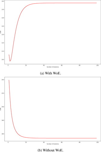
Figure 2(a) shows the Logistic Regression model with WoE that was optimised after approximately 5 iterations. While, Figure 2(b) shows the Logistic Regression model without WoE been optimised after approximately 20 iterations. The estimated Logistic Regression model with and without WoE, respectively, are given as $$\begin{array}{c}Y={\left[1+e^{-(0,0389+0,701X_1+0,434X_2+0,327X_3+0,489X_4+0,437X_5+0,413X_6+0,247X_7+0,336X_8)}\right]}^{-1}\hfill \end{array}$$ and $$\begin{array}{c}Y={\left[1+e^{-(0,017+0,677X_1-0,359X_2+0,245X_3+0,056X_4+0,493X_5+0,356X_6-0,247X_7+0,175X_8)}\right]}^{-1}.\hfill \end{array}$$

Once the coefficients were obtained, the ${\beta }_{\mathit{\text{updated}}}$ values were multiplied by the test feature dataset together with an applied sigmoid function. This was used to get the prediction probability to validate the model. However, a threshold probability was required to be set since the prediction probability is determined for an outcome of 1 (good risk) only. This means that a prediction probability above the threshold probability would mean an outcome equal to 1 (good risk) and below the threshold probability the outcome would be equal to 0 (bad risk). This threshold probability was computed by determining the log loss of the model. For 300 iterations of threshold values, the probability was determined and the log loss was computed using the sklearn.metrics package in Python. This was plotted on a graph to visually see at what threshold value the lowest loss was obtained shown in Figure 3. The log loss is an indicator of how close the prediction probability is to the actual outcome. Hence, the lower the log loss, the better the prediction is.

Figure 3. Log loss for various threshold probabilities for the logistic regression model.

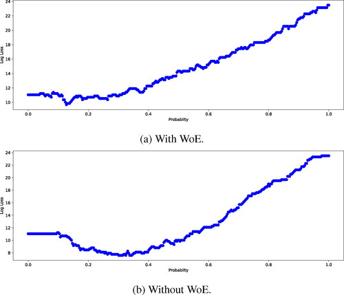
Figure 3(a) shows the threshold probability for the Logistic Regression model with WoE as 0.338 for a log loss of 9.6710. While, Figure 3(b) shows the threshold probability for the Logistic Regression model without WoE is 0.1270 for a log loss of 7.5986.

3.4. Machine learning models

3.4.1. K-Nearest neighbours

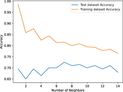
For the K-Nearest Neighbours (KNN) model, the Python sklearn.neighbors package with the KNeighborsClassifier class was used. However, this classifier takes in a specified integer value of neighbours to use when classifying the data. To get the optimal number of neighbours, values from 1 to 15 were used and the accuracy score was evaluated at each iteration. This was plotted visually in Figure 3(a). The graphs show that the accuracy decreased with an increasing number of nearest neighbours. Referring to Figure 4, the best accuracy was determined to be at 7 nearest neighbours and this was the value used in the classification. This optimisation was done for the both the training and test dataset to determine the highest test accuracy traded off with the best training accuracy. It must be noted that a baseline KNN model was used and no hyper-parameter optimisation was determined.

Figure 4. Training and test accuracy of different neighbour values used in the KNN model.

3.4.2. Decision trees

The Python sklearn.tree package with the DecisionTreeClassifier class was used for the Decision Tree model. The Gini Index impurity measure was found to produce the best overall accuracy. The Gini Index was used together with a maximum depth of 4. The maximum depth refers to the level to which the tree is branched down. Furthermore, no hyper-parameter optimisation was used. The structure of the tree revealed that the tree has 4 levels below the highest node. The Gini impurity at each node was determined and the class, 0 or 1, was computed.

3.4.3. Support vector machines

The last machine learning model used was the Support Vector Machines (SVM) model. The Python sklearn.model_selection and sklearn.svm packages together with the GridSearchCV and SVC classes were used for modelling. The SVM classifier in Python takes in three main parameters: C is the regularisation parameter which must be positive and the strength of regularisation is inversely proportional to this parameter, kernel specifies the kernel type to be used in the learning from a list of ‘linear’, ‘poly’, ‘rbf’, ‘signmoid’, ‘precompted’ or a callable predefined function, and lastly gamma is the kernel coefficient if the kernel is ‘rbf’, ‘poly’ or ‘sigmoid’. Then, to determine what combination of these parameters with the correct values, should be used, the GridSearchCV class was used to optimise the parameter set for the best accuracy. The kernel was set as the default of ‘rbf’ because this is the most common and baseline kernel for the SVM algorithm. Initial values for the parameters were set and passed to the GridSearchCV class to optimise. This process took more time than the other machine learning models. The initial parameters values were set as follows: C: (0.01, 0.1, 1, 10, 100, 1000); kernel: ‘rbf’; gamma:(1, 0.1, 0.01, 0.001, 0.0001, 2, 3, 10). After optimising the SVM model, the parameter set for the best overall accuracy was determined to be: ‘C’: 10, ’gamma’: 1, ‘kernel’: ‘rbf’.

3.5. Distribution post feature selection and data balancing

The distribution results for each selected feature after applying the Chi-squared statistics test and data balancing are presented next. For the emphstatus feature, the distribution showed that having more than 200DM or having a salary for at least one year on account, contributed the most to a customer being classified as a good risk. Having no checking account contributed most to a customer being classified as a bad risk. This therefore means that these two categories would hold higher weightings when transforming the data. This is also confirmed by the WoE where category 1 had a WoE of $-0.901$ and category 4 had a WoE of 1.038. The negative sign on the WoE for category occurs from Equation (6)(6) $$\begin{array}{c}\mathit{\text{Wo}}{E}_i=\hspace{0.17em}\mathrm{\text{ln}}\hspace{0.17em}\left(\frac{G_i}{G}÷\frac{B_i}{B}\right),\hfill \end{array}$$(6) where the natural log of a fraction would result in a negative number because the distribution of bad risk would be higher than that of good risk for the category. This category then indicates that the more a person has in his or her checking account, the higher the chance that he or she will be classified as a good risk. This feature was also categorised as the most important in the credit risk dataset according to the Chi-square statistic test with a score of 53.97.

Category 2 for the credit_history feature had the highest distribution for both good and bad risk. This means even after balancing the dataset, a customer would have almost an equal chance of being a bad risk as he or she would be a good risk, if the customer does not have credit history or has already paid back all credits. This is fair since the bank cannot accurately tell if the customer at the current time would be able to pay back the credit or not since there is either no history or no current credit outstanding to assess if the customer is a good or bad risk. Category 4 is the next highly distributed characteristic for the credit_history feature for good and bad risk. However, the customer would have a higher chance of being classified as a good risk if he or she had paid back all credits at the current bank. In other words, the bank knows the customer’s standing and there was some trust built. Category 0 had the highest WoE of $-1.495$ which indicates this category is a good predictor for classifying bad risk. This is expected since a customer having delayed repayments on credit likely means a bad credit risk.

The distribution savings feature shows that category 1 contributed the most to both good and bad risk classification, with bad risk having a higher count. The categories 2, 3 and 4 have similar distribution. Category 1 implies that a person would be classified a bad risk mostly because he or she did not have a savings account. Category 4 had the highest WoE of 1.735 due to the large difference in bad and good risk counts. This would not necessarily mean that the feature was the most important but that in prediction, this category would more than likely mean a customer is a good risk.

For the discretised_duration feature, categories 1, 2 and 3 had the lowest WoE with values of 0.276, $-0.144$ and 0.042, respectively. Category 3 in particular, had a very small WoE because the distribution between good and bad risk were similar. This then meant that these categories would not be good predictors for the model and lower weightings were assigned. However, this can be difficult for the model to predict the correct outcome if the test dataset contain more of these categories. In other words, if the credit duration was between 7 to 24 months, then the customer has roughly an equal chance of being classified a good risk as he or she would be classified a bad risk. Category 0, which meant a credit duration of 0 to 6 months, had a higher distribution of good risk than bad risk. This also meant that the WoE was larger due to the difference. The value for the WoE for this category was 1.981. Categories 4, 5 and 6 also had larger WoE due to the difference in distributions between good and bad risk. An increase in duration would mean that the customer was more likely to be classified as a bad risk.

The property variable consisted of four different categories. Categories 2 and 3 had similar distributions between good and bad risk, therefore, the WoE for each was calculated to be lower. These categories would then not be regarded good classifiers for risk in the dataset. Category 1 and 4 carried the highest WoE of 0.380 and $-0.479,$ respectively. These categories would then be the better risk classifiers in the dataset. The distribution also showed that if a customer owned no property, he or she would more likely be classified as a good risk. On the contrary, if a customer owned a real estate, he or she would more likely be classified a bad risk. However, there are no large gaps in the distributions for categories 1 and 4 and this would make classifying a customer more difficult.

The employment_duration feature shows the distribution amongst the 5 categories. The distribution showed that as the employment duration increases, the likelihood of a customer being classified as a good risk also increased. This is expected since having a longer duration of employment would also mean a customer is able to handle his or her finances better in terms of paying back credit. However, it must be noted that a customer can still be employed for longer but be classified as a bad risk. The distribution showed that categories 4 and 5, had the highest WoE of 0.632 and 0.461, respectively. Categories 1, 2 and 3 have similar WoE and are all negative in value which indicated that the distribution of bad risk was greater than the distribution of good risk in the employment duration of 0 to 4 years.

The discretised_amount variable contained 8 different categories. Categories 0, 1 and 6 had the lowest WoE since the distributions between good and bad risk were similar. Categories 4 and 5 had the highest WoE of $-0.996$ and 1.139, respectively, indicating that these categories are good classifiers for risk in the dataset. The distribution also showed that a credit amount taken of more than 7000DM would likely mean a customer was a bad risk. Categories 2 and 3 had similar WoE of 0.480 and 0.548 which are not high in value but are better classifiers of good risk than bad risk within the dataset. The distributions for this variable indicated that there was no pattern or correlation for identifying whether or not a customer would be classified as a good or bad risk for credit amounts lower than 7000DM.

T discretised_age variable was encoded into 5 categories. This feature does show a pattern in classifying risk within the dataset. The pattern showed that with an increase in age, the likelihood of a customer being classified as good risk also increased. There was also distribution imbalance for all 5 categories between good and bad risk which indicated that this variable would be beneficial to a classification model as there are clearer distinctions between the two target outcomes. The distribution also showed that the highest number of both good and bad risk customers were between the ages of 26 and 35. This category also had the lowest WoE of $-0.269$ and hence it may be more difficult for a model to classify risk if a customer was within this age bracket.

4. Model evaluation

This section will cover the evaluation for the various models after prediction using the test dataset. The test dataset consisted of 136 observations of good risk and 64 observations of bad risk.

The confusion matrix for each model was computed. For the Logistic Regression model with WoE, the matrix shows that there were 127 customers that were correctly predicted as good risks (true positives), while 47 customers were predicted to be good risks but were actually bad risks (false positives or type I error). 17 customers were correctly predicted as bad risks (true negatives), while 9 customers were predicted to be bad risks but were actually good risks (false negatives or type II error). This would then mean that the model’s precision is lower than its recall.

Referring to Table 2, the recall is 93% and the precision is 73%. However, in the current context of identifying risk, it is more important to identify customers as being classified a bad risk than to falsely classify a customer who is a bad risk, as a good risk. Therefore, precision holds more significance than precision for credit risk. Because the Logistic Regression with WoE places emphasis on the weightings of the categories in identifying a risk outcome, the model would have produced a higher recall than precision. On the contrary, identifying customers only as true good risks is not entirely helpful to the bank, and would mean the precision is lower. A good model requires a trade-off between recall and precision. Therefore, the F1 score is used. This is defined as the harmonic mean of precision and recall. For the Logistic Regression with WoE, the F1 score is 82% which indicates the model has a good balance between precision and recall. In other words, the model can accurately capture good risk and correctly classify the risk.

Table 2. Classification scores for all models.

Model	Precision	Recall	F1 score	Jaccard index	Accuracy	AUC	Log loss
Logistic regression with WOE	0.73	0.93	0.82	0.69	0.72	0.60	9.671
Logistic regression	0.85	0.82	0.84	0.72	0.78	0.76	7.599
KNN	0.88	0.69	0.77	0.63	0.73	0.74	–
Decision tree	0.90	0.61	0.73	0.57	0.69	0.73	–
SVM	0.73	0.92	0.81	0.68	0.71	0.59	–

Source: Author's calculations.

For the Logistic Regression without WoE, the matrix shows that there were 112 customers that were correctly predicted as good risks (true positives), while 20 customers were predicted to be good risks but were actually bad risks (false positives or type I error). 44 customers were correctly predicted as bad risks (true negatives), while 24 customers were predicted to be bad risks but were actually good risks (false negatives or type II error). Table 2 shows that this model has similar precision and recall values, 85% and 82%, respectively. Even with the imbalance in the test dataset, the model could detect a particular risk class and correctly classify it. The model gave an overall F1 score of 84% which was 2% higher than the Logistic Regression with WoE model. The recall for the Logistic Regression model with WoE is higher than without WoE. This is because weightings are placed higher for categories which are more relevant to a particular outcome. However, there still exists categories that may have low WoE and these may make up the majority of the observations in the test dataset, rendering the precision of the WoE model lower than the model without WoE. The log loss for the model with WoE was also 2.072 units higher than the model without WoE indicating that the latter model has better performance in predicting credit risk. The Logistic Regression without WoE thus has an overall good performance.

For the KNN model, there were 94 customers that were correctly predicted as good risks (true positives), while 13 customers were predicted to be good risks but were actually bad risks (false positives or type I error). 51 customers were correctly predicted as bad risks (true negatives), while 42 customers were predicted to be bad risks but were actually good risks (false negatives or type II error). This means that the KNN model is better at predicting good risk than bad risk. This may also be due to imbalance in the test dataset as there were more observations of good risk than bad risk and the KNN model can be sensitive to class imbalance since the true performance is based on a balanced training dataset. The precision for the model is much higher than the recall, 88% and 69% respectively, which gives the KNN model fair performance. In terms of banking, the false positives produced should be as low as possible. This is because the cost of defaulting is riskier than the bank not having that risk. However, the recall should not be so low such that the bank does not have many customers taking credit because profits are required to be made. The model produced an F1 score of 77% as shown in Table 2 which is fair in performance for credit risk classification for the dataset.

For the Decision Tree model, there were 83 customers that were correctly predicted as good risks (true positives), while only 9 customers were predicted to be good risks but were actually bad risks (false positives or type I error). 55 customers were correctly predicted as bad risks (true negatives), while 53 customers were predicted to be bad risks but were actually good risks (false negatives or type II error). These values indicate that the model is better at prediction true negatives than true positives and that the precision would be much higher than the recall. This was indeed true referring to Table 2 where the precision is 90% and the recall is only 61%. This model is suitable for identifying bad risk but there was still a large number of false negatives which can be a financial loss for the bank if the bank’s requirement is to have a financial inflow. The overall F1 score was 73% which indicates the model is fair in predicting risk for the particular dataset. For the SVM model, there were 125 customers that were correctly predicted as good risks (true positives), while 47 customers were predicted to be good risks but were actually bad risks (false positives or type I error). 17 customers were correctly predicted as bad risks (true negatives), while 11 customers were predicted to be bad risks but were actually good risks (false negatives or type II error). These values indicate that the model is better at predicting true positives than true negatives and that the recall would be higher than the precision. This was indeed true referring to Table 2 where the precision is 73% and the call is 92%. While this model is suitable for identifying good risk, there was still a large number of false positives which can be a risk for the bank. The overall F1 score was 81% which indicates the model is still good in predicting risk for the particular dataset.

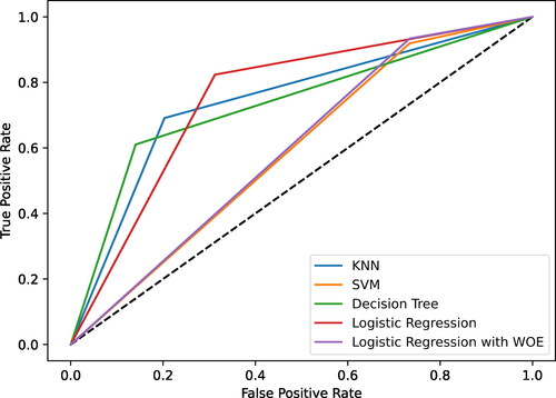
Figure 5 shows the Receiver Operating Characteristic curves for each of the 5 classification models. An ideal curve would be a parallel line to the y-axis connecting to a line parallel to the x-axis. This ideal line would mean the precision and recall are both 100%. In reality, this is not true and can be seen from the various models. The SVM and Logistic Regression with WoE models performed similarly where the models can predict good risk well but suffer from a high number of false positives. These models will then have similar AUC as confirmed from Table 2 with 0.6 and 0.59 for the Logistic Regression with WoE model and SVM model, respectively. These models also have the lowest AUC from all 5 models. The accuracy values and Jaccard Index were also similar. However, these evaluation measures were not strictly used for comparing the models. Because the dataset is imbalanced, the precision, recall and F1 score were the most suitable measures for evaluation. The Decision Tree and KNN models performed similarly AUC values of 0.73 and 0.74, respectively. These models were better at precisely classifying bad risk, however, the models did produce a higher number of false negatives. The Logistic Regression model without WoE performed the best overall from the 5 models. This statistical learning method balanced precision and recall well and produced the highest F1, accuracy, Jaccard Index and AUC values of 84%, 78%, 72% and 76%, respectively. The Receiver Operating Characteristic curve for the model is also bent toward the upper left of the graph which is the closest to the ideal curve.

Figure 5. Receiver operating characteristic curve for all five models.

5. Conclusion

Quantitative learning models can provide banks with the necessary credit assessment by using various statistical and machine learning algorithms that are efficient, economical, and accurate. However, some machine learning models can be computationally demanding and complex. Statistical learning can also provide similar performance with fewer computational resources. This article provided an analytical comparison of 5 models namely the statistical learning models: Logistic Regression with and without transforming features using WoE, and the machine learning models: K-Nearest Neighbours, Decision-Tree, and Support Vector Machines. The analysis of techniques was to understand if the statistical learning models could outperform or perform similarly to the machine learning models. The results showed that not only can the Logistic Regression models perform similarly to the machine learning models but they can outperform the models. The Logistic Regression model without transforming the features performed the best out of the 5 models. Thus, the Logistic Regression model with WoE transformation did not improve the performance of the model. However, this model did perform relatively similarly to the SVM model which required more time and resources to optimise. In the future, the optimal trade-off between precision and recall could be determined so that the models can be accurately and fairly evaluated. This also allows the modeler to determine the suitability of the model for credit risk prediction in commercial banking. Furthermore, the cost of misclassifying a customer’s risk profile could also be determined, while ensuring there is insight information and interpretability of the customer behaviour. Thereby, considering the feasibility and suitability of a Bayesian approach proposed by (Giudici, 2001; Giudici & Raffinetti, 2023; James et al., 2023), in analysing indirect dependencies between predictor variables that make business sense and addressing model uncertainty.

Ethics statement

No animal or human studies involved – all data are non-proprietary and freely available from the internet and other non-proprietary sources.

Data availability statement

The data used in the paper can be provided on request.

Disclosure statement

No potential conflict of interest was reported by the author(s).

Additional information

Funding

The authors received no direct funding for this research.

Notes on contributors

Modisane B. Seitshiro

Modisane Seitshiro completed a PhD in Business Mathematics and Informatics (BMI) at North-West University in 2020. He is currently a Senior Lecturer at the Centre for BMI - NWU. His research interests are Applied Statistics and Quantitative Risk Management.

Seshni Govender

Seshni Govender achieved her Honours BSc in Engineering from the University of the Witwatersrand, Johannesburg, South Africa, in 2019. She also accomplished an Honours BCom degree in Financial Modelling from UNISA in 2022. Currently, she is pursuing a Master of Commerce (MCom) degree in Quantitative Management at UNISA. With a professional journey spanning over 4 years, she has gained valuable experience across diverse sectors including medical and financial administration, banking and consulting. Seshni holds the position of Quantitative Analyst at Nedbank. Her research focus revolves around enhancing the robustness and interpretability of machine learning within the areas of Data Science, Data Engineering and Data Analysis.

References

- Abu Alfeilat, H. A., Hassanat, A. B., Lasassmeh, O., Tarawneh, A. S., Alhasanat, M. B., Eyal Salman, H. S., & Prasath, V S. (2019). Effects of distance measure choice on k-nearest neighbor classifier performance: A review. Big Data, 7(4), 221–248. https://doi.org/10.1089/big.2018.0175
- Aggarwal, A., Kasiviswanathan, S., Xu, Z., Feyisetan, O., & Teissier, N. (2021 Label inference attacks from log-loss scores [Paper presentation]. International Conference on Machine Learning (pp. 120–129). PMLR.
- Awad, M., & Khanna, R. (2015). Support vector machines for classification. In Efficient Learning Machines: Theories, Concepts, and Applications for Engineers and System Designers (pp. 39–66). Apress: Berkeley, CA, USA. https://doi.org/10.1007/978-1-4302-5990-9_3
- Bénédict, G., Koops, V., Odijk, D., & de Rijke, M. (2021). Sigmoidf1: A smooth f1 score surrogate loss for multilabel classification. arXiv preprint arXiv:2108.10566.
- Beniwal, S., & Arora, J. (2012). Classification and feature selection techniques in data mining. International Journal of Engineering Research & Technology (Ijert), 1(6), 1–6.
- Bernardo, J., & Smith, A. (1994). Bayesian theory. Wiley.
- Castelo, R., & Giudici, P. (2001). Association models for web mining. Data Mining and Knowledge Discovery, 5(3), 183–196. https://doi.org/10.1023/A:1011469000311
- Chen, K., Zhu, K., Meng, Y., Yadav, A., & Khan, A. (2020). Mixed credit scoring model of logistic regression and evidence weight in the background of big data. In Intelligent Systems Design and Applications: 18th International Conference on Intelligent Systems Design and Applications (ISDA 2018) held in Vellore, India, December 6–8, 2018 (vol.1, pp. 435–443). Springer.
- Chen, X., Chong, Z., Giudici, P., & Huang, B. (2022). Network centrality effects in peer to peer lending. Physica A: Statistical Mechanics and Its Applications, 600, 127546. https://doi.org/10.1016/j.physa.2022.127546
- Czepiel, S. A. (2002). Maximum likelihood estimation of logistic regression models: Theory and implementation. Available at czep. net/stat/mlelr.pdf, 83.
- De Long, E. R., De Long, D. M., & Clarke-Pearson, D L. (1988). Comparing the areas under two or more correlated receiver operating characteristic curves: A nonparametric approach. Biometrics, 44(3), 837–845.
- Dumitrescu, E. I., Hué, S., Hurlin, C., & Tokpavi, S. (2022). Machine learning for credit scoring: Improving logistic regression with non-linear decision tree effects. European Journal of Operational Research, 297(3), 1178–1192. https://doi.org/10.1016/j.ejor.2021.06.053
- Eelbode, T., Bertels, J., Berman, M., Vandermeulen, D., Maes, F., Bisschops, R., & Blaschko, M B. (2020). Optimization for medical image segmentation: Theory and practice when evaluating with dice score or jaccard index. IEEE Transactions on Medical Imaging, 39(11), 3679–3690. https://doi.org/10.1109/TMI.2020.3002417
- Figini, S., & Giudici, P. (2011). Statistical merging of rating models. Journal of the Operational Research Society, 62(6), 1067–1074. https://doi.org/10.1057/jors.2010.41
- Giudici, P., Hadji-Misheva, B., & Spelta, A. (2020). Network based credit risk models. Quality Engineering, 32(2), 199–211. https://doi.org/10.1080/08982112.2019.1655159
- Giudici, P., & Raffinetti, E. (2023). Safe artificial intelligence in finance. Finance Research Letters, 56, 104088. https://doi.org/10.1016/j.frl.2023.104088
- Giudici, P. S. (2001). Bayesian data mining, with application to benchmarking and credit scoring. Applied Stochastic Models in Business and Industry, 17(1), 69–81. https://doi.org/10.1002/asmb.425
- Groemping, U. (2019). South German credit data: Correcting a widely used data set. Beuth University of Applied Sciences, Berlin, Germany, Technical report 4/2019. http://www1.beuth-hochschule.de/FB_II/reports/Report-2019-004.pdf
- Hand, D. J., & Henley, W E. (1997). Statistical classification methods in consumer credit scoring: A review. Journal of the Royal Statistical Society Series A: Statistics in Society, 160(3), 523–541. https://doi.org/10.1111/j.1467-985X.1997.00078.x
- Henley, W., & Hand, D J. (1996). A k-nearest-neighbour classifier for assessing consumer credit risk. The Statistician, 45(1), 77–95. https://doi.org/10.2307/2348414
- Hull, J., & Suo, W. (2002). A methodology for assessing model risk and its application to the implied volatility function model. The Journal of Financial and Quantitative Analysis, 37(2), 297–318. https://doi.org/10.2307/3595007
- James, G., Witten, D., Hastie, T., Tibshirani, R., & Taylor, J. (2023). Statistical learning. In An introduction to statistical learning: With applications in Python (pp. 15–67). Springer.
- Joseph, V R. (2022). Optimal ratio for data splitting. Statistical Analysis and Data Mining: The ASA Data Science Journal, 15(4), 531–538. https://doi.org/10.1002/sam.11583
- Kaggle. (2020). South german credit prediction. Society for Data Science, BIT Mesra, Kaggle. https://www.kaggle.com/c/south-german-credit-prediction/overview.
- Korkmaz, M., Güney, S., & Yiğiter, Ş. (2012). The importance of logistic regression implementations in the Turkish livestock sector and logistic regression implementations/fields. Harran Tarım ve Gıda Bilimleri Dergisi, 16(2), 25–36.
- Kumar, A., Sharma, S., & Mahdavi, M. (2021). Machine learning (ml) technologies for digital credit scoring in rural finance: A literature review. Risks, 9(11), 192. https://doi.org/10.3390/risks9110192
- Liu, H., Li, J., & Wong, L. (2002). A comparative study on feature selection and classification methods using gene expression profiles and proteomic patterns. Genome Informatics, 13, 51–60.
- Mačerinskienė, I., Ivaškevičiūtė, L., & Railienė, G. (2014). The financial crisis impact on credit risk management in commercial banks. KSI Transactions on Knowledge Society, 7(1), 5–16.
- Muchai, E., & Odongo, L. (2014). Comparison of crisp and fuzzy classification trees using gini index impurity measure on simulated data. European Scientific Journal, 10(18), 130–134.
- Nehrebecka, N. (2018). Predicting the default risk of companies. Comparison of credit scoring models: Logit vs support vector machines. Econometrics, 22(2), 54–73. https://doi.org/10.15611/eada.2018.2.05
- Paryudi, I. (2019). What affects k value selection in k-nearest neighbor. International Journal of Scientific & Technology Research, 8, 86–92.
- Persson, R. (2021). Weight of evidence transformation in credit scoring models: How does it affect the discriminatory power? [PhD thesis]. Lund University.
- Podgorelec, V., Kokol, P., Stiglic, B., & Rozman, I. (2002). Decision trees: An overview and their use in medicine. Journal of Medical Systems, 26(5), 445–463. https://doi.org/10.1023/a:1016409317640
- Satchidananda, S., & Simha, J. B. (2006). Comparing decision trees with logistic regression for credit risk analysis. International Institute of Information Technology.
- Seitshiro, M., & Mashele, H. (2022). Quantification of model risk that is caused by model misspecification. Journal of Applied Statistics, 49(5), 1065–1085. https://doi.org/10.1080/02664763.2020.1849055
- Stanfill, C., & Waltz, D. (1986). Toward memory-based reasoning. Communications of the ACM, 29(12), 1213–1228. https://doi.org/10.1145/7902.7906
- Suhadolnik, N., Ueyama, J., & Da Silva, S. (2023). Machine learning for enhanced credit risk assessment: An empirical approach. Journal of Risk and Financial Management, 16(12), 496. https://doi.org/10.3390/jrfm16120496
- Tu, J V. (1996). Advantages and disadvantages of using artificial neural networks versus logistic regression for predicting medical outcomes. Journal of Clinical Epidemiology, 49(11), 1225–1231. https://doi.org/10.1016/s0895-4356(96)00002-9
- Wang, Y., Zhang, Y., Lu, Y., & Yu, X. (2020). A comparative assessment of credit risk model based on machine learning——A case study of bank loan data. Procedia Computer Science, 174, 141–149. https://doi.org/10.1016/j.procs.2020.06.069
- Weed, D L. (2005). Weight of evidence: A review of concept and methods. Risk Analysis: An Official Publication of the Society for Risk Analysis, 25(6), 1545–1557. https://doi.org/10.1111/j.1539-6924.2005.00699.x
- Xia, Y., Liu, C., Li, Y., & Liu, N. (2017). A boosted decision tree approach using bayesian hyper-parameter optimization for credit scoring. Expert Systems with Applications, 78, 225–241. https://doi.org/10.1016/j.eswa.2017.02.017
- Yang, X., Zhu, Y., Yan, L., & Wang, X. (2015 Credit risk model based on logistic regression and weight of evidence [Paper presentation]. 3rd International Conference on Management Science, Education Technology, Arts, Social Science and Economics (pp. 810–814). Atlantis Press. https://doi.org/10.2991/msetasse-15.2015.180
- Yap, B. W., Ong, S. H., & Husain, N H M. (2011). Using data mining to improve assessment of credit worthiness via credit scoring models. Expert Systems with Applications, 38(10), 13274–13283. https://doi.org/10.1016/j.eswa.2011.04.147
- Zhang, A. (2009). Statistical methods in credit risk modeling [PhD thesis]. University of Michigan.