Panel threshold effect of climate variability on agricultural output in Eastern African countries

Abstract

Recent scientific literature shows that in many developing countries, variability in rainfall and temperature in growing season has detrimental effects on agricultural output, especially when the variability is high. It is yet unclear to what extent or threshold these variations impair the agricultural productivity in some parts of Africa. In this study, we answer this research question using a dynamic panel threshold model on a panel dataset of East African countries for the period 1961–2020. We incorporate climate variables disaggregated into growing and non-growing seasons. The empirical results indicate that growing rainfall variability has significant effects on agricultural output. More specifically, we found a significant negative effect from rainfall variability in spring and summer, when precipitation variability exceeds thresholds of −0.533 mL and −0.902 mL respectively. However, these effects are indistinguishable from zero in fall season. Regarding a growing-season temperature variability, we found no significant effects across seasons. Policy implications are discussed.

Impact statement

The findings suggest that African countries should speed up renovating/investing in small scale technologies to alleviate the impact of the within growing season precipitation variability. To mitigate the effect caused by the growing seasonal variability in precipitation, technologies such as flexible planting, rainwater harvesting, smart water-management systems that use drop-bydrop, sprinkler irrigation processes to improve agricultural output. Furthermore, new policies should be implemented by governments to encourage innovation in technology.

Keywords:

• Adaptation policy
• climate change
• Eastern Africa
• dynamic panel threshold

Reviewing Editor:

• Lanouar Charfeddine, Qatar University, Qatar

Subjects:

• Agriculture and Food
• Environment & Economics
• Development Economics
• Ecological Economics

JEL CODE:

• Q10
• Q18
• Q54

1. Introduction

Climate change affects every aspect of the natural and human ecology, but the most dangerous effects are on the necessities for human survival—food and water. The ability of the agriculture sector to adjust to climate change is a vital component of food security.

East Africa in particular is highly dependent on agriculture. For instance, in Uganda, Ethiopia, Kenya and Tanzania, the agriculture sector represents 24.9%, 40%, 26% (FAO, 2022) and 25.8% respectively of the GDP. This makes these countries being highly vulnerable to any fluctuations in seasonal rainfall amounts. According to the World Bank report (2007), the East Africa is expected to depend on the agricultural sector for decades.

The threats of climate change are certainly a challenge—especially in developing countries, where poverty is a feature that hinders the development. Noy (2009) reveals that following a natural disaster, a developing country faces a much greater decline in gross domestic product than a developed economy would.

To date there is still much confusion about the effect that climate has on agricultural output, particularly in developing countries. Because of this, the impact of climate change on agriculture is increasingly becoming a major area of scientific concern (Huong et al., 2019; Karimi et al., 2018; Lippert et al., 2009; Mendelsohn, 2009, 2014; Molua & Lambi, 2007; Rui-Li & Geng, 2013). For instance, Mendelsohn (2014) investigates the impact of climate change in Asia by employing a Ricardian approach.¹ The findings reveal a small aggregate effect associated with a 1.5 °C warming, but damaging effects of about US$84 billion associated with a 3 °C warming.

However, there is also an increasing concern about climate change variability per season in the agricultural sector (Abbas & Mayo, 2021; Mendelsohn et al., 1994; Victor et al., 1996). For instance, early papers such as Mendelsohn et al. (1994) found that in the US, on average, higher temperatures in all seasons with the exception of autumn reduced farm values, while more rain outside autumn increased farm values.

East Africa region in particular is characterised by substantial weather variability in the main growing season (Abraha-Kahsay & Hansen, 2016; Gebrechorkos et al. 2019, 2020; Ngoma et al., 2023). Growing-season climate variability is crucially important, particularly from a policy perspective, as mitigation is feasible even with small-scale technologies (Conway & Schipper, 2011).

The literature also provides sufficient evidence that climate variables are not linearly related to agricultural outputs (Huong et al., 2019; Mendelsohn, 2014; Mishra & Sahu, 2014; Schlenker & Roberts, 2009; Wang et al., 2009). For instance, Schlenker and and Roberts (2009) investigated the relationship between maize, soybean and cotton yields and temperature in the growing season in the United States, using regression analysis. Their findings revealed that yields increase with temperature up to 29 °C for corn, 30 °C for soybeans, and 32 °C for cotton. But above these thresholds, any further increase in temperature has a negative effect on the agricultural output. They added that the non-linear relationship may be observed on isolation of either time-series or cross-sectional variations in temperature and agricultural-product yields. Furthermore, Huong et al. (2019) added that there is a nonlinear significant relationship between agricultural household revenue and weather variables, as well as inverted U-shaped relationships.²

However, there is one important research question that still remains to be answered: is there a threshold at which climate change or growing-season climate variability produces effects on agricultural output? For policy intervention, it would be appropriate to investigate the threshold at which growing-season rainfall and temperature variability affect agricultural output. We believe that the relationship between climate variability and agricultural output is likely to be non-linear (see Burke, 2015; Huong et al., 2019; Mishra & Sahu, 2014; Schlenker & Roberts, 2009). At some (low) level of variability in rainfall and/or temperature, the relationship could be either positive or neutral (non-existent). At a higher level of climate variability the relationship becomes negative. If such a non-linear relationship exists, then in principle it should be possible to estimate the inflexion point, or the threshold at which the sign of the relationship between the two variables would switch. The possibility of such a non-linear relationship is modelled, for instance, by Wang et al. (2009),³ dealing with agriculture in China. When this threshold exists and is ignored, this may significantly bias the relationship between climate variability and agricultural output.

Traditional panel econometric techniques often employed in applied research, such as Polled Ordinary Least Squares (POLS), Fixed and Random Effects, are all limited in their capacity to answer the research question above. On the other hand, although the application of the traditional instrumental variable regression techniques such as Two-Stage Least Squares (TSLS) and the Generalised Method of Moments (GMM) can be efficient in handling the issue of endogeneity, these are not appropriate for non-linear models. Hansen (1999) introduced an econometric framework which allows the investigation of the relationship between two or more variables, if and only if the expected relationship is hypothesised to be non-linear. Nevertheless, the Hansen (1999) model also presents limitations, and one of them is the issue of strict exogeneity of the regressors. In agricultural economics, it has been shown that if there is more capital in the form of livestock⁴ (as is the case in Eastern Africa), it is plausible that more output could be produced. The higher the level of output, the higher the investment ratio of capital is likely to be (FAO, 2008). Hence a causal relationship is possible between capital investment and agricultural output. For this reason, we reinvestigate the econometric effects of climate variability on agricultural output in Eastern Africa, using a dynamic version of the Hansen model. We aim to shed more light on the effects of growing-season variability in rainfall and temperature on agricultural output. We seek to determine whether there is a turning point (a threshold) at which climate variability impacts agricultural output. To the best of our knowledge, this is the first study to answer this specific research question.

The estimation results reveal that the growing season rainfall variability has an impact mainly in the major growing seasons. Lag output is significant across all specifications, meaning last period agricultural harvest is important to the current agricultural harvest. In the context of the rural economy that characterises Eastern Africa, the livelihoods of farmers depend on their choice of how to allocate resources to generate the highest income possible, given the constraints they are facing. These decisions depend on the income generated by farmers, making lag output one of the most important features in decision making. After controlling for endogeneity, the results reveal that growing season rainfall variability negatively affects agricultural output; however, there is no significant evidence for the effect of growing season temperature variability in the major season. After using the dynamic panel threshold estimation, we found that the threshold for growing season rainfall in spring is −0.553 in spring, −0.902 in summer, and 1.261 in the fall season. In the case of growing season temperature variability, we found no significant effects.

The rest of the paper is organised as follows. Section 2 is a brief review of the existing literature. Section 3 presents the model specification, and Section 4 describes the data and variables. Section 5 presents the results, and Section 6 concludes.

2. Literature review

According to Scholes and Biggs, climate change poses significant risks to development, especially in sub-Saharan Africa. In addition to being undeniably warming, it is becoming more and more evident that human activity is mostly to blame for the majority of the warming that has happened over the past 50 years (Intergovernmental Panel on Climate Change [IPCC], 2007).

Consequently, all continents and in most seas are experiencing substantial changes in their physical and biological systems (ConsTable et al., 2014).

Research organizations, development agencies, and governments are working hard to find answers to these and other related problems. These include what the effects could be on agricultural systems and food security, as well as what alternatives families in vulnerable regions have for adapting.

However, there are still significant gaps in our understanding of the various and interrelated pressures that affect the vulnerability of Africa’s impoverished.

East Africa’s economy particular, is highly dependent on agriculture, which generates 40% of the gross domestic product and is the main source of income (up to 80%) (Runge et al., 2004). Because of this dependency, the most important threat to agricultural production is the growing season weather variability documented in the literature in general (Owusu & Waylen, 2013; Rosenzweig et al., 2007; Victor et al., 1996) and in East Africa in particular (Bahaga et al., 2014; Conway et al., 2005; Conway & Schipper, 2011; Schreck & Semazzi, 2004; You et al., 2009). Regan et al. (2019) suggested for instance, that food yields worldwide have decreased by up to 10% as a result of weather variability related events but the consequences differ as a function of the heterogeneity across countries. A large portion of this adaptive capacity variation comes from governmental decisions about structural readiness. In addition, according to Chandio et al. (2020)’s findings, temperature and rainfall have a negative long-term impact on agricultural productivity, whereas CO₂ emissions have a substantial short- and long-term impact on agricultural output.

Numerous studies have estimated the effects of climate change by using production functions in which different proxies are employed for climate change and climate change variability (Barrios et al., 2008; Blanc, 2012; Lobell & Burke, 2010; Rowhani et al., 2011; Schenker & Lobell, 2010; Ward et al., 2014). Different climate variables such as annual and seasonal growing temperature and precipitation (Ward et al., 2014) have been used as proxies for climate variation in these estimations. Other climate variables have also been considered, such as evapotranspiration, standardised precipitation index (Gebrechorkos et al., 2020), drought and floods (Blanc, 2012); temperature and precipitation variance (Rowhani et al., 2011), coefficient of variation (Abraha-Kahsay & Hansen, 2016), and Standardized Precipitation Evapotranspiration Index (SPEI).

The importance of growing season climate variability and its inclusion in the production function has been documented around the world as well. For instance, Cabas et al. (2009) found that increases in both temperature and rainfall variability harm crop production in Nepal and Canada, while temperature variability has been found to have a negative effect on key crops in the US (McCarl et al., 2008). Changes in mean and growing season temperature and rainfall induce heterogeneous impacts, which can be regarded as harmful, beneficial or even negligible, depending on altitude and type of crop (Poudel & Kotani, 2013).

In Africa, and specifically East Africa, studies (Abraha-Kahsay & Hansen, 2016; Ward et al., 2014) have shown that growing season climate variability has an effect on agricultural output. For instance, Ward et al. (2014) used three estimation techniques (OLS, non-spatial and spacial Heckit models) to assess the impact of growing season variability on aggregate cereal yield in sub-Saharan Africa. They found that in growing season, precipitation variability has a positive impact on agricultural outputs. Abraha-Kahsay and Hansen (2016) employed fixed effect estimation to determine whether growing season variability has an effect on agricultural yield in East Africa. They disaggregated the annual climate variables, to distinguish between two seasons (growing and non-growing), and found a substantial negative impact from growing season variability in rainfall. Rowhani et al. (2011) also found that growing season precipitation variability has a negative effect on agricultural outputs in East Africa. On the other hand, Barrios et al. (2008) found growing season variation in precipitation to be insignificant.

Recently, Chandio et al. (2022), Toret et al. (2022), Pickson et al. (2022), Lachaud et al. (2022), Nguyen and Scrimgeour (2022) investigated the impact of climate change on the agricultural product. For instance, Nguyen and Scrimgeour (2022) examined the economic effects of climate changes on Vietnamese agriculture. The Ricardian model’s panel evidence points to seasonal and regional variations in the effects of the climate on the agricultural product. With the exception of spring time temperatures and rising seasonal temperatures are generally linked to losses. While precipitation accumulations in the summer season are beneficial for reducing the consequences of temperature rise

In Africa, in East Africa in particular, some studies like Bedeke (2023), Mubenga-Tshitaka et al. (2023), Espoir et al. (2022), Pickson et al. (2022), Warsame et al. (2021), Abdi et al. (2022) have investigated as well the impact of climate change on the agriculture sector. For instance, Abdi et al. (2022) examined the impact of climate change on the production of cereal crops in nine East African countries for period between 1990 and 2018. The findings demonstrate that rainfall and carbon emissions have positive and significant long-term effects on cereal crop production. For long-term food security, there must be a political commitment to reducing the harm of the impact of burning fossil fuels of the global climate (Anderson et al. 2020).

Most of these studies that have focused on the impact of growing season variability in rainfall have relied on fixed effect models (Abraha-Kahsay & Hansen, 2016; Barrios et al., 2008; Lobell et al., 2011; Ward et al., 2014), and some like (Abdi et al., 2022; Espoir et al 2022) replied on the average effect of climate variables on the agriculture output. These studies assume that there is a linear relationship between agricultural output and climate variables, or variability in climate variables. In addition, these studies did not consider the effect of rain fall and temperature in a particular session. Our research sheds light on the non-linear relationship between these, and the threshold below or above which such a relationship becomes harmful to agricultural output. Few studies like Chen and Gong (2021) considered the non-linear relationship as well but concentrated on the total factor productivity and climate change nexus and determined a threshold, not on the climate change variability per season and the agricultural output.

3. Model specification

3.1. Model 1: standard production function

In the standard production function, the dependent variable (agricultural output) is regressed with inputs expressed as follows: (1) $$Q=F(L,K,\mathrm{{\rm I}})$$(1)

Where $Q$ stands for agriculture output, L for labour, K for capital (such as land, machinery and livestock), and $\mathrm{{\rm I}}$ refers to other factors such as fertiliser and irrigation. We assume a Cobb-Douglas production function as in Abraha-Kahsay and Hansen (2016), expressed as follows: (2) $$Q=L^{{\beta }_1}{K}^{{\beta }_2}{\mathrm{{\rm I}}}^{{\beta }_3}$$(2)

Taking into account the dynamic nature of agriculture, the standard model can be expressed as follows: (3) $$\mathit{\text{ln}}\left({\mathit{\text{Output}}}_{\mathit{\text{it}}}\right)={\beta }_0+{\beta }_1\mathit{\text{ln}}\left({\mathit{\text{Output}}}_{\mathit{\text{it}}-1}\right)+{\beta }_2\mathrm{\text{ln}}\hspace{0.17em}\left({\mathit{\text{Labour}}}_{\mathit{\text{it}}}\right)+{\beta }_3\mathrm{\text{ln}}\hspace{0.17em}\left({\mathit{\text{Land}}}_{\mathit{\text{it}}}\right)+{\beta }_4\mathrm{\text{ln}}\hspace{0.17em}\left({\mathit{\text{Machinery}}}_{\mathit{\text{it}}}\right)+{\beta }_5\mathrm{\text{ln}}\hspace{0.17em}\left({\mathit{\text{Livestock}}}_{\mathit{\text{it}}}\right)+{\beta }_6\mathrm{\text{ln}}\hspace{0.17em}\left({\mathit{\text{Fertiliser}}}_{\mathit{\text{it}}}\right)+{{\beta }_7\mathit{\text{ln}}(\mathit{\text{Irrigation}}}_{\mathit{\text{it}}})+\sum _{n=1}^3{\alpha }_{1s}\mathrm{\text{ln}}\hspace{0.17em}\left({\mathit{\text{Temp}}}_{\mathit{\text{ist}}}\right)+\sum _{n=1}^3{\alpha }_{2s}\mathrm{\text{ln}}\hspace{0.17em}\left({\mathit{\text{Precip}}}_{\mathit{\text{ist}}}\right)+\sum _{n=1}^3{\lambda }_{1s}\mathrm{l}\mathrm{n}\left({\mathit{\text{Variability}}}_{\mathit{\text{ist}}}^{\mathit{\text{Temp}}}\right)+\sum _{n=1}^3{\lambda }_{2s}\mathrm{\text{ln}}\hspace{0.17em}\left({\mathit{\text{Variability}}}_{\mathit{\text{ist}}}^{\mathit{\text{Rainfall}}}\right)+{\rho \mathit{\text{TT}}}_{\mathit{\text{it}}\mathrm{ }}+{\mathit{\mu }}_i+{\epsilon }_{\mathit{\text{it}}}$$(3)

Where ${\mathit{\text{Output}}}_{\mathit{\text{it}}}$ and ${\mathit{\text{Output}}}_{\mathit{\text{it}}-1}$ are the total agricultural production of the country, and the lag of the total agricultural production is i (i = 1,2,$\cdots n$) in year t(t = 1,2$,\dots ,T$), and ${\epsilon }_{\mathit{\text{it}}}$ the error. We include three capital inputs: Land, Machinery and Livestock. We also include Labour, Fertiliser and irrigation; ${\mathit{\mu }}_i$ is the unobserved time-invariant country-specific effect, ${\mathit{\text{TT}}}_{\mathit{\text{it}} }$ is the country-specific time trend, and ${\epsilon }_{\mathit{\text{it}}}$ is the error term. We follow Barrios et al. (2008), Molua (2008) and Abraha-Kahsay and Hansen (2016) in specifying the augmented agriculture production function. ${\mathit{\text{Temp}}}_{\mathit{\text{ist}}}$ and ${\mathit{\text{Rainfall}}}_{\mathit{\text{ist}}}$ are the mean temperature and rainfall for country i in season s (s = 1,2,$\cdots ,S$) in year t. Likewise, ${\mathit{\text{Variability}}}_{\mathit{\text{ist}}}^{\mathit{\text{Temp}}}$ and ${\mathit{\text{Variability}}}_{\mathit{\text{ist}}}^{\mathit{\text{Rainfall}}}$ are growing season temperature and rainfall variability.

In this study, the empirical analysis was performed using System Generalized Method of Moments (GMM) estimator proposed by Arellano and Bover (1995) and Blundell and Bond (1998). The System GMM estimator is used in the panel data methodological framework presents some advantages. First, given the dynamic panel data framework, the alternatives—Ordinary Least Squares (OLS) levels and Within Group estimators—produce biased and inconsistent estimates as the unobserved time invariant country effects are not included. Second, the System GMM estimator produces reliable and efficient parameter estimates for regressions in which the regressors are correlated with both past and present realizations of the error and/or exhibit heteroscedasticity and autocorrelation among individuals (Roodman, 2009). Thirdly, the System GMM estimator not only removes dynamic panel bias but also resolves the problems of fixed effects and regressor endogeneity (Nickell, 1981). The lagged dependent variable and other endogenous factors are instrumented using variables uncorrelated with the fixed effects to control the endogeneity of regressors.

3.2. Model 2: panel threshold model

We follow Kremer et al. (2013) in establishing a dynamic panel threshold model for the agricultural production function. The Kremer et al. (2013) model is an extension of the static panel threshold model proposed by Hansen (1999) and the cross-section threshold regression of Caner and Hansen. The dynamic panel threshold accounts for non-linearities and endogeneity bias in the model, as it is built on the GMM that solves the endogeneity. Indeed, in this study we analyse the role of the growing seasonal variability in temperature and rainfall threshold in the relationship between agricultural output, climate variability and the endogenous regressor (lagged of the output). The expression for the dynamic panel threshold model is written as follows: (4) $$\mathrm{\text{ln}}\hspace{0.17em}\left({\mathit{\text{Output}}}_{\mathit{\text{it}}}\right)=u_i+{\beta }_1{\tilde{\pi }}_{\mathit{\text{it}}}I\left({\tilde{\pi }}_{\mathit{\text{it}}}\le \gamma \right)+{\delta }_{1}I\left({\tilde{\pi }}_{\mathit{\text{it}}}\le \gamma \right)+{\beta }_2{\tilde{\pi }}_{\mathit{\text{it}}}I\left({\tilde{\pi }}_{\mathit{\text{it}}}>\gamma \right)+{\mathit{\varphi }Z}_{\mathit{\text{it}}}+{\epsilon }_{\mathit{\text{it}}}$$(4)

Where the subscripts $i=1,···,N$ and $t=1,···,T$ represent the country and time index respectively. $I(\bullet )$ is the indicator function and the threshold $\gamma .$ $u_i$ is the country-specific fixed effect while ${\epsilon }_{\mathit{\text{it}}}$ is the error term, ${\epsilon }_{\mathit{\text{it}}}\sim \mathit{\text{iid}}(0,{\sigma }^2).$ ${\tilde{\pi }}_{\mathit{\text{it}}}$ (growing season variability) represents the threshold and the regime dependent regressor. $Z_{\mathit{\text{it}}}$ represents the vector of endogenous variables where the estimated slope coefficients are regime independent. $\mathit{\text{ln}}({\mathit{\text{Output}}}_{\mathit{\text{it}}}),$ the log output is the dependent variable. $Z_{\mathit{\text{it}}}$ represents the m-dimensional vector of explanatory regressors that might include the lagged output, while $Z_{1\mathit{\text{it}}}$ captures the other control variables. The coefficient ${\delta }_1$ is the regime intercept. ${\beta }_{1 }$ represents the marginal impact of growing seasonal variability in rainfall and temperature on agricultural output in the long run when the variability is below the threshold, while ${\beta }_{2 }$ captures the marginal impact of growing seasonal variability in rainfall and temperature above the threshold. The ${\beta }_i$ coefficients are obtained by GMM estimation. According to Arellano and Bover (1995), the lags of the dependent variables (endogenous variables) ${\mathit{\text{Output}}}_{\mathit{\text{it}}-2}\cdots {\mathit{\text{Output}}}_{\mathit{\text{it}}-k}$ are used as instruments. Arellano and Bover (1995) confirmed that error terms are not auto-correlated, and the cross-section threshold of Caner and Hansen (2004) applies to the dynamic panel approach. Thus, the individual fixed effects are eliminated by the forward orthogonal deviation transformation.

The forward orthogonal deviation transformation for the error term can be expressed as (5) $${\epsilon }_{\mathit{\text{it}}}^{\mathrm{*}}=\sqrt{\frac{T-t}{T-t+1}}\left[{\epsilon }_{\mathit{\text{it}}}-\frac{1}{T-t}({\epsilon }_i(t+1)+\cdots +{\epsilon }_{\mathit{\text{iT}}}\right]$$(5)

The error terms of the forward orthogonal transformation remain homoscedastic; that is, (6) $$\mathit{\text{Var}}\left({\epsilon }_i\right)={\sigma }^2{I}_T⟹\mathit{\text{Var}}\left({\epsilon }_i\right)={\sigma }^2{I}_{T-1}$$(6)

According to Kremer et al. (2013), firstly the endogenous variable $Z_{2\mathit{\text{it}}}$ is estimated as a function of the instrument $X_{\mathit{\text{it}}}$ and we obtain the predicted value ${\widehat{Z}}_{2\mathit{\text{it}}}.$ Secondly, Equation (4)(4) $$\mathrm{\text{ln}}\hspace{0.17em}\left({\mathit{\text{Output}}}_{\mathit{\text{it}}}\right)=u_i+{\beta }_1{\tilde{\pi }}_{\mathit{\text{it}}}I\left({\tilde{\pi }}_{\mathit{\text{it}}}\le \gamma \right)+{\delta }_{1}I\left({\tilde{\pi }}_{\mathit{\text{it}}}\le \gamma \right)+{\beta }_2{\tilde{\pi }}_{\mathit{\text{it}}}I\left({\tilde{\pi }}_{\mathit{\text{it}}}>\gamma \right)+{\mathit{\varphi }Z}_{\mathit{\text{it}}}+{\epsilon }_{\mathit{\text{it}}}$$(4) above is estimated by ordinary least squares, after substituting $Z_{2\mathit{\text{it}}}$ for the predicted value ${\widehat{Z}}_{2\mathit{\text{it}}}.$ The residual sum of squares from the equation is noted as $S(\gamma ),$ where $\gamma$ denotes the common threshold value to be estimated. The optimal value of the threshold estimated $\widehat{\gamma }$ is such that the residual sum of squares is minimised as $\widehat{\gamma }={\mathrm{\text{arg}}\mathrm{\text{min}}}_{\gamma }{S}_n(\gamma ).$ Thirdly, after obtaining $\widehat{\gamma },$ the estimated threshold value, the regression slope coefficients are found by GMM using the instruments and the estimated threshold $\mathrm{ }\widehat{\gamma }.$ The 95% critical values for determining the confidence interval of the threshold value are expressed as $\mathrm{\Gamma }=\left\{\gamma :\mathit{\text{LR}}(\gamma )\le C(\alpha )\right\},$ where $C(\alpha )$ is the 95% percentile of the asymptotic distribution of the likelihood ratio $\mathit{\text{LR}}(\gamma ).$

Given the nature of Equation (3)(3) $$\mathit{\text{ln}}\left({\mathit{\text{Output}}}_{\mathit{\text{it}}}\right)={\beta }_0+{\beta }_1\mathit{\text{ln}}\left({\mathit{\text{Output}}}_{\mathit{\text{it}}-1}\right)+{\beta }_2\mathrm{\text{ln}}\hspace{0.17em}\left({\mathit{\text{Labour}}}_{\mathit{\text{it}}}\right)+{\beta }_3\mathrm{\text{ln}}\hspace{0.17em}\left({\mathit{\text{Land}}}_{\mathit{\text{it}}}\right)+{\beta }_4\mathrm{\text{ln}}\hspace{0.17em}\left({\mathit{\text{Machinery}}}_{\mathit{\text{it}}}\right)+{\beta }_5\mathrm{\text{ln}}\hspace{0.17em}\left({\mathit{\text{Livestock}}}_{\mathit{\text{it}}}\right)+{\beta }_6\mathrm{\text{ln}}\hspace{0.17em}\left({\mathit{\text{Fertiliser}}}_{\mathit{\text{it}}}\right)+{{\beta }_7\mathit{\text{ln}}(\mathit{\text{Irrigation}}}_{\mathit{\text{it}}})+\sum _{n=1}^3{\alpha }_{1s}\mathrm{\text{ln}}\hspace{0.17em}\left({\mathit{\text{Temp}}}_{\mathit{\text{ist}}}\right)+\sum _{n=1}^3{\alpha }_{2s}\mathrm{\text{ln}}\hspace{0.17em}\left({\mathit{\text{Precip}}}_{\mathit{\text{ist}}}\right)+\sum _{n=1}^3{\lambda }_{1s}\mathrm{l}\mathrm{n}\left({\mathit{\text{Variability}}}_{\mathit{\text{ist}}}^{\mathit{\text{Temp}}}\right)+\sum _{n=1}^3{\lambda }_{2s}\mathrm{\text{ln}}\hspace{0.17em}\left({\mathit{\text{Variability}}}_{\mathit{\text{ist}}}^{\mathit{\text{Rainfall}}}\right)+{\rho \mathit{\text{TT}}}_{\mathit{\text{it}}\mathrm{ }}+{\mathit{\mu }}_i+{\epsilon }_{\mathit{\text{it}}}$$(3) above, and as emphasised in the introduction, one might argue that the relationship between growing season variability and agricultural output may not be linear. It has also been argued that the threshold model can be appropriate for consistently and efficiently capturing the overall effect between the variables.

4. Description of data and variables

We constructed a panel of nine countries (Burundi, Djibouti, Ethiopia, Kenya, Rwanda, Somalia, Sudan, Tanzania and Uganda) covering the period from 1961 to 2020 annually data. As in Abraha-Kahsay and Hansen (2016), the nine countries were chosen due to their similar crop production season characteristics. Data points were sourced from FAOSTAT.

The FAO’ net production index has been used as a dependent variable. It is considered a proxy for total production output and includes both crop and livestock production as well as other agricultural outputs. Land input is a proxy for total area used for agricultural purposes, while machinery input is a proxy for total number of tractors used. For livestock capital input, we use the headcount for cattle, sheep and goats. Labour is proxied by the population fraction active in the agriculture sector. Fertiliser input is the number of metric tonnes of plant nutrients consumed in the agriculture sector, while irrigation input is the agricultural area under irrigation. Our definition and inclusion of these variables follows the example of numerous studies (e.g. Abraha-Kahsay & Hansen, 2016; Antle, 1983; Hayami & Ruttan, 1970).

We also follow Ward et al. (2014) and Abraha-Kahsay and Hansen (2016) in the treatment of irrigation as indicator of the quality of land capital input. We use the Climate Research Unit (CRU) as the main source of climate data, as did Barrios et al. (2008) and Abraha-Kahsay and Hansen (2016). As in Abraha-Kahsay and Hansen (2016), ${\mathit{\text{Temp}}}_{\mathit{\text{Springs}}},$ ${\mathit{\text{Temp}}}_{\mathit{\text{Summer}}},$ ${\mathit{\text{Temp}}}_{\mathit{\text{Fall}}},$ ${\mathit{\text{Rainfall}}}_{\mathit{\text{Spring}}},$ ${\mathit{\text{Rainfall}}}_{\mathit{\text{Summer}}}$ and ${\mathit{\text{Rainfall}}}_{\mathit{\text{Fall}}}$ represent the mean temperature and rainfall during spring, summer and fall seasons respectively; while ${\mathit{\text{Variability}}}_{\mathit{\text{Springs}}}^{\mathit{\text{Temp}}},$ ${\mathit{\text{Variability}}}_{\mathit{\text{Summer}}}^{\mathit{\text{Temp}}},$ ${\mathit{\text{Variability}} }_{\mathit{\text{Fall}}}^{\mathit{\text{Temp}}},$ ${\mathit{\text{Variability}}}_{\mathit{\text{Spring}}}^{\mathit{\text{Rainfall}}},$ ${\mathit{\text{Variability}}}_{\mathit{\text{Summer}}}^{\mathit{\text{Rainfall}}}$ and ${\mathit{\text{Variability}}}_{\mathit{\text{Fall}}}^{\mathit{\text{Rainfall}}}$ 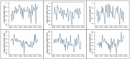represent growing season temperature and rainfall during spring, summer and fall season respectively. Spring season includes the month of March, April and May; fall comprises the month of September, October and December, while the summer contains the month of June, July and August (Abraha-Kahsay & Hansen, 2016). Seasonal variability in temperature and rainfall follow the definition from Amare et al. (2018). We measure variability as the deviation of the previous year’s rainfall and temperature during spring, summer and fall from the 30-year historical average during crop growing seasons (spring, summer and fall). Variability is also referred to as rainfall and temperature anomalies. We also add the growing summer season, as in Abraha-Kahsay and Hansen (2016); apart from spring and fall, the major and minor crop-growing seasons, the summer season can be crucial to the growth and maturity of crops planted in spring. Figure 1 below shows the general trends in rainfall and temperature during the three growing seasons. In general, average growing season variability in rainfall is more significant in all three seasons. There is a trend of gradual decline; spring and fall (the major and minor growing seasons) are more volatile than summer. This has a serious effect on the growth of crops, and is generally characterised by a decreasing trend, while temperature shows an increasing trend, in line with what has been reported in the literature (IPCC, 2007).

Figure 1. Average seasonal variability in rainfall and temperature.

5. Estimation results

We investigate whether the series is stationary. To check the stationary in our panel, we use the Levin et al. (2002) panel unit root test and the Fisher type, based on the augmented Dickey-Fuller tests (Choi, 2001) (see Appendix, Table A3). Both tests reject the null hypothesis at level that the panel contains a unit root. We test the presence of serial correlation using the Wald test, following Wooldridge (2002), in which it was rejected.

Table A4 in the Appendix shows the estimation results of the fixed-effect model. The coefficients of the physical inputs vary slightly when one moves across all the specifications, and they do have the expected signs. Livestock and labour parameters are positive and significant across all the specifications, in line with the literature. Machinery and irrigation coefficients are insignificant, confirming the lack of such tools in the process of agricultural production. East Africa is dominated by traditional practices, mainly based on human muscle power (FAO, 2008). Up to 95% of agriculture there is characterised by traditional small scale non-mechanised practices (FAOSTAT, 2011). The land is the most important factor, with coefficients that have the expected sign and significant. An increase of 1% in the size agricultural land areas is substantially higher compared to coefficients of other regressors. These findings are consistent with the literature (Abraha-Kahsay & Hansen, 2016; Barrios et al., 2008).

Concerning climate variables, the mean effect of rainfall and temperature on the agricultural output during the major growing season (spring) is positive and significant. The major season is characterised by heavy and prolonged rain, but also associated with higher temperature. This favours evaporation, reducing the impact of heavy rain on agricultural output.

During the minor growing season (fall), the coefficients of temperature and rainfall are negative and significant, consistent with expectations. The results for the summer growing season show that the higher temperature affects agricultural output negatively. According to Niang et al. (2014), temperatures in Africa are projected to rise much faster than in the rest of the world; the increase is expected to exceed 2 °C by the twenty-first century, and could reach 4 °C by the end of the twenty-first century. As temperatures rise, agriculture will move to higher latitudes, where soils and nutrients are less suited to crop cultivation (Gomez-Zavaglia et al. 2020).

The growing season rainfall variability of spring has a negative impact on output and the impact tends to persist, even during summer. In line with Conway et al. (2005) who noticed that Eastern Africa has two rainfall regimes that bring rain, from March to May and from October to December, but with great inter-annual variability. Growing season temperature variability had a positive impact during spring (the major growing season), contrary to the results of Abraha-Kahsay and Hansen (2016), who found its effect to be positive and insignificant. It had no effect in summer and fall.

These findings are crucial, given East Africa’s rain-fed nature. Growing season rainfall and temperature variability can have a significant impact on output, even if there are no changes observed at the mean temperature and rainfall level. Our results are consistent with the literature on the effect of variability in rainfall and temperature on agricultural crops in East Africa (Abraha-Kahsay & Hansen, 2016; Barrios et al., 2008; Blanc, 2012; Rowhani et al., 2011; Ward et al., 2014). The majority of these studies found that precipitation variability has a positive effect and temperature variability has a negative impact. For instance, Abraha-Kahsay and Hansen (2016) and Rowhani et al. (2011) both found growing season precipitation variability had a substantial negative effect on output, while Ward et al. (2014) found a positive effect. This is partly in line with our findings, which state that growing season rainfall variability has a negative effect, but growing season temperature variability has a positive significant effect as well.

Table 1 below shows the results of the dynamic GMM using Equation (3)(3) $$\mathit{\text{ln}}\left({\mathit{\text{Output}}}_{\mathit{\text{it}}}\right)={\beta }_0+{\beta }_1\mathit{\text{ln}}\left({\mathit{\text{Output}}}_{\mathit{\text{it}}-1}\right)+{\beta }_2\mathrm{\text{ln}}\hspace{0.17em}\left({\mathit{\text{Labour}}}_{\mathit{\text{it}}}\right)+{\beta }_3\mathrm{\text{ln}}\hspace{0.17em}\left({\mathit{\text{Land}}}_{\mathit{\text{it}}}\right)+{\beta }_4\mathrm{\text{ln}}\hspace{0.17em}\left({\mathit{\text{Machinery}}}_{\mathit{\text{it}}}\right)+{\beta }_5\mathrm{\text{ln}}\hspace{0.17em}\left({\mathit{\text{Livestock}}}_{\mathit{\text{it}}}\right)+{\beta }_6\mathrm{\text{ln}}\hspace{0.17em}\left({\mathit{\text{Fertiliser}}}_{\mathit{\text{it}}}\right)+{{\beta }_7\mathit{\text{ln}}(\mathit{\text{Irrigation}}}_{\mathit{\text{it}}})+\sum _{n=1}^3{\alpha }_{1s}\mathrm{\text{ln}}\hspace{0.17em}\left({\mathit{\text{Temp}}}_{\mathit{\text{ist}}}\right)+\sum _{n=1}^3{\alpha }_{2s}\mathrm{\text{ln}}\hspace{0.17em}\left({\mathit{\text{Precip}}}_{\mathit{\text{ist}}}\right)+\sum _{n=1}^3{\lambda }_{1s}\mathrm{l}\mathrm{n}\left({\mathit{\text{Variability}}}_{\mathit{\text{ist}}}^{\mathit{\text{Temp}}}\right)+\sum _{n=1}^3{\lambda }_{2s}\mathrm{\text{ln}}\hspace{0.17em}\left({\mathit{\text{Variability}}}_{\mathit{\text{ist}}}^{\mathit{\text{Rainfall}}}\right)+{\rho \mathit{\text{TT}}}_{\mathit{\text{it}}\mathrm{ }}+{\mathit{\mu }}_i+{\epsilon }_{\mathit{\text{it}}}$$(3) above. The fixed effect estimations and even the random effect estimations are subject to some shortcomings. They have the problem of potential endogeneity of regressors, as well as a loss of dynamic information. We include in Equation (3)(3) $$\mathit{\text{ln}}\left({\mathit{\text{Output}}}_{\mathit{\text{it}}}\right)={\beta }_0+{\beta }_1\mathit{\text{ln}}\left({\mathit{\text{Output}}}_{\mathit{\text{it}}-1}\right)+{\beta }_2\mathrm{\text{ln}}\hspace{0.17em}\left({\mathit{\text{Labour}}}_{\mathit{\text{it}}}\right)+{\beta }_3\mathrm{\text{ln}}\hspace{0.17em}\left({\mathit{\text{Land}}}_{\mathit{\text{it}}}\right)+{\beta }_4\mathrm{\text{ln}}\hspace{0.17em}\left({\mathit{\text{Machinery}}}_{\mathit{\text{it}}}\right)+{\beta }_5\mathrm{\text{ln}}\hspace{0.17em}\left({\mathit{\text{Livestock}}}_{\mathit{\text{it}}}\right)+{\beta }_6\mathrm{\text{ln}}\hspace{0.17em}\left({\mathit{\text{Fertiliser}}}_{\mathit{\text{it}}}\right)+{{\beta }_7\mathit{\text{ln}}(\mathit{\text{Irrigation}}}_{\mathit{\text{it}}})+\sum _{n=1}^3{\alpha }_{1s}\mathrm{\text{ln}}\hspace{0.17em}\left({\mathit{\text{Temp}}}_{\mathit{\text{ist}}}\right)+\sum _{n=1}^3{\alpha }_{2s}\mathrm{\text{ln}}\hspace{0.17em}\left({\mathit{\text{Precip}}}_{\mathit{\text{ist}}}\right)+\sum _{n=1}^3{\lambda }_{1s}\mathrm{l}\mathrm{n}\left({\mathit{\text{Variability}}}_{\mathit{\text{ist}}}^{\mathit{\text{Temp}}}\right)+\sum _{n=1}^3{\lambda }_{2s}\mathrm{\text{ln}}\hspace{0.17em}\left({\mathit{\text{Variability}}}_{\mathit{\text{ist}}}^{\mathit{\text{Rainfall}}}\right)+{\rho \mathit{\text{TT}}}_{\mathit{\text{it}}\mathrm{ }}+{\mathit{\mu }}_i+{\epsilon }_{\mathit{\text{it}}}$$(3) , among other things, the lagged variable of agricultural output. The lag of output is significant across all specifications. This implies that the decision to engage in agriculture practices depends heavily on what the last agricultural outcome was. Agriculture in general involves many decisions: what and how much to sell to generate cash, which inputs to use, how and when to use them, how much to store if there is an expectation of more favourable conditions in the market, or in the next agriculture season. Also, small household farmers make these decisions in a market that does not function well. This implies that good agricultural results in the previous season can solve a substantial portion of these questions, and will have significant implications for their choices and livelihoods. Hence, the performance of the last season agricultural output significantly influences the decision of whether or not to continue farming.

Table 1. One-step system GMM results for climate variability and agricultural output.

	(1)	(2)	(3)	(4)
VARIABLES	Ln(output)	Ln(output)	Ln(output)	Ln(output)
L.1 Output	0.974***	0.979***		0.988***
	(0.006)	(0.004)		(0.004)
Ln(Land)	0.043***	0.038***	0.649*	0.008
	(0.011)	(0.010)	(0.397)	(0.009)
$\mathit{\text{Ln}}(\mathit{\text{Livestock}}$)	0.020*	0.022**	0.593	0.0059
	(0.011)	(0.008)	(0.464)	(0.008)
L$n(\mathit{\text{Labour}})$	0.006	0.007	0.556***	0.003
	(0.006)	(0.007)	(0.227)	(0.004)
$\mathit{\text{Ln}}(\mathit{\text{Machinery}}$)	0.011**	0.008*	0.126	0.002
	(0.005)	(0.004)	(0.234)	(0.004)
$\mathit{\text{Ln}}(\mathit{\text{Irrigation}}$)	0.001	0.002	0.159	0.002
	(0.008)	(0.004)	(0.185)	(0.004)
$\mathit{\text{Ln}}(\mathit{\text{Fertiliser}}$)	0.004	0.002	0.323**	0.006**
Mean rainfall variables	(0.002)	(0.004)	(0.134)	(0.003)
$\mathit{\text{Ln}}({\mathit{\text{Rainfall}}}_{\mathit{\text{Spring}}}$)	0.020**	0.024**
	(0.008)	(0.009)
${\mathit{\text{Ln}}(\mathit{\text{Rainfall}}}_{\mathit{\text{Summer}}}$)	0.019*	0.014
	(0.011)	(0.010)
$\mathit{\text{Ln}}({\mathit{\text{Rainfall}}}_{\mathit{\text{fall}}}$)	−0.00519
Mean temperature variables	(0.015)
$\mathit{\text{Ln}}({\mathit{\text{Temp}}}_{\mathit{\text{Spring}}}$)	0.010
	(0.209)
L$n({\mathit{\text{Temp}}}_{\mathit{\text{Summer}}})$	0.026
	(0.198)
L$n({\mathit{\text{Temp}}}_{\mathit{\text{fall}}})$	−0.331**	−0.173*
Growing-season rainfall variables	(0.164)	(0.101)
V${\mathit{\text{ariability}}}_{\mathit{\text{Spring}} }^{\mathit{\text{Rainfall}}}$	0.004*
	(0.001)
V${\mathit{\text{ariability}}}_{\mathit{\text{Summer}}}^{\mathit{\text{Rainfall}}}$	−0.004
	(0.004)
V${\mathit{\text{ariability}}}_{\mathit{\text{fall}}}^{\mathit{\text{Rainfall}}}$	−0.007
Growing-season temperature variables	(0.006)
V${\mathit{\text{ariability}}}_{\mathit{\text{Spring}} }^{\mathit{\text{Temp}}}$	−0.004
	(0.005)
V${\mathit{\text{ariability}}}_{\mathit{\text{Summer}}}^{\mathit{\text{Temp}}}$	−0.002
	(0.005)
V${\mathit{\text{ariability}}}_{\mathit{\text{fall}}}^{\mathit{\text{Temp}}}$	−0.007*	−0.008**
	(0.00366)	(0.00289)
Year	0.0005**	0.0004*	0.0004*	0.0001*
	(0.0003)	(0.0002)	(0.0025)	(0.00004)
Observations	59	59	59	59
Number of id	9	9	9	9
Time effect	YES	YES	YES	YES
Wald ${\chi }^2$	59,645.15	155,233.16	2457.73	3.18e + 08
Prob>${\chi }^2$	0.000	0.000	0.000	0.000
AR (1) [p-value]	−2.54 [0.011]	−2.54 [0.011]	−1.14 [0.255]	−2.53 [0.012]
AR (2) [p-value]	−1.35 [0.177]	−1.11 [0.268]	−0.27 [0.783]	−0.90 [0.369]
Hansen test [p-value]	0.00 [1.000]	0.00 [1.000]	0.21 [1.000]	0.15 [1.000]

Standard errors in parentheses *** denotes significance at 1%, ** denotes significance at 5%, * denotes significance at 10% level respectively.

Some studies note that experiences farmers are exposed to in the agricultural sector in East Africa, such as drought, constitute a reason to engage in off-farming activities. The proportion of off-farming income generation reveals some important insights (FAO, 2015; Kansiime et al., 2018; Van den Broeck & Kilic, 2018; Wichern et al., 2017). For instance, Van den Broeck and Kilic (2018) report that a significant portion of both rural and urban working-age population participates in off-farming activities. However, in East African countries such as Ethiopia, small household farmers still rely heavily on crop and livestock income, rather than non-farming (FAO, 2015). In the context of the rural economy that characterises East Africa, the livelihood of farmers depends on the choices they make regarding how to allocate resources to generate the highest income possible, given the constraints they face. The current agricultural output depends to a degree on last year’s performance; and this holds true for all the models specified. The coefficient of the lag in output is significant, meaning a 1% increase in the lag output coefficient will increase current output by 0.975, 0.979 or 0.988%, depending on the respective specification shown in Table 1 below.

The estimates of the physical parameters do not vary much, except for machinery and irrigation. Land estimates are significant, except for specification (4). The Labour parameter has the expected sign, but is significant only in specification (3). Small-scale farming production in East Africa is done mainly by family members (FAO, 2015). A 1% increase in the size of a farmer’s house results in a 0.0394% increase in agricultural output. According to Lowder et al. (2019), more than 90% of these farms are family-run, holding around 70% to 80% of farmland and providing about 80% of the world’s food in terms of the value.

In addition, the marginal effect of each regressor on the dependent variable is lower compared to the estimates under fixed-effect estimation. Not controlling for lag in agricultural output in the estimation of the impact of climate change on agricultural output exaggerates the impact of the effect of growing season variability on agriculture.

GMM offers advantages over the pure cross-country instrumental variable regression, as the unobserved country-specific effect becomes part of the error term, which can bias the estimators. Also, GMM controls for all the potential endogeneity of all explanatory variables, compared to the country fixed specification.

Turning to the effect of climate on agricultural output, the findings are that mean rainfall is positive and significant, while mean temperature is positive and insignificant in the major growing season. The Growing season rainfall variability has a negative sign and is significant, which is in line with the outcome from the fixed-effect estimation. This result is in line with Rowhani et al. (2011), who found that growing season rainfall has a negative effect on yields of sorghum, maize and rice in Tanzania but the growing season temperature increases have the most important impact on yields. We did find negative and statistical evidence of growing-season temperature variability in the minor season (fall). Our results are in general partly consistent with the literature on the impact of growing season variability in Eastern Africa (Abraha-Kahsay & Hansen, 2016; Barrios et al., 2008; Blanc, 2012; Rowhani et al., 2011); but taking into account the lag variable of agricultural output reduces the marginal effect of growing season climate variability. Thus the lag of agricultural output is crucial in explaining the change in agricultural output in East Africa.

The higher value of Wald ${\chi }^2$ shows that the overall models are jointly significant. The test of autocorrelation in the residual indicates that there is a negative and significant first-order correlation; but the second order is insignificant, suggesting that serial correlation in the error terms is absent. The null hypothesis of the Hansen test is not rejected, suggesting there is no correlation between the over-identified instruments and the error term.

Table 2 below shows the results of the dynamic panel threshold using Equation (3)(3) $$\mathit{\text{ln}}\left({\mathit{\text{Output}}}_{\mathit{\text{it}}}\right)={\beta }_0+{\beta }_1\mathit{\text{ln}}\left({\mathit{\text{Output}}}_{\mathit{\text{it}}-1}\right)+{\beta }_2\mathrm{\text{ln}}\hspace{0.17em}\left({\mathit{\text{Labour}}}_{\mathit{\text{it}}}\right)+{\beta }_3\mathrm{\text{ln}}\hspace{0.17em}\left({\mathit{\text{Land}}}_{\mathit{\text{it}}}\right)+{\beta }_4\mathrm{\text{ln}}\hspace{0.17em}\left({\mathit{\text{Machinery}}}_{\mathit{\text{it}}}\right)+{\beta }_5\mathrm{\text{ln}}\hspace{0.17em}\left({\mathit{\text{Livestock}}}_{\mathit{\text{it}}}\right)+{\beta }_6\mathrm{\text{ln}}\hspace{0.17em}\left({\mathit{\text{Fertiliser}}}_{\mathit{\text{it}}}\right)+{{\beta }_7\mathit{\text{ln}}(\mathit{\text{Irrigation}}}_{\mathit{\text{it}}})+\sum _{n=1}^3{\alpha }_{1s}\mathrm{\text{ln}}\hspace{0.17em}\left({\mathit{\text{Temp}}}_{\mathit{\text{ist}}}\right)+\sum _{n=1}^3{\alpha }_{2s}\mathrm{\text{ln}}\hspace{0.17em}\left({\mathit{\text{Precip}}}_{\mathit{\text{ist}}}\right)+\sum _{n=1}^3{\lambda }_{1s}\mathrm{l}\mathrm{n}\left({\mathit{\text{Variability}}}_{\mathit{\text{ist}}}^{\mathit{\text{Temp}}}\right)+\sum _{n=1}^3{\lambda }_{2s}\mathrm{\text{ln}}\hspace{0.17em}\left({\mathit{\text{Variability}}}_{\mathit{\text{ist}}}^{\mathit{\text{Rainfall}}}\right)+{\rho \mathit{\text{TT}}}_{\mathit{\text{it}}\mathrm{ }}+{\mathit{\mu }}_i+{\epsilon }_{\mathit{\text{it}}}$$(3) above to analyse the threshold effect between growing season climate variability and agricultural output, as well as examine fully the possibility an asymmetric non-linear relationship between them. The upper section of Table 2 displays the estimated values of growing season variability in temperature and rainfall threshold and the corresponding 95% confidence interval, while the middle section of Table 2 shows the regime-dependent coefficients of growing season variability in temperature and rainfall. In particular, ${\widehat{\beta }}_1$ and ${\widehat{\beta }}_2$ represent the marginal effect of growing season variability in the low (high) regime, implying that variability is below (above) the estimated threshold value. We apply the dynamic panel threshold to see the long-run impact of growing season rainfall and temperature.

Table 2. Panel Threshold analysis Agricultural output and climate variability.

VARIABLES	Model (1)	Model (2)	Model (3)	Model (4)	Model (5)	Model (6)
Threshold estimates
$\widehat{\mathit{\gamma }}$	−0.553	−0.902	1.261	−0.336	0.488	0.970
95% confidence interval	[−1.222, 1.244]	[ −2.348, 0.549]	[−1.270, 1.261]	[ −0.982, 0.936 ]	[−1.222, 1.049]	[ −1.140, 1.177]
$L1.\mathit{\text{output}}$	0.871***	0.872***	0.876***	0.872***	0.871***	0.873***
	(0.018)	(0.020)	(0.014)	(0.014)	(0.016)	(0.015)
${\widehat{\beta }}_1$	−0.013**	−0.006	0.003	−0.001	−0.005	−0.003
	(0.003)	(0.005)	(0.004)	(0.008)	(0.006)	(0.005)
${\widehat{\beta }}_2$	0.006	0.008***	−0.015*	0.004	0.002	−0.008
	(0.008)	(0.003)	(0.009)	(0.009)	(0.008)	(0.007)
$\mathit{\text{Ln}}(\mathit{\text{Land}})$	0.061	0.059	0.036	0.042	0.037	0.043
	(0.054)	(0.046)	(0.041)	(0.042)	(0.041)	(0.044)
$\mathit{\text{Ln}}(\mathit{\text{Livestock}})$	0.054***	0.052***	0.050***	0.052***	0.053***	0.058***
	(0.017)	(0.019)	(0.018)	(0.017)	(0.018)	(0.020)
L$n(\mathit{\text{Labor}})$	0.035***	0.030***	0.034***	0.340***	0.036***	0.037***
	(0.009)	(0.011)	(0.007)	(0.007)	(0.008)	(0.008)
L$n(\mathit{\text{Machinery}})$	−0.006	−0.004	−0.001	0.001	0.0002	−0.002
	(0.009)	(0.008)	(0.0005)	(0.005)	(0.005)	(0.005)
L$n(\mathit{\text{Irrigation}})$	0.003	−0.000007	0.002	0.002	0.0006	−0.0005
	(0.005)	(0.008)	(0.009)	(0.009)	(0.010)	(0.009)
L$n(\mathit{\text{Fertiliser}})$	−0.003	−0.004	−0.004	−0.004	−0.004	−0.004
	(0.005)	(0.004)	(0.004)	(0.004)	(0.004)	(0.004)
Seasonal climate variables
Precipitation variables
$\mathit{\text{Ln}}({\mathit{\text{Rainfall}}}_{\mathit{\text{Spring}}})$	0.006	0.005	0.008	0.008	0.008	0.009
	(0.009)	(0.009)	(0.010)	(0.010)	(0.010)	(0.010)
${\mathit{\text{Ln}}(\mathit{\text{Rainfall}}}_{\mathit{\text{Summer}}})$	−0.002	−0.007	−0.006	−0.006	−0.007	−0.005
	(0.008)	(0.008)	(0.008)	(0.008)	(0.008)	(0.007)
${\mathit{\text{Ln}}(\mathit{\text{Rainfall}}}_{\mathit{\text{Fall}}}$)	−0.007	−0.012	−0.0002	−0.001	−0.002	0.001
	(0.014)	(0.019)	(0.012)	(0.013)	(0.011)	(0.014)
Temperature variables
${\mathit{\text{Ln}}(\mathit{\text{Temp}}}_{\mathit{\text{Spring}}})$	−0.040	−0.004	−0.079	−0.008	−0.098	−0.101
	(0.207)	(0.225)	(0.173)	(0.011)	(0.177)	(0.174)
${\mathit{\text{Ln}}(\mathit{\text{Temp}}}_{\mathit{\text{Summer}}})$	0.210	0.203	0.211	0.007	0.241	0.207
	(0.160)	(0.157)	(0.185)	(0.009)	(0.167)	(0.165)
${\mathit{\text{Ln}}(\mathit{\text{Temp}}}_{\mathit{\text{Fall}}}$)	−0.149	−0.159	−0.308	−0.339	−0.211	−0.340
	(0.478)	(0.484)	(0.530)	(0.537)	(0.566)	(0.526)
Constant	−0.970	−0.892	−0.962	−0.018	−0.401	−0.126
	(1.706)	(1.683)	(1.783)	(1.848)	(1.835)	(1.651)
Wald ${\chi }^2$	17,995.52	19,249.34	17,682.27	32,482.73	39,175.23	19,067.94
p-Value (Wald ${\chi }^2$)	0.000	0.000	0.000	0.000	0.000	0.000
Observations	59	59	59	59	59	59
Number of id	9	9	9	9	9	9
Number of instruments	531	531	531	531	531	531

Notes. Robust standard errors in parentheses, *** denotes significance at 1%, ** denotes significance at 5%, * denotes significance at 10% level respectively. Model (1) represents the effect of rainfall variability in spring, Model (2) represents the effect of rainfall variability in summer, Model (3) represents the effect of rainfall variability in fall, Model (4) represents the effect of temperature variability in spring, Model (5) represents the effect of temperature variability in summer and Model (6) represents the effect of temperature variability in the fall.

In analysing growing season temperature and rainfall variability on agricultural output, a number of control variables are considered, namely land, labour, livestock, irrigation, machinery, a series of climate variables, and initial income. Each column displays the findings of the dynamic panel threshold for a specific season. The null hypothesis of no threshold effect from growing season variability in temperature and rainfall has been rejected. Consequently, the data used for the study strongly supports the existence of the threshold effect. The regime-dependent coefficients of the effect of rainfall variability in spring, summer and fall are significant, with plausible signs.

The Model (1) results suggest that the threshold for growing season rainfall variability in the spring is −0.553 mL, with a 95% confidence interval widens [−1.222, 1.244]. The coefficient of growing season rainfall variability in spring is negative and significant when threshold is below (${\widehat{\beta }}_1$= −0.013), but positive and insignificant relationship above the threshold (${\widehat{\beta }}_2$= 0.006). These results are partly in line with Abraha-Kahsay and Hansen (2016), who showed that seasonal rainfall variation in spring reduces agricultural output. In fact, there is a threshold below which such negative impact can be observed: growing season variability in rainfall is negatively correlated with agricultural output below the threshold. There will be a negative marginal effect on agricultural output of 0.013% from the growing season rainfall variability in spring, but no marginal effect when the variability is above the threshold.

In summer, shown in Model (2), the threshold is −0.902 mL, with a confidence interval of [−2.348, 0.59]. The coefficient of growing season variability is positive (${\widehat{\beta }}_2=$ 0.008) above the threshold, meaning growing season variability in rainfall in summer above the threshold will increase agricultural output by 0.008%, but no effect is observed below the threshold.

In particular, summer is characterised by higher temperatures that favour evaporation. During summer, positive variability in seasonal rainfall coupled with higher temperatures has negligible marginal impact. Crops combine higher temperature and rainfall available to increase germination.

The findings also show that growing season variability in rainfall is detrimental when it exceeds the threshold of 1.261 with a 95% confidence interval [−1.270, 1.261] in the fall season. If rainfall variability increases above the threshold, agricultural output will decrease by 0.015%. In the case of growing season temperature variability, we found no significant effects. In contrast to Lal (2011) and Shahzad et al. (2021) findings. According to studies, crop productivity would decline sharply when temperatures rise beyond the crucial physiological threshold, raising risk and disturbing the market, which will lower agricultural output and revenue, and the access to food will be seriously threatened by climate change for both urban and rural populations.

Figure 2 below shows the likelihood ratio function computed to estimate the threshold for growing season variability in rainfall and temperature in the three seasons.

Figure 2. Marginal effects of rainfall and temperature variability on agricultural output in Eastern African countries. (a) Effect of rainfall variability in spring, (b) Effect of rainfall variability in summer, (c) Effect of rainfall variability in fall, (d) Effect of temperature variability in spring, (e) Effect of temperature variability in summer, (f) Effect of temperature variability in fall.

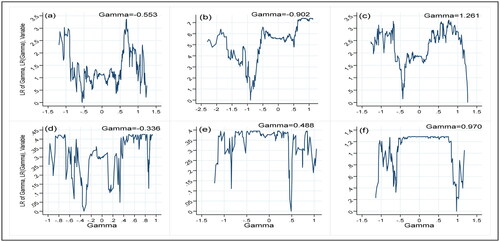
The threshold estimated is the point where the likelihood ratio function is equal to zero, which occurs at points −0.553, −0.902 and 1.261 in spring, summer and fall respectively for rainfall variability, and −0.336, 0.488 and 0.970 in spring, summer and fall respectively for temperature variability.

A closer look shows that before the threshold value, the variability in rainfall decreases in spring and summer, confirming the negative sign; while there is an increasing trend for variability in rainfall in fall. There is no clear trend for temperature variability except in summer, when there is a positive trend.

6. Conclusion and policy recommendation

In this paper, we introduced a GMM estimation to assess the impact of growing season variability in rainfall and temperature in Eastern Africa. We collected data from this part of Africa for the period 1961 to 2020. Contrary to Abraha-Kahsay and Hansen (2016), who incorporated disaggregated growing and non-growing seasons and assessed their impact, our main contribution was to go one step ahead and determine at which threshold levels such growing seasonal variability becomes harmful to agricultural output.

Our results reveal that growing season rainfall variability has an impact mainly in the major growing season. After introducing the GMM estimation, we find that the lag output was significant across all specifications. In the context of the rural economy that characterises Eastern Africa, the livelihoods of farmers depend on how they choose to allocate resources to generate the highest income possible, given the constraints they are facing. These decisions depend on the income that would be generated, making lag output one of the most important features in decision making. After controlling for endogeneity, the results reveal that growing-season rainfall variability affects output negatively, but there is no significant evidence that growing season temperature variability has an effect. However, we realise that the impact of growing season temperature and rainfall depends on the model specification used.

Using the dynamic panel threshold estimation, growing season rainfall threshold was −0.553 in spring with 95% confidence interval of [−1.222, 1,244]; −0.902 in summer, with 95% confidence interval of [−2.348, 0.59]; and 1.261 in fall with a 95% confidence interval of [−1.270, 1.261]. Any change in seasonal rainfall variability below the threshold will decrease agricultural output by 0.0127% in spring; in summer, if it goes beyond threshold then output will increase by 0.00832%. In the fall season, a change in rainfall variability below threshold means agricultural product will decrease by 0.0147%. In the case of growing season temperature, we found no significant effects.

From a policy standpoint, the relevance of growing season precipitation variability for agricultural output is particularly intriguing since its impacts are more easily offset by small-scale technology already utilised by local farmers. To mitigate the effect caused by the growing seasonal variability in precipitation, technologies such as flexible planting and rainwater harvesting. Also, irrigation and other practices to reduce the impact of growing season rainfall variability, such as implementing smart water-management systems that use drop-by-drop or sprinkler irrigation processes to improve agricultural output.

Cultivation practices like the Survival Strategies of Steppe Plants, to deal with seasonal variations can be considered as well. Warming might extend the growing season in frost-prone areas (temperate and arctic zones), allowing for longer-maturing seasonal cultivars with higher yields. Extending the planting season might result in more crops being grown each year. Because warming causes repeated highs in the warmer months above critical thresholds, a split season with a brief summer fallow might be feasible for short-period crops like wheat, barley, cereals, and a variety of other vegetable crops. In tropical and subtropical areas where the harvest season is controlled by precipitation or when cultivation begins later in the year, the ability to extend the planting season may be limited and depending on how precipitation patterns fluctuate. Therefore, new policies should be implemented by the government to encourage innovation in technology and raise agricultural output. In order to encourage agricultural investments, governmental tools like machinery purchase subsidies and agricultural insurance policies are crucial.

For many yields, the genetic component is considerable an alternative to a natural seed crop. The advantages of genetically modified crops are having a considerable impact on public perception and public policy decisions related to their usage.

However, it is important to highlight that relying solely on government action to achieve social quality and public policy is problematic. Furthermore, providing training for actors in the use of various methods for assisting farmers and groups of farmers, as well as in the entire subject of climate change, is vital at the local level. Adaptation is also a vital complement to mitigation strategies. Furthermore, while adaptation includes a wide range of characteristics and types, there are several adaptations that involve both the private agent and the government.

Clearly, there is still work to be done. Future research should hopefully look at the threshold below and over which variations in temperature and rainfall will affect a particular agricultural crop. As in this study, the agricultural production as a whole was taken into account. Crops may respond differently to climatic shocks.

Disclosure statement

No potential conflict of interest was reported by the author(s).

Notes

1 Ricardian approach estimates the impact of climate variables in the agriculture sector (Mendelsohn, 2014). Ricardian regression specification typically includes historical average precipitation, historical average temperature, and growing and non-growing seasons (Abraha-Kahsay & Hansen, 2016).

2 The quadratic term in Ricardian approach is used to define the net revenue climate response function in order to reflect its nonlinear structure, which shows how the marginal effect will vary as one goes away from the mean (Mendelsohn et al., 1994). The net revenue function has a U-shaped form when the quadratic component is positive (Huong et al., 2019), meaning increasing temperature during dry season significantly reduces the households’ net revenue.

3 Wang et al. (2009) revealed that at least one of the climate variables is significant in every season except for autumn temperature and summer precipitation. The fact that several of the squared coefficients of climate variables are significant suggests that the impacts of climate change on the crop net revenue are nonlinear. However, their findings revealed also that it is challenging to understand the coefficients themselves due to the quadratic structure of the climatic variables. Hence, determining a threshold is crucial.

4 Livestock capital input refers to FAO’s head count of cattle, sheep, and goats (Abraha-Kahsay & Hansen 2016; Barrios et al. 2008). In addition to include the most significant animal types, the proxy also overcomes the weighting problem raised by Barrios et al. (2008) by leaving out less significant animal groupings.

Appendix

Table A1. Test results.

Test	${\chi }^2$	F-statistic	p-Value
Modified Wald test for group
Heteroskedasticity	364.260		0.000
Serial correlation		1.785	0.266
Hausman	457.860		0.000

Table A2. Descriptive statistics of economic and climate data.

Variables	Mean	St. Dev
Dependent variable
Output (in millions of international US dollars)	7445.89	5911.00
Independent variables
Physical
Land (1000 persons)	31,227.30	34,764.56
Labour (1000 of hectares)	19,965.49	26,191.85
Machinery	3057.55	3835.89
Livestock (Head count of cattle, sheep, and goats in millions)	28.20	31.30
Irrigation (1000 of hectares)	0.49	0.53
Fertilizer (1000 of hectares)	21,549.26	36,587.19
Climate variables
Temperature	24.86	3.57
Precipitation	66.13	37.65
${\mathrm{\text{Variability}}}^{\mathrm{\text{Temp}}}$	0.06	0.35
${\mathrm{\text{Variability}}}^{\mathrm{\text{Precip}}}$	−0.54	7.37
countries	9
Sample	504

Table A3. Unit root test results.

Variables	LLC			Fisher
L$n(\mathit{\text{Output}})$	−4.440	(0.000)	1.822	(0.0342
L$n(\mathit{\text{Land}})$	−1.262	(0.001)	0.036	(0.005)
L$\mathrm{n}(\mathit{\text{Machinery}})$	−10.450	(0.000)	18.075	(0.000)
L$n(\mathit{\text{Livestock}})$	0.237	(0.006)	0.396	(0.000)
L$n(\mathit{\text{Labour}})$	−1.913	(0.028)	−0.684	(0.008)
L$\mathrm{n}(\mathit{\text{Irrigation}})$	−3.441	(0.000)	2.915	(0.002)
L$\mathrm{n}(\mathit{\text{Fertiliser}})$	−4.168	(0.000)	8.982	(0.000)
${\mathit{\text{Ln}}(\mathit{\text{Rainfall}}}_{\mathit{\text{Spring}}}$)	−11.262	(0.000)	40.345	(0.000)
${\mathit{\text{Ln}}(\mathit{\text{Rainfall}}}_{\mathit{\text{Summer}}}$)	−12.032	(0.000)	35.420	(0.000)
$\mathit{\text{Ln}}({\mathit{\text{Rainfall}}}_{\mathit{\text{fall}}}$)	−10.822	(0.000)	32.465	(0.000)
$\mathit{\text{Ln}}({\mathit{\text{Temp}}}_{\mathit{\text{Spring}}}$)	−7.384	(0.000)	17.320	(0.000)
$\mathit{\text{Ln}}({\mathit{\text{Temp}}}_{\mathit{\text{Summer}}}$)	−9.862	(0.000)	26.218	(0.000)
$\mathit{\text{Ln}}({\mathit{\text{Temp}}}_{\mathit{\text{fall}}}$)	−3.362	(0.000)	13.276	(0.000)
V ${\mathrm{\text{ariability}}}_{\text{spring}}^{\mathrm{\text{Rainfall}}}$	−10.809	(0.000)	35.779	(0.000)
V ${\mathrm{\text{ariability}}}_{\mathrm{\text{Summer}}}^{\mathrm{\text{Raonfall}}}$	−9.573	(0.000)	33.540	(0.000)
V ${\mathrm{\text{ariability}}}_{\mathrm{\text{Fall}}}^{\mathrm{\text{Rainfall}}}$	−11.971	(0.000)	34.258	(0.000)
V ${\mathrm{\text{ariability}}}_{\mathrm{\text{Spring}}}^{\mathrm{\text{Temp}}}$	−8.051	(0.000)	17.335	(0.000)
V ${\mathrm{\text{ariability}}}_{\mathrm{\text{Summer}}}^{\mathrm{\text{Temp}}}$	−10.316	(0.000)	24.097	(0.000)
V ${\mathrm{\text{ariability}}}_{\mathrm{\text{Fall}}}^{\mathrm{\text{Temp}}}$	−5.670	(0.000)	13.276	(0.000)

p-Value in parentheses.

Table A4. Fixed effects results of climate variability and agricultural output.

	(a) General	(b) Reduced	(c) Reduced	(d) Physical
VARIABLES	Ln(output)	Ln(output)	Ln(output)	Ln(output)
L$n(\mathit{\text{Land}})$	1.352***	1.338***	0.925 ***	0.333***
	(0.115)	(0.120)	(0.109)	(0.0781)
L$n(\mathit{\text{livestock}})$	0.423***	0.433***	0.624***	0.254***
	(0.108)	(0.107)	(0.126)	(0.0313)
L$n(\mathit{\text{labor}})$	0.0093	0.0032	0.539***	0.222***
	(0.063)	(0.0621)	(0.041)	(0.0265)
L$\mathrm{n}(\mathit{\text{machinery}})$	0.307	0.278	0.267	0.119
	(0.444)	(0.386)	(0.431)	(0.0143)
L$\mathrm{n}(\mathit{\text{irrigation}})$	0.370	0.370	0.249	0.127
	(0.412)	(0.397)	(0.447)	(0.0127)
L$\mathrm{n}(\mathit{\text{fertilizer}})$	0.237***	0.243***	0.341***	0.0725***
Mean Rain fall variables	(0.0277)	(0.0269)	(0.0302)	(0.0086)
${\mathit{\text{Ln}}(\mathit{\text{Rainfall}}}_{\mathit{\text{Spring}}}$)	0.421***	0.421***
	(0.0912)	(0.0907)
${\mathit{\text{Ln}}(\mathit{\text{Rainfall}}}_{\mathit{\text{Summer}}}$)	−0.0910
	(0.069)
$\mathit{\text{Ln}}({\mathit{\text{Rainfall}}}_{\mathit{\text{fall}}}$)	−0.333**	−0.382***
Mean Temperature Variables	(0.114)	(0.109)
$\mathit{\text{Ln}}({\mathit{\text{Temp}}}_{\mathit{\text{Spring}}}$)	2.716*	2.156
	(1.377)	(1.322)
$\mathit{\text{Ln}}({\mathit{\text{Temp}}}_{\mathit{\text{Summer}}}$)	−4.314***	−4.631***
	(1.174)	(1.121)
$\mathit{\text{Ln}}({\mathit{\text{Temp}}}_{\mathit{\text{fall}}}$)	−4.346***	−3.369***
Within growing season rainfall variables	(1.082)	(0.810)
V ${\mathrm{\text{ariability}}}_{\text{spring}}^{\mathrm{\text{Rainfall}}}$	−0.120***	−0.114***	−0.0805*
	(0.0367)	(0.0363)	(0.0439)
V ${\mathrm{\text{ariability}}}_{\mathrm{\text{Summer}}}^{\mathrm{\text{Raonfall}}}$	−0.196***	−0.187***	−0.119***
	(0.0284)	(0.0278)	(0.0307)
V ${\mathrm{\text{ariability}}}_{\mathrm{\text{Fall}}}^{\mathrm{\text{Rainfall}}}$	0.019		0.00705
Within growing season temperature variables	(0.0366)		(0.00443)
V ${\mathrm{\text{ariability}}}_{\mathrm{\text{Spring}}}^{\mathrm{\text{Temp}}}$	0.109**	0.125***	0.189***
	(0.0433)	(0.041)	(0.0522)
V ${\mathrm{\text{ariability}}}_{\mathrm{\text{Summer}}}^{\mathrm{\text{Temp}}}$	−0.0656		−0.089
	(0.0414)		(0.0506)
V ${\mathrm{\text{ariability}}}_{\mathrm{\text{Fall}}}^{\mathrm{\text{Temp}}}$	−0.0125		0.072
	(0.0414)		(0.0502)
Year	0.0317***	0.0321***	0.0321***	0.0107***
	(0.00245)	(0.00237)	(0.00237)	(0.00111)
Constant	−40.401***	−41.723***	−41.723***	−24.67***
	(5.293)	(5.628)	(5.130)	(1.529)
Observations	540	540	540	540
Number of id	9	9	9	9

Standard errors in parentheses *** denotes significance at 1%, ** denotes significance at 5%, * denotes significance at 10% level respectively.

References

- Abbas, S., & Mayo, Z. A. (2021). Impact of temperature and rainfall on rice production in Punjab, Pakistan. Environment, Development and Sustainability, 23(2), 1706–1728. https://doi.org/10.1007/s10668-020-00647-8
- Abdi, A. H., Warsame, A. A., & Sheik‑Ali, I. A. (2022). Modelling the impacts of climate change on cereal crop production in East Africa: Evidence from heterogeneous panel cointegration analysis. Environmental Science and Pollution Research, 30(12), 35246–35257. https://doi.org/10.1007/s11356-022-24773-0
- Abraha-Kahsay, G., & Hansen, L. G. (2016). The effect of climate change and adaptation policy on agriculture production in Eastern Africa. Ecological Economics, 121, 54–64. https://doi.org/10.1016/j.ecolecon.2015.11.016
- Amare, M., Jensen, N. D., Shiferaw, B., & Cissé, J. D. (2018). Rainfall shocks and agricultural productivity: Implication for rural household consumption. Agricultural Systems, 166, 79–89. https://doi.org/10.1016/j.agsy.2018.07.014
- Anderson, R., Bayer, P. E., & Edwards, D. (2020). Climate change and the need for agricultural adaptation. Current Opinion in Plant Biology, 56, 197–202. https://doi.org/10.1016/j.pbi.2019.12.006
- Antle, J. M. (1983). Testing the stochastic structure of production: A flexible moment based approach. Journal of Business & Economic Statistics, 1(3), 192–201. https://doi.org/10.2307/1391337
- Arellano, M., & Bover, O. (1995). Another look at the instrumental variable estimation of error- components models. Journal of Econometrics, 68(1), 29–51. https://doi.org/10.1016/0304-4076(94)01642-D
- Bahaga, T. K., Mengistu, T. G., Kucharski, F., & Diro, G. T. (2014). Potential predictability of the sea-surface temperature forced equatorial East African short rains interannual variability in the 20th century. Quarterly Journal of the Royal Meteorological Society, 141(686), 16–26. https://doi.org/10.1002/qj.2338
- Barrios, S., Ouattara, B., & Strobl, E. (2008). The impact of climatic change on agricultural production: Is it different for Africa? Food Policy. 33(4), 287–298. https://doi.org/10.1016/j.foodpol.2008.01.003
- Bedeke, S. B. (2023). Climate change vulnerability and adaptation of crop producers in sub-Saharan Africa: A review on concepts, approaches and methods. Environment, Development and Sustainability, 25(2), 1017–1051. https://doi.org/10.1007/s10668-022-02118-8
- Blanc, E. (2012). The impact of climate change on crop yields in sub-Saharan Africa. American Journal of Climate Change, 01(01), 1–13. https://doi.org/10.4236/ajcc.2012.11001
- Blundell, R., & Bond, S. (1998). Initial conditions and moment restrictions in dynamic panel data models. Journal of Econometrics, 87(1), 115–143. https://doi.org/10.1016/S0304-4076(98)00009-8
- Cabas, J., Weersink, A., & Olale, E. (2009). Crop yield response to economic, site and climatic variable. Climatic Change, 101(3–4), 599–616. https://doi.org/10.1007/s10584-009-9754-4
- Caner, M., & Hansen, B. E. (2004). Instrumental variable estimation of a threshold model. Econometric Theory, 20(05), 813–843. https://doi.org/10.1017/S0266466604205011
- Chandio, A. A., Jiang, Y., Rehman, A., & Rau, A. (2020). Short and long-run impacts of climate change on agriculture: An empirical evidence from China. International Journal of Climate Change Strategies and Management, 12(2), 201–221. https://doi.org/10.1108/IJCCSM-05-2019-0026
- Chandio, A. A., Jiang, Y., Fatima, T., Ahmad, F., Ahmad, M., & Li, J. (2022). Assessing the impacts of climate change on cereal production in Bangladesh: Evidence from ARDL modeling approach. International Journal of Climate Change Strategies and Management, 14(2), 125–147. https://doi.org/10.1108/IJCCSM-10-2020-0111
- Chen, S., & Gong, B. (2021). Response and adaptation of agriculture to climate change: Evidence from China. Journal of Development Economics, 148, 102557. https://doi.org/10.1016/j.jdeveco.2020.102557
- Choi, I. (2001). Unit root tests for panel data. Journal of International Money and Finance, 20(2), 249–272. https://doi.org/10.1016/S0261-5606(00)00048-6
- Conway, D., Allison, E., Felstead, R., & Goulden, M. (2005). Rainfall variability in East Africa: Implications for natural resources management and livelihoods. Philosophical Transactions. Series A, Mathematical, Physical, and Engineering Sciences, 363(1826), 49–54. https://doi.org/10.1098/rsta.2004.1475
- Conway, D., & Schipper, E. L. (2011). Adaptation to climate change in Africa: Challenges and opportunities identified from Ethiopia. Global Environmental Change, 21(1), 227–237. https://doi.org/10.1016/j.gloenvcha.2010.07.013
- Constable, A. J., Melbourne-Thomas, J., Corney, S. P., Arrigo, K. R., Barbraud, C., Barnes, D. K. A., Bindoff, N. L., Boyd, P. W., Brandt, A., Costa, D. P., Davidson, A. T., Ducklow, H. W., Emmerson, L., Fukuchi, M., Gutt, J., Hindell, M. A., Hofmann, E. E., Hosie, G. W., Iida, T., … Ziegler, P. (2014). Climate change and Southern Ocean ecosystems I: Howchanges in physical habitats directly affect marine biota. Global Change Biology, 20(10), 3004–3025.https://doi.org/10.1111/gcb.12623
- Espoir, D. K., Mudiangombe, B. M., Bannor, F., Sunge, R., & Mubenga-Tshitaka, J. L. (2022). CO2 emissions and economic growth: Assessing the heterogeneous effects across climate regimes in Africa. The Science of the Total Environment, 804, 150089. https://doi.org/10.1016/j.scitotenv.2021.150089
- FAO. (2008). Agriculture mechanization in Africa time for action: planning investment for enhanced agricultural productivity. In Report of an Expert Group Meeting January 2008. FAO. http://www.fao.org/3/k2584e/k2584e.pdf
- FAO. (2015). The economic lives of smallholder farmers: Analysis based on household data from nine countries. FAO. http://www.fao.org/3/a-i5251e.pdf
- FAOSTAT. (2011). FAO statistical database. https://www.fao.org/faostat/en/#data/QV
- Gebrechorkos, S. H., Hülsmann, S., & Bernhofer, C. (2020). Analysis of climate variability and droughts in East Africa using high-resolution climate data products. Global and Planetary Change, 186, 103130. https://doi.org/10.1016/j.gloplacha.2020.103130
- Gebrechorkos, S. H., Hülsmann, S., & Bernhofer, C. (2019). Long-term trends in rainfall and temperature using high- resolution climate datasets in East Africa. Scientific Reports, 9(1), 11376. https://doi.org/10.1038/s41598-019-47933-8
- Gomez-Zavaglia, A., Mejuto, J. C., & Simal-Gandara, J. (2020). Mitigations of emerging implications of climate change on food production systems. Food Research International (Ottawa, Ont.), 134, 109256. https://doi.org/10.1016/j.foodres.2020.109256
- Gommes, R., & Petrassi, F. (1996). Rainfall variability and drought in sub-Saharan Africa, Environment and Natural Resources Service, FAO Research, Extension and Training Division. http://www.fao.org/3/au042e/au042e.pdf.
- Hayami, Y., & Ruttan, V. W. (1970). Agriculture productivity differences among countries. American Economic Review, 60(5), 895–911. https://www.jstor.org/stable/1818289
- Huong, N. T., Bo, Y. S., & Fahad, S. (2019). Economic impact of climate change on agriculture using Ricardian approach: A case of northwest Vietnam. Journal of the Saudi Society of Agricultural Sciences, 18(4), 449–457. https://doi.org/10.1016/j.jssas.2018.02.006
- Hansen, B. E. (1999). Threshold effects in non-dynamic panels: Estimation, testing, and inference. Journal of Econometrics, 93(2), 345–368. https://doi.org/10.1016/S0304-4076(99)00025-1
- Intergovernmental Panel on Climate Change (IPCC). (2007). Contribution of working group I to the fourth assessment report. Cambridge University Press.
- Kansiime, M. K., Van Asten, P., & Sneyers, K. (2018). Farm diversity and resource use efficiency: Targeting agriculture policy interventions in East Africa farming systems. NJAS: Wageningen Journal of Life Sciences, 85(1), 32–41. https://doi.org/10.1016/j.njas.2017.12.001
- Karimi, V., Karami, E., & Keshavarz, M. (2018). Climate change and agriculture: Impacts and adaptive responses in Iran. Journal of Integrative Agriculture, 17(1), 1–15. https://doi.org/10.1016/S2095-3119(17)61794-5
- Kremer, S., Bick, A., & Nautz, D. (2013). Inflation and growth: New evidence from a dynamic panel threshold analysis. Empirical Economics, 44(2), 861–878. https://www.econstor.eu/bitstream/10419/39331/1/60792313X.pdf https://doi.org/10.1007/s00181-012-0553-9
- Lachaud, M. A., Bravo-Ureta, B. E., & Ludena, C. E. (2022). Economic effects of climate change on agricultural production and productivity in Latin America and the Caribbean (LAC). Agricultural Economics, 53(2), 321–332. https://doi.org/10.1111/agec.12682
- Lal, M. (2011). Implications of climate change in sustained agricultural productivity in South Asia. Regional Environmental Change, 11(S1), 79–94. https://doi.org/10.1007/s10113-010-0166-9
- Levin, A., Chien-Fu, C., & Chia-Shang, J. C. (2002). Unit root tests in panel data: Asymptotic and finite-sample properties. Journal of Econometrics, 108(1), 1–24. https://doi.org/10.1016/S0304-4076(01)00098-7
- Lippert, C., Krimly, T., & Aurbacher, J. (2009). A Ricardian analysis of the impact of climate change on agriculture in Germany. Climatic Change, 97(3–4), 593–610. https://doi.org/10.1007/s10584-009-9652-9
- Lobell, D. B., & Burke, M. B. (2010). On the use of statistical models to predict crop yield responses to climate change. Agricultural and Forest Meteorology, 150(11), 1443–1452. https://doi.org/10.1016/j.agrformet.2010.07.008
- Lobell, D. B., Bänziger, M., Magorokosho, C., & Vivek, B. (2011). Nonlinear heat effects on African maize as evidenced by historical yield trials. Nature Climate Change, 1(1), 42–45. https://doi.org/10.1038/nclimate1043
- Lowder, S. K., Sánchez, M. V., & Bertini, R. (2019). Farms, family farms, farmland distribution and farm labour: What do we know today? In FAO agricultural development economics economics working paper 19-08. FAO.
- McCarl, B. A., Villavicencio, X., & Wu, X. (2008). Climate change and future analysis: is stationary dying? American Journal of Agricultural Economics, 90(5), 1241–1247. https://www.jstor.org/stable/20492379 https://doi.org/10.1111/j.1467-8276.2008.01211.x
- Mendelsohn, R., Nordhaus, W. D., & Shaw, D. (1994). The impact of global warming on agriculture: A Ricardian analysis. The American Economic Review, 84(4), 753–771. https://www.jstor.org/stable/2118029
- Mendelsohn, R. (2009). The impact of climate change on agriculture in developing countries. Journal of Natural Resources Policy Research, 1(1), 5–19. https://doi.org/10.1080/19390450802495882
- Mendelsohn, R. (2014). The impact of climate change on agriculture in Asia. Journal of Integrative Agriculture, 13(4), 660–665. https://doi.org/10.1016/S2095-3119(13)60701-7
- Mishra, D., & Sahu, N. C. (2014). Economic impact of climate change on agriculture sector of Coastal Odisha. APCBEE Procedia, 10, 241–245. https://doi.org/10.1016/j.apcbee.2014.10.046
- Molua, E. L., & Lambi, C. M. (2007). The economic impact of climate change on agriculture in Cameroon. The World Bank Policy Research Working, 4364. Development Research Group Sustainable Rural and Urban Development Team, The World Bank. https://papers.ssrn.com/sol3/papers.cfm?abstract_id=1016260.
- Mubenga-Tshitaka, J. L., Dikgang, J., Muteba Mwamba, J. W., & Gelo, D. (2023). Climate variability impacts on agricultural output in East Africa. Cogent Economics & Finance, 11(1), 2181281. https://doi.org/10.1080/23322039.2023.2181281
- Ngoma, H., Finn, A., & Kabisa, M. (2023). Climate shocks, vulnerability, resilience and livelihoods in rural Zambia. Climate and Development, 16(6), 490–501. https://doi.org/10.1080/17565529.2023.2246031
- Nguyen, C. T., & Scrimgeour, F. (2022). Measuring the impact of climate change on agriculture in Vietnam: A panel Ricardian analysis. Agricultural Economics, 53(1), 37–51. https://doi.org/10.1111/agec.12677
- Niang, A., Amrani, F., Salhi, M., Grelu, P., & Sanchez, F. (2014). Rains of solitons in a figure of eight passive mode-locked fiber laser. Applied Physics B, 116(3), 771–775. https://doi.org/10.1007/s00340-014-5760-y
- Nickell, S. (1981). Biases in dynamic models with fixed effects. Econometrica, 49(6), 1417–1426. https://doi.org/10.2307/1911408
- Noy, I. (2009). The macroeconomic consequences of disasters. Journal of Development Economics, 88(2), 221–231. https://doi.org/10.1016/j.jdeveco.2008.02.005
- Owusu, K., & Waylen, P. R. (2013). Identification of historic shifts in daily rainfall regime, Wenchi, Ghana. Climatic Change, 117(1–2), 133–147. https://doi.org/10.1007/s10584-013-0692-9
- Pickson, R. B., He, G., & Boateng, E. (2022). Impacts of climate change on rice production: Evidence from 30 Chinese provinces. Environment, Development and Sustainability, 24(3), 3907–3925. https://doi.org/10.1007/s10668-021-01594-8
- Poudel, S., & Kotani, K. (2013). Climatic impacts on crop yield and its variability in Nepal: Do they vary across seasons and altitude? Climatic Change, 116(2), 327–355. https://doi.org/10.1007/s10584-012-0491-8
- Regan, P. M., Kim, H., & Maiden, E. (2019). Climate change, adaptation, agricultural output. Regional Environmental Change, 19(1), 113–123. https://doi.org/10.1007/s10113-018-1364-0
- Roodman, D. (2009). How to do xtabond2: An introduction to difference and system GMM in Stata. The Stata Journal: Promoting Communications on Statistics and Stata, 9(1), 86–136. https://doi.org/10.1177/1536867X0900900106
- Rosenzweig, C., Casassa, G., Karoly, D. J., Imeson, A., Liu, C., Menzel, A., Rawlins, S., Root, T. L., Seguin, B., & Tryjanowski, P. (2007). Assessment of observed changes and responses in natural and managed systems. In M. L. Parry, O. F. Canziani, J. P. Palutikof, P. J. van der Linden, & C. E. Hanson (Eds.), Climate Change 2007: Impacts, Adaptation and Vulnerability. Contribution of Working Group II to the Fourth Assessment Report of the Intergovernmental Panel on Climate Change (pp. 79–131). Cambridge University Press.
- Rowhani, P., Lobell, D. B., Linderman, M., & Ramankutty, N. (2011). Climate variability and crop production in Tanzania. Agricultural and Forest Meteorology, 151(4), 449–460. https://doi.org/10.1016/j.agrformet.2010.12.002
- Rui-Li, L., & Geng, S. (2013). Impact of climate change on agriculture and adaptive strategies in China. Journal of Integrative Agriculture, 12(8), 1402–1408. https://doi.org/10.1016/S2095-3119(13)60552-3
- Runge, C. F., Senauer, B., Pardey, P. G., & Rosegrant, N. W. (2004). Ending hunger in Africa: prospects for the small farmer. International Food Policy Research Institute (IFRI).
- Schlenker, W., & Roberts, M. J. (2009). Nonlinear temperature effects indicate severe damages to U.S. crop yields under climate change. Proceedings of the National Academy of Sciences of the United States of America, 106(37), 15594–15598. https://doi.org/10.1073/pnas.0906865106
- Schreck, C. Z., & Semazzi, F. H. (2004). Variability of the climate of Eastern Africa. International Journal of Climatology, 24(6), 681–701. https://doi.org/10.1002/joc.1019
- Schlenker, W., & Lobell, D. B. (2010). Robust negative impacts of climate change on African agriculture. Environmental Research Letters, 5(1), 014010. https://doi.org/10.1088/1748-9326/5/1/014010
- Shahzad, A., Ullah, S., Dar, A. A., Sardar, M. F., Mehmood, T., Tufail, M. A., Shakoor, A., & Haris, M. (2021). Nexus on climate change: Agriculture and possible solution to cope future climate change stresses. Environmental Science and Pollution Research International, 28(12), 14211–14232. https://doi.org/10.1007/s11356-021-12649-8
- Toret, A., Bassu, S., Asseng, S., Zampieri, M., Ceglar, A., & Royo, C. (2022). Climate service driven adaptation may alleviate the impact of climate change in agriculture. Communications Biology, 5(1), 1235. https://doi.org/10.1038/s42003-022-04189-9
- Van den Broeck, G., & Kilic, T. (2018). Dynamic of off-farm employment in sub-Saharan Africa: a gender perspective. eLibrary, World Bank. https://elibrary.worldbank.org/doi/pdf/10.1596/1813-9450-8540
- Victor, U. S., Srivasta, N. N., Subba-Rao, A. V. M., & Ramana-Roa, B. V. (1996). Managing the impact of seasonal rainfall variability through response farming at a semi-arid tropical location. Current Science, 71(5), 392–397. https://doi.org/10.1016/j.atmosres.2019.03.023
- Wang, J., Mendelsohn, R., Dinar, A., Huang, J., Rozelle, S., & Zhang, L. (2009). The impact of climate change on China’s agriculture. Agricultural Economics, 40(3), 323–337. https://doi.org/10.1111/j.1574-0862.2009.00379.x
- Ward, P. S., Florax, R. J., & Flores-Lagunes, A. (2014). Climate change and agriculture productivity in sub-Saharan Africa, a spacial sample selection model. European Review of Agricultural Economics, 41(2), 199–226. https://doi.org/10.1093/erae/jbt025
- Warsame, A. A., Sheik-Ali, I. A., Ali, A. O., & Sarkodie, S. A. (2021). Climate change and crop production nexus in Somalia: An empirical evidence from ARDL technique. Environmental Science and Pollution Research International, 28(16), 19838–19850. https://doi.org/10.1007/s11356-020-11739-3
- Wichern, J., Van Wijk, M. T., Descheemaeker, K., Frelat, R., Van Asten, P. J. A., & Giller, K. E. (2017). Food availability and livelihood strategies among rural households across Uganda. Food Security, 9(6), 1385–1403. https://doi.org/10.1007/s12571-017-0732-9
- World Bank. (2007). World Development Report, 2008: Agriculture for Development. Oxford University Press.
- Wooldridge, J. M. (2002). Econometric analysis of cross section and panel data. MIT Press.
- You, L., Rosegrant, M. W., Wood, S., & Sun, D. (2009). Impact of growing season temperature on wheat production in China. Agricultural and Forest Meteorology, 149(6–7), 1009–1014. https://doi.org/10.1016/j.agrformet.2008.12.004