A comparative VaR analysis between low-frequency and high-frequency conditional EVT models during COVID-19 crisis

Abstract

The aim of this paper is to assess whether the availability of high-frequency data enhances the accuracy of extreme market risk estimation in comparison to low-frequency data by using Value-at-risk (VaR) and Expected shortfall (ES). The sample data used for analysis comprised the daily closing stock prices and 5-minute intraday stock prices of DJIA, FTSE100, BOVESPA, and MERVAL Index from 2014 to 2022. The data analysis was done to compare the performance of two-stages hybrid methods called conditional EVT that combined the GARCH, RV and HAR specification models with the EVT approach. To assess the accuracy of the VaR forecasts, out-of-sample VaR forecast was backtested by using unconditional coverage (UC) and conditional coverage (CC) tests. The VaR backtesting procedure also incorporated the utilization loss function which are the regulatory loss function (RLF) and the firm’s loss function (FLF). The accuracy of the forecasted ES was backtested by using the generalized breach indicator (GBI) method. The findings of this research emphasized that high-frequency conditional EVT, incorporating the HAR specification outperformed the low-frequency conditional EVT in predicting market risk during periods characterized by extreme returns. Based on the VaR and ES measure, the HAR-EVT typed models are the best performance model compared to the GARCH-EVT and RV-EVT typed models during both crisis and non-crisis periods. This research study contributes to the current literature on the forecasting ability of risk models by concentrating on the hybrid model of long-memory models (FIEGARCH, RV-FIEGARCH and HAR-FIEGARCH) for with the EVT approach.

Impact statement

The analysis compares the performance of two-stages hybrid methods called conditional EVT that combined the GARCH, RV and HAR specification models with the EVT approach during non-crisis and crisis COVID-19 pandemic. Based on the VaR and ES measure, the HAR-EVT typed models are the best performance model compared to the GARCH-EVT and RV-EVT typed models. The findings of this research study are also beneficial to market participants, especially those who engage in high-frequency trading to utilize the RV and HAR models as well the application of the EVT model to measure the potential risks and detect any vulnerabilities in financial systems especially during a sudden market crash.

Keywords:

• Conditional EVT
• expected shortfall
• high-frequency data
• value-at-risk

REVIEWING EDITOR:

• Xibin Zhang, Econometrics and Business Statistics, Monash University, Australia

SUBJECTS:

• Economics
• Finance
• Business, Management and Accounting

1. Introduction

The degree of stock market volatility should raise significant concerns among different stakeholders, including investors, regulators, and financial institutions, to prevent potential economic challenges in the future. Historical records indicate that fluctuations in stock prices during periods of market turbulence can exert a considerable influence on financial downturns, as evidenced by events like the catastrophic Black Monday in October 1987 and Black Friday in October 1989. These unexpected and rare historical occurrences instilled concerns about economic recession and had repercussions on numerous countries across the globe. Another notable extreme event that caused a devastating financial crisis was the Asian financial crisis of 1997. This crisis has impacted financial markets in terms of extreme price movements which lead to the depreciation in currency and a crash in the stock market globally. This crisis had heightened volatility not only in Asian counties as well as other nations which hesitate foreign investors to invest in the Asian market. Due to that, most of the banks and financial institutions are collapsed which gives severe losses for creditors and investors. Further to that, the global financial crises 2007–2008 crisis stands as the most terrifying crisis. This crisis derived from a subprime mortgage lending crisis in 2007 and quickly accelerated into a worldwide banking crisis with the collapse of Lehman Brothers investment bank in September 2008. Regardless of substantial efforts to sustain the fallout, the damage proved uncontrollable, plunging the global economy into a deep recession. On December 31, 2019, the emergence of the coronavirus (COVID-19) began in China and subsequently spread to 220 countries and territories worldwide. On March 11, 2020, the World Health Organization (WHO) officially declared it a global pandemic (Kickbusch et al., 2020). The emergence of COVID-19 cases had a profound impact on the financial market. The rapid spread of the virus and the subsequent global lockdown measures implemented to contain it led to significant disruptions in economic activities and investor sentiment. The uncertainty surrounding the duration and severity of the pandemic caused widespread volatility and instability in financial markets as reported by Ullah (2022). The global stock markets experienced sharp declines as investors reacted to the escalating health crisis and its potential economic implications. The concerns regarding a worldwide economic downturn, diminished consumer expenditure, and disrupted supply chains led to significant selloffs and declines in the financial markets. There are recent studies by (Basuony et al., 2022; Hui & Chan, 2022; Rakshit & Neog, 2022) that found the impact of COVID-19 in global stock price by exhibited large volatility and risk uncertainty. The impact of financial crises on the stock markets as discussed above gives motivation to this study to include the recent COVID-19 period as the sample data for analysis. This choice is due to the absence of prior research regarding the efficiency of the high-frequency conditional EVT in forecasting the stock market risk during the COVID-19 period.

The analysis of this study includes the application of the heterogeneous market hypothesis (HMH) introduced by Dacorogna et al. (2001). According to HMH, investors follow the nonlinear trading behaviours of heterogeneous market participants where it is impossible for one price to reflect everyone’s information even when each investor receives similar information as claimed by the efficient market hypothesis (EMH) introduced by Fama (1965). Due to the heterogeneity perspective, there are various trading strategies which produce uncertainty of risk or volatility cascade and created the long memory property in the financial markets as mentioned by Cheong et al. (2016). Based on the HMH framework, the stock market returns were analyzed by considering how the market participants react to past information or news at different time horizons (daily, weekly and monthly). This paper considers the recent model introduced by researchers that incorporates the HMH framework called the heterogeneous autoregressive (HAR) model. The HAR model is an extension of the autoregressive conditional heteroskedasticity (ARCH) model that considers the long memory property observed in financial time series. The HAR model also aligns with the HMH theory because it considers the varying responses of different investor groups by incorporating lagged volatility measures at different time scales (short-term, medium-term, and long-term).

Based on previous research done in the risk forecasting field, the efficacy of risk estimation models selected are impacted by various elements, such as the type of risk model used, the type of data used (daily or intraday data) and the specific economics conditions under examination. Therefore, these two elements will be included in this study to see the efficiency of the low-frequency and high-frequency models in forecasting the stock market risk. With the rise of high-frequency data, the stock market now offers more information to investors. In today’s context, data can be gathered within seconds, such as 1-second intraday stock prices, contrasting with the past when data was collected at the close of the trading day. As the data undergoes frequent updates, it provides more recent and accurate information on market movements, thereby offering an advanced depiction of the current market conditions. During a financial crisis period, the quickest and most updated information is important so that investors can respond to any market volatility and uncertainty in the fastest way. The advantages of this new high-frequency data give motivation to this study to apply the high-frequency data (intraday data) to see whether it outperformed the low-frequency data (daily data) in forecasting the stock market risk especially during the financial crisis.

Previous literature has established the effectiveness of using the GARCH model in forecasting stock market risk based on low-frequency data (daily returns) in financial time series analysis. The GARCH model, with its ability to capture volatility clustering and persistence, has been widely employed and found to be suitable for modeling and forecasting volatility in various financial markets. At present, the accessibility of high-frequency data has spurred researchers to delve into alternative risk forecasting models, moving beyond the conventional GARCH model. Given that researchers have had sustained attention with the existence of long memory in daily returns, it is also imperative to examine the presence of long memory in intraday returns, especially regarding the RV and HAR specifications which give another motivation of this study. It is known that during periods of market turbulence, the financial stock market is vulnerable to extreme fluctuations, making the measurement of market risk a paramount concern for risk-averse investors. In this research, the utilization of high-frequency models based on the RV and HAR specifications are applied with the EVT approach. By employing the hybrid approach of high-frequency models with EVT, it assumed to improve the estimation of tail risk by more accurately capturing extreme market events. While the HAR model focuses on the volatility cascade across different investment horizons, the statistical framework of EVT facilitates the modeling and analysis by focusing on the extreme returns of tail distributions.

The hybrid method that combining any low-frequency or high frequency models with the EVT approach is generally called the conditional EVT model. Previous research on the conditional EVT model has been proven to enhance the ability to forecast and assess risk during turbulent market conditions, however mostly the research used daily returns as the volatility proxy. Due to the emergence of high-frequency data, researchers have started to explore how the intraday returns based on the RV specification help to improve the risk forecast. Further to the introduction of the HMH theory researchers try to combine the HAR model with the EVT approach. The finding by Louzis et al. (2007) found that the combined HAR-GARCH-EVT model, which incorporates the conditional heteroscedasticity of the HAR errors, demonstrates superior performance overall and produces precise estimates of VaR that effectively minimize Basel II regulatory capital requirements. The model’s accuracy is evident in both the full out-of-sample period and the specific crisis period of 2007–2009. Further research has been done on the accuracy of the HAR-EVT models in forecasting the stock market risk. The availability of high-frequency data gives another area of research on the efficiency of the low-frequency conditional EVT models compared to the high-frequency conditional EVT models. Researchers found that mostly, by comparing the high-frequency data, the conditional EVT performed better. The adoption of realized volatility as the volatility estimator of high-frequency data shows better prediction than the daily returns. Numerous studies have been conducted to substantiate the benefits of incorporating the RV specification as a hybrid model alongside the EVT approach. The current research also employs the RV specification derived from the HAR model in the context of the conditional EVT model; however, this area of study remains relatively unexplored. This study aims to contribute to the current literature on the forecasting ability of risk models by concentrating on the long-memory models of FIEGARCH, RV-FIEGARCH and HAR-FIEGARCH models with the EVT approach which has not been explored yet. The findings of the study will contribute to the grasp of how different type of data frequencies can influence stock market risk forecasting and provide accurate models to be used in any risk management practices and investment strategies.

Despite the advantage of high-frequency data researchers argue on whether it’s worth it to use high-frequency data due to its higher cost such as a study done by Lyócsa et al. (2021). Instead of the higher cost, it also requires more time to analyze compared to the low-frequency data. For investors and traders with large capital, the advantages of using this high-frequency data may outweigh the costs. The ability of this high-frequency data to quickly respond to market fluctuations will benefit them in increasing the capital invested and minimizing the potential loss. However, for other small investors and traders, the expenses associated with acquiring and analyzing high-frequency data will be the main barrier. In such instances, the low-frequency data, which is generally more affordable and accessible will be chosen. Some researchers which rely on low-frequency data will miss opportunities offered by high-frequency data especially in the current big data era where the growth of big data application database solutions and analytics is anticipated to expand by $12 billion in 2027 (Djuraskovic, 2023). The decision to utilize high-frequency data should be based on a detail evaluation of the potential advantages and disadvantages, as well as an understanding of how the data will be employed and what specific trading strategies or investment objectives it will support. The cost issue gives additional motivation of this study to explore whether the potential benefits of employing high-frequency data in data-rich markets outweigh or hold value when contrasted with low-frequency data. The question that lingers is whether this cost will ultimately yield substantial value in the context of modeling and forecasting financial markets.

2. Literature review

Volatility forecasting through the application of EVT has gained considerable attention among researchers. EVT provides a framework for analyzing extreme events and tail behavior in financial markets. By focusing on extreme observations, EVT enables the estimation of tail probabilities and extreme quantiles, which are crucial for volatility forecasting. EVT stands out as the optimal choice for analyzing the tail distribution characterized by extreme events. Extensive studies have been done to study the accuracy of the EVT approach compares other alternatives models in forecasting the stock market risk. A study done by Mcneil and Frey (2000) found that the hybrid model GARCH-EVT is effective to deals with asymmetric tail distributions on the S&P Index. A further research study by Paul and Sharma (2018) found that EVT is reliable in estimating the VaR and ES compared to other models that are not combined with EVT. A study done by Soltane et al. (2012) supports that the combination of the GARCH model and EVT outperforms the conventional standalone EVT model in predicting stock market volatility during extreme events. Another research conducted by Altun and Tatlidil (2015) which analyzed the ISE-100, S&P-500, and Nikkei-225 indexes, found that the GARCH-EVT model outperforms compared to standalone GARCH model. Additionally, research done by Youssef et al. (2015) found that the FIAPARCH-EVT model performs better in predicting one-day-ahead VaR compared to FIGARCH-EVT and HYGARCH-EVT. Another research done by Tabasi et al. (2019) shown the superiority of the GARCH-EVT model over the simple skewed-t GARCH model in estimating stock market risk during the capital depression period of the Tehran Stock Exchange. A study done by Omari et al. (2020) found that the GARCH-EVT model significantly improved VaR forecasting on the daily returns data of twelve major international stock indices. Further research done by Roy (2022) found that the GARCH-EVT models outperformed other models in forecasting intraday VaR during the COVID-19 pandemic. Additionally, study done by Jin et al. (2022) found that the GARCH-EVT-copula approach is the best to measure the VaR and ES before and during the COVID-19 pandemic. Recent study by Zhao et al. (2023) found that the GARCH-EVT-Copula-CoVaR model is accurate in forecasting the spillover risk impact of global oil prices on Chinese sectoral stock markets.

The new revolution of high-frequency data has encouraged researchers to use high frequency data that is based on intraday data to forecast the stock market risk. The realized volatility becomes new latent volatility used to estimate the VaR and ES instead of the daily returns’ volatility. New recent research used the combination realized volatility models and the EVT approach and the result shown that it has more advantages and reliable estimates compared to low-frequency models that used daily returns series. A study done by Watanabe (2012) examines the efficacy of the realized GARCH model in the US equity market. Subsequently, (Paul & Sharma, 2018) extend the analysis of Watanabe (2012) and conclude that the realized-GARCH EVT models demonstrate superior forecasting performance in estimating VaR and ES Another research done by Zhang and Zhang (2016) showed that the EGARCH model combined with the EVT approach does very well in predicting a critical loss for precious metal markets. According to Tabasi et al. (2019) the GARCH-EVT model enables a correct VaR estimation also in this market and outperforms the simple GARCH model with Student’s t and normal distributions for residuals. As discussed earlier, the HAR model, which captures the heterogeneity of market participants’ trading behaviors, has shown promise in capturing volatility dynamics at different time scales. The finding by Huang et al. (2016) demonstrates that the HAR-GARCH specification more effectively captures the persistent memory patterns in volatility when contrasted with the conventional GARCH model. Another research done by Tao et al. (2018) discovered that the HAR-RV models surpasses its conventional counterparts in VaR performance. The finding by Zahid et al. (2022) shows that the HAR-GARCH model exhibited superior forecasting precision for Bitcoin volatility when contrasted with alternative realized volatility models. Recent study by Maaz et al. (2023) show that the GARCH-EVT is superior in predicting the risk of high-frequency returns data at 15-minute intervals in the metal market.

As discussed in the Introduction section, the HAR model can capture the heterogeneity of market participants’ trading behaviors and creates a volatility cascade throughout the short to long-term investment period. By combining the HAR model with EVT, it assumes to add prediction of rare and extreme market events at different levels of market volatilities including short-term, medium-term, and long-term. Previously research by Louzis et al. (2007) found that the asymmetric HAR-EVT model is the best model to forecast the VaR. Another finding by Sojka (2015) shows that HAR-RV, HAR-RV-J and ARFIMA are accurate to forecast the daily and intraday returns with comparable results where the daily returns scored the minimum value of RLF while the intraday returns scored the minimum value of FLF. Furthermore, Bee et al. (2016) forecast the intraday returns including the HAR-J and EVT approach but the result found that the GARCH-EVT based on the daily returns is better than the high-frequency based filter. Next, Liu et al. (2022) forecast the out-of-sample VaR of the CSI300 index by combining the HARQ model and EVT and found that the HARQ-EVT models outperform several conventional HAR-type models in predicting the VaR of the Chinese stock market. A recent finding by James and Leung (2023) shows the capabilities of the generalized quantile random forests (GQRF) model to other risk models, including the GARCH-EVT and HAR-EVT models. Their findings indicated that the GQRF risk model consistently provides dependable VaR and ES forecasts.

3. Materials and methods

3.1. Sample data

The dataset of this study includes daily returns (low-frequency data) and 5-min intraday returns (high-frequency data) spanning from January 2014 to April 2022 for four selected global stock markets namely DJIA Index and FTSE Index (developed markets) and BVSP Index and MERVAL Index (emerging markets). To examine the effectiveness of risk models in both regular and extreme situations, the period of the COVID-19 pandemic was specifically selected. The analysis was then carried out on two distinct sub-sample periods: the normal period spanning from January 2014 to December 2019, and the crisis period covering January 2020 to April 2022. The data analysis is divided into preliminary analysis, in-sample empirical analysis and out-of sample for VaR and ES forecast evaluation. Given $P_t$ is the closing stock prices, the logarithmic daily returns of the chosen stock markets were computed by measuring the disparity between the logarithmic price levels on two consecutive days using the following formula: (1) $${\left\{r_t\right\}}_{t-1}^T=\hspace{0.17em}\mathrm{\text{log}}\hspace{0.17em}\left(\frac{P_t}{P_{t-1}}\right).$$(1)

The 5-minute logarithmic realized variance, ${\mathrm{\text{log}}\hspace{0.17em}\mathit{\text{RV}}}_t$ was calculated based on two steps. Firstly, the 5-min stock prices were transformed into one-day trading returns by using the R-programming code based on Equation (1)(1) $${\left\{r_t\right\}}_{t-1}^T=\hspace{0.17em}\mathrm{\text{log}}\hspace{0.17em}\left(\frac{P_t}{P_{t-1}}\right).$$(1) . Given m is the total 5-min stock prices with i = 2,3,4,5, 6,…m. Next, the one-day trading returns was transformed into ${\mathit{\text{RV}}}_t$ by using the formula: (2) $$R{V}_t^d=\sqrt{\sum _{i=2}^m{\left|R_{t,i}\right|}^2},$$(2) where t = 1,2, 3…n and where n represents the total number of observations. The ${\mathit{\text{RV}}}_t$ was then transformed into ${\mathrm{\text{log}}\hspace{0.17em}\mathit{\text{RV}}}_t.$ The reason of choosing ${\mathrm{\text{log}}\hspace{0.17em}\mathit{\text{RV}}}_t\mathrm{ }$ compared to raw ${\mathit{\text{RV}}}_t$ is due to the facts that the distribution of ${\mathrm{\text{log}}\hspace{0.17em}\mathit{\text{RV}}}_t\mathrm{ }$ is closer to a normal distribution and the conditional heteroskedasticity is significantly lowered in log-RV as mentioned in a study done by Jafry et al. (2020). The log-returns of $r_t$ was used in the in-sample empirical analysis by using the GARCH, EGARCH and FIEGARCH models (low-frequency models) while the log-realized variance, $\mathrm{\text{log}}\hspace{0.17em}\mathit{\text{RV}}$ was used in the RV and HAR models (high-frequency models). The residuals series generated from each low and high-frequency models will be used in the second stage of data analysis that combined with the EVT approach. These two stages combination method is called the conditional EVT method.

3.2. The conditional EVT model

In this study, the conditional EVT method introduced by Mcneil and Frey (2000) has been applied where the combination of GARCH, RV and HAR specifications with the EVT approach has been tested. The first stage of the analysis involved the filtering process of the original data series by using GARCH, EGARCH and FIEGARCH models (low-frequency data) along with the filtering process by using the RV and HAR types of models (for high-frequency data). This streaming process aimed to generate standardized residuals (innovations) that resemble iid distribution which is the requirement for the EVT approach where the filtered return series are assumed to be free from series correlation and heteroscedasticity effects. After the streaming process, the filtered return series obtained from the streaming process was utilized to calculate the EVT parameters. This study utilized the peak-over-threshold (POT) method where extreme value observations surpassing a specified threshold are considered, irrespective of the clustering tendencies of the time series. The thresholds generated from the POT method will be used in estimating the Generalized Pareto Distribution (GPD) distributions. By using the GPD parameters, the VaR and ES quantiles are calculated which next will be used in the estimation of the one-day VaR and ES forecast.

3.3. The Peak-Over-threshold (POT) method

Generally, there are two methods in EVT used to model the extreme returns which are the Block Maxima (BM) method use a generalized extreme value (GEV) distribution and the POT method that based on the GPD distribution. In this analysis the Block Maxima (BM) method will not be tested because it is not suitable for analyzing time series data due to the presence of volatility clustering, which results in extreme values being clustered together. Consequently, this study utilized the POT method, where extreme value observations that surpass a specified threshold are considered, irrespective of the clustering tendencies of the time series. In the POT method, given the logarithmic return series of a stock index, denoted as $=\left\{x_1,x_2,\dots .,x_t\right\}.$ The possible values of x represent the exceedance generated form extreme values that surpasses a specified threshold u. The cumulative probability function of y, expressed as $F_u\left(y\right)$ is given by: (3) $$F_u\left(y\right)=P_r\left(X-u\le y|X>u\right).$$(3)

The conditional probability in Equation (10)(10) $$E{S}_q=E\left(X|X>\mathit{\text{Va}}{R}_q\right).$$(10) can be simplified into: (4) $$F_u\left(y\right)=\frac{F\left(x\right)-F\left(u\right)}{1-F\left(u\right)},$$(4) where $y=x-u$ is the magnitude of exceedance and $x=y+u$ is the exceedance.

3.4. The GPD distribution

One of the distributions used in EVT is called the GPD distribution. According to Balkema and Haan (1974) and Pickands (1975) the cumulative probability function $F_u\left(y\right)$ happens when a threshold u is sufficiently high. This function will converge to GPD distribution defined as: (5) $$G_{\xi \psi }\left(y\right)=\{\begin{array}{ll}1-{\left(1+\frac{\xi y}{\psi }\right)}^{-\frac{1}{\xi }},& \mathit{\text{if }}\xi \ne 0,\\ 1-e^{-\frac{y}{\psi }},& \mathit{\text{if }}\xi =0,\end{array}$$(5)

The GPD parameters $\psi$ (scale parameter) and $\xi$ (shape parameter) were estimated by using the maximum likelihood method. Since ${\mathrm{ }F}_u\left(y\right)\approx G_{\xi \psi }\left(y\right)$ introduced by Embrechts et al. (2013) at a sufficiently high threshold u, Equation (3)(3) $$F_u\left(y\right)=P_r\left(X-u\le y|X>u\right).$$(3) and (4)(4) $$F_u\left(y\right)=\frac{F\left(x\right)-F\left(u\right)}{1-F\left(u\right)},$$(4) are combined to be: (6) $$F\left(x\right)=\left(1-F\left(u\right)\right)G_{\xi \psi }\left(y\right)+F\left(u\right).$$(6)

Assumed $F\left(u\right)=\frac{n-k}{n},$ the function $F\left(x\right)$ can be simplified as: (7) $$F\left(x\right)=\left(1-\frac{k}{n}\right){\left[1+\xi \frac{x-u}{\psi }\right]}^{-\frac{1}{\xi }},$$(7) where n denotes the total number of observations and k represents the number of exceedances.

3.5. The VaR and ES quantiles

When considering the cumulative distribution function $\mathrm{F}(.),$ at a specific probability q, the estimation of VaR can be expressed as: (8) $$\mathit{\text{Va}}{R}_q=F^{-1}\left(1-q\right),$$(8) where $F^{-1}$ (.) is the inverse function of $F(.).$ By inverting Equation (8)(8) $$\mathit{\text{Va}}{R}_q=F^{-1}\left(1-q\right),$$(8) , the VaR_q is given by: (9) $$\mathit{\text{Va}}{R}_q=x_q=u+\frac{\psi }{\xi }\left[{\left(\frac{1-q}{k/n}\right)}^{-\xi }-1\right].$$(9)

Since VaR solely focuses on the distribution quantile and neglecting extreme losses beyond the VaR level, valuable information regarding the tails of the underlying distributions may be disregarded. To address this limitation, suggested the adoption of expected shortfall (ES) denoted as: (10) $$E{S}_q=E\left(X|X>\mathit{\text{Va}}{R}_q\right).$$(10)

Based on (Mcneil & Frey, 2000), the value of ES can be estimated as: (11) $$E{S}_q=\frac{\mathit{\text{Va}}{R}_q}{1-\xi }+\frac{\psi -\xi u}{1-\xi }.$$(11)

3.6. The forecasted VaR

The 1-ahead forecasted of conditional mean ${\widehat{\mu }}_{t+1}\mathrm{ }$ and conditional variance ${\widehat{\sigma }}_{t+1}\mathrm{ }$ are forecasted by using the GARCH and HAR specifications. The 1-ahead conditional mean ${\widehat{\mu }}_{t+1}\mathrm{ }$ is given by: (12) $${\widehat{\mu }}_{t+1}={\widehat{a}}_0+{\sum }_{i=1}^p{\widehat{a}}_1{r}_{t-i+1}+{\sum }_{j=1}^q{\widehat{b}}_j{\epsilon }_{t-j+1},$$(12) while conditional variance ${\widehat{\sigma }}_{t+1}$ is forecasted by using the GARCH (1,1), EGARCH (1,1), FIEGARCH (1,1) and HAR models. The 1-ahead VaR and ES is calculated by the POT method into the standardized residuals series $Z_t$ by using the formula in Equation (9)(9) $$\mathit{\text{Va}}{R}_q=x_q=u+\frac{\psi }{\xi }\left[{\left(\frac{1-q}{k/n}\right)}^{-\xi }-1\right].$$(9) and (11)(11) $$E{S}_q=\frac{\mathit{\text{Va}}{R}_q}{1-\xi }+\frac{\psi -\xi u}{1-\xi }.$$(11) . The 1-ahead conditional VaR based on the conditional EVT, ${\mathit{\text{VaR}}}_q^{t+1}\mathrm{ }$ is given by: (13) $$\mathit{\text{Va}}{R}_q^{t+1}={\mu }_{t+1}+{\sigma }_{t+1}\mathit{\text{Va}}{R}_q,$$(13) while the one-step-ahead forecasted ES, ${\mathit{\text{Es}}}_q^{t+1}$ is given by: (14) $$E{S}_q^{t+1}={\mu }_{t+1}+{\sigma }_{t+1}E{S}_q.$$(14)

3.7. Backtesting procedure

To assess the VaR performance of each model, a two-stage backtesting procedure is presented. In the initial stage of backtesting, statistical tests are applied, including the unconditional coverage test developed by Kupiec (1995) and conditional coverage tests introduced by Christoffersen (1998). The Kupiec likelihood-ratio (LR) test evaluates the VaR models based on the violation ratio (VR), which is defined as follows: (15) $$\mathit{\text{VR}}=\frac{N}{\mathit{\text{pH}}},$$(15) where $N={\sum }_{t=T+1}^{T+H}{I}_r(r_t<\mathit{\text{Va}}{R}_{t|t-1}^{1-p})$ and $\mathit{\text{pH}}$ are the theoretical and the actual number of violations. A violation is said to be violated if the realized return value lies lower than the estimated $\mathit{\text{VaR}}(r_t<\mathit{\text{Va}}{R}_{t|t-1}^{1-p}).$ The LR test statistic is given as: (16) $$\mathit{\text{LR}}=2\mathrm{\text{ln}}\hspace{0.17em}\frac{{\widehat{f}}^N{\left(1-\widehat{f}\right)}^{H-N}}{p^N{\left(1-p\right)}^{H-N}}.$$(16)

The unconditional coverage test which also known as the Kupiec POF test is used to check whether the violations’ proportion obtained, $\widehat{p}$ is significantly different from the expected proportion, $p.$ Given that the probability of exceedance is constant, the number of VaR violations, $T_1={\sum }_{t=1}^T{I}_t$ follows a binomial distribution where $T\mathrm{ }$ is the total number of observations. The VaR (p) measure is said to be accurate if the unconditional coverage $\widehat{p}=\frac{T_1}{T}$ is equal to p% and the null hypothesis, $H_0$ is given by $H_0=\widehat{p}=p.$ The likelihood ratio statistics used to perform Kupiec POF test is given by: (17) $$L{R}_{\mathit{\text{UC}}}=2\left(\mathrm{\text{log}}\hspace{0.17em}({\widehat{p}}^{T_1}{\left(1-\widehat{p}\right)}^{T-T_1}\right)-\mathrm{\text{log}}\hspace{0.17em}(p^{T_1}(1-p{)}^{T-T_1})).$$(17)

This study also utilized the conditional coverage test to backtest the VaR by examining the joint evaluation of unconditional coverage and serial independence. The test statistics combine the sum of the individual test statistics for unconditional coverage and serial independence, denoted as $L{R}_{\mathit{\text{CC}}}=L{R}_{\mathit{\text{UC}}}+L{R}_{\mathit{\text{IND}}}.$ The ${\mathit{\text{LR}}}_{\mathit{\text{IND}}}$ assesses whether exceptions are statistically independent of one another. The conditional coverage joint test, $L{R}_{\mathit{\text{CC}}}=L{R}_{\mathit{\text{UC}}}+L{R}_{\mathit{\text{IND}}}$ mainly examine the percentage of exception whether it is statistically equal to the actual proportion, p and whether the exceptions are statistically independent of based on the independence’s indicator. Therefore, the null hypothesis of the actual proportion, p and statistically independence is given by $H_0:{\pi }_{01}={\pi }_{11}=p.$ The test statistics of the conditional coverage test is given by: (18) $$L{R}_{\mathit{\text{CC}}}=2\left(\mathrm{\text{log}}\hspace{0.17em}({\widehat{\pi }}_{01}^{T_{01}}{\left(1-{\widehat{\pi }}_{01}\right)}^{T_{00}}{\widehat{\pi }}_{11}^{T_{11}}{\left(1-{\widehat{\pi }}_{11}\right)}^{T_{10}})-\mathrm{\text{log}}\hspace{0.17em}(p^{T_{01}+T_{11}}(1-p{)}^{T_{00}+T_{10}})\right).$$(18)

In addition, the models that passed the UC and CC test will be tested again by using the Regulatory Loss Function (RLF) and the Firm’s Loss Function (FLF). The RLF function, as proposed in the work of Lopez (1998), quantifies the disparity between the predicted VaR and the actual returns, while considering a collection of regulatory restrictions defined by: (19) $$\mathit{\text{RLF}}=\{\begin{array}{ll}1+{\left(\mathit{\text{Va}}{R}_t-r_t\right)}^2& \mathit{\text{if }}{r}_t<\mathit{\text{Va}}{R}_t,\\ 0& \mathit{\text{if }}{r}_t\ge \mathit{\text{Va}}{R}_t.\end{array}$$(19)

The loss function proposed by Sarma et al. (2003), known as the FLF (Firm Loss Function), imposes a penalty on regular days by considering the potential cost linked to the capital allocated by the company for the purpose of risk management, as expressed by: (20) $$\mathit{\text{FLF}}=\{\begin{array}{ll}{\left(\mathit{\text{Va}}{R}_t-r_t\right)}^2& \mathit{\text{if }}{r}_t<\mathit{\text{Va}}{R}_t,\\ \text{‐}\beta \mathit{\text{Va}}{R}_t& \mathit{\text{if }}{r}_t\ge \mathit{\text{Va}}{R}_t.\end{array}$$(20)

To validate the ES through backtesting, the utilization of a traffic light approach was implemented, as introduced by the Basel Committee on Banking Supervision (1996). This study applied the same approach to backtest the ES introduced by Costanzino and Curran (2015) to evaluate the adequacy of the ES by measuring the number of breaches of the ES threshold over a given investment period. In this method, a breach occurs when the actual loss exceeds the ES estimate, and the method measures the severity of the breach by considering the difference between the actual loss and the ES estimate. The larger value of conditional indicates more severe breaches. A condition of zero indicates no breaches, while a positive generalized breach (GB) value indicates that the ES estimate was exceeded on average. The null hypothesis, $H_0$ stated that the ES estimate model is accurate if the expected losses calculated from the ES estimate are consistent with the actual losses incurred. If the actual losses exceed the expected losses by a significant amount, then the $H_0$ is rejected, indicating that the ES estimate is inaccurate and needs to be revised.

4. Results

4.1. Preliminary analysis

The skewness coefficients in Tables 1 and 2 indicate negative values for daily returns and positive values for intraday returns. The Jarque–Bera statistics indicate that the data deviates from normality for all stock market indices. The value of kurtosis greater than three shows that the daily returns for all stock market series have heavier tails compared to a normal distribution. In Table 2, the ${\mathrm{\text{log}}\hspace{0.17em}\mathit{\text{RV}}}_{t\mathrm{ }}$ for all stock markets also exhibit the excess value of kurtosis. However, the kurtosis value for daily returns, $r_t$ is higher compared to the ${\mathrm{\text{log}}\hspace{0.17em}\mathit{\text{RV}}}_{t\mathrm{ }}$ which mean the tail of low-frequency data is fatter than the tails of high-frequency data.

Table 1. Summary statistics of daily log-returns, $r_t.$

Statistics	DJIA	FTSE100	BVSP	MERVAL
Mean	0.0003	0.0001	0.0004	0.0014
Standard Deviation	0.0113	0.0103	0.1302	0.0262
Skewness	−1.055	−0.8968	−0.9807	−3.3124
Kurtosis	25.27	13.35	13.54	56.31
Min	−0.1384	−0.1151	−0.1599	−0.4769
Max	0.1076	0.0867	0.0165	0.0977
Jarque–Bera	56023	15919	15996	270840
	**	**	**	**

The * and ** represent the significant value of p at 5% and 1% level, respectively.

Table 2. Summary statistics of intraday returns, ${\mathrm{\text{log}}\hspace{0.17em}\mathit{\text{RV}}}_t.$

Statistics	DJIA	FTSE100	BVSP	MERVAL
Mean	−5.09	−4.446	−4.654	−3.913
Standard Deviation	6.95E-01	0.35228	0.31955	0.34047
Skewness	1.3135	1.1183	0.36919	0.72201
Kurtosis	6.5186	3.522	2.4186	2.3665
Min	−6.8668	−5.3509	−5.8959	−4.7731
Max	1.2606	−2.1967	−2.6653	−1.2614
Jarque–Bera	4330.2	1521.7	544.37	612.28
	**	**	**	**

The * and ** represent the significant value of p at 5% and 1% level, respectively.

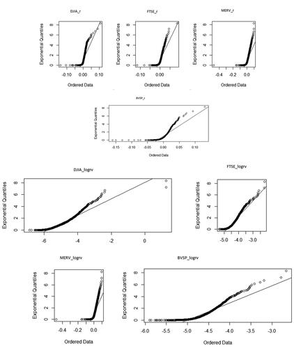
In terms of the graphical illustration, the QQ plot depicted in Figure 1 shows that there is an existence of heavy-tailed in the data series. The depiction of daily log-returns denoted as $r_t\mathrm{ }$ reveals an asymmetrical perspective of tail distribution, with notably greater deviations observed in the realm of extreme negative returns compared to the expectations of a Gaussian distribution. In contrast, for the ${\mathrm{\text{log}}\hspace{0.17em}\mathit{\text{RV}}}_{t\mathrm{ }},$ the Q-Q plot exhibits a right-skewed curve, implying that the predominance of extremes primarily lies within the right tail. The clear concavity in both daily and intraday returns is the strong signal of the heavy tailed presence in all data series, even though the intraday series displays stronger volatility periodicity patterns compared to the daily return series.

Figure 1. Q-Q Plot of daily returns, $r_t\mathrm{ }$ and intraday returns, ${\mathrm{\text{log}}\hspace{0.17em}\mathit{\text{RV}}}_t.$

4.2. Empirical analysis

In specific applications of EVT such as modeling exceptional occurrences in finance, the assumption of independence and identical distribution (iid) is appropriate. Because the EVT assumes iid observations, the original return series cannot be applied directly but must be filtered to make sure it follows an iid distribution. In this study, the standardized residuals filtered from GARCH, EGARCH and HAR model were tested by using the ARCH-LM, Q and Q2 statistics to make sure that it follows iid observations. The findings are displayed in Tables 3 and 4 which indicate that the ARCH-LM, Q, and Q2 tests yield insignificant results. This implies that the filtered standardized residuals series does not demonstrate serial dependence, in other words, free from serial correlation and conditional heteroskedasticity. Therefore, these filtered standardized residuals series are now assumed to be iid, making them suitable to be used in the EVT analysis. The filtered standardized residual series were estimated from January 1, 2014, to December 31, 2019, representing the non-crisis period, as well as the crisis years from January 1, 2020, to April 30, 2022.

Table 3. The heteroskedasticity and serial correlation test during the non-crisis period.

Stock Index	Model	ARCH-LM	Q	Q^2
DJIA	GARCH	0.137 [0.891]	6.899 [ 0.735]	9.89 [0.45]
	EGARCH	0.090 [0.928]	6.271 [0.792]	6.99 [0.73]
	FIEGARCH	0.087 [0.951]	6.130 [0.799]	6.00 [0.75]
	RV- G	0.109 [0.913]	36.511 [0.00]**	0.13 [1.00]
	RV-EG	0.125 [0.901]	28.365 [0.00]**	0.103 [1.00]
	RV-FIE	0.132 [0.882]	29.213 [0.00]**	0.11 [1.00]
	HAR	0.036 [0.972]	8.595 [0.571]	23.4 [0.01]**
	HAR-G	1.277 [0.208]	7.671 [0.661]	17.98 [0.06]
	HAR-EG	0.085 [0.933]	8.362 [0.594]	10.793 [0.37]
	HAR-FIE	0.078 [0.987]	8.024 [0.678]	9.85 [0.47]
FTSE100	GARCH	0.868 [0.386]	8.049 [0.624]	6.037 [0.812]
	EGARCH	0.424 [0.671]	10.374 [0.408]	1.847 [0.997]
	FIEGARCH	0.575 [0.502]	9.582 [0.495]	3.257 [0.7521]
	RV-G	0.453 [0.651]	289.83 [0.00]**	21.47 [0.02]*
	RV-EG	0.298 [0.766]	283.31 [0.00]**	21.34 [0.02]*
	RV-FIE	0.127 [0.785]	2793.2 [0.00]**	21.21 [0.00]*
	HAR	1.166 [0.249]	17.676 [0.061]	2.901 [0.984]
	HAR-G	1.860 [0.069]	20.597 [0.024]*	7.965 [0.632]
	HAR-EG	0.286 [0.776]	25.947 [0.00]**	4.416 [0.927]
	HAR-FIE	0.252 [0.786]	24.154 [0.00]**	3.566 [0.982]
BVSP	GARCH	0.666 [0.506]	3.403 [0.970]	3.983 [0.948]
	EGARCH	0.671 [0.502]	4.274 [0.934]	4.273 [0.934]
	FIEGARCH	0.684 [0.522]	4.551 [0.956]	4.524 [0.954]
	RV- G	1.563 [0.146]	12.226 [0.270]	13.88 [0.179]
	RV-EG	1.562 [0.146]	12.199 [0.272]	13.885 [0.178]
	RV-FIE	1.552 [0.141]	12.058 [0.275]	13.888 [0.177]
	HAR	1.223 [0.299]	7.113 [0.715]	16.31 [0.091]
	HAR-G	1.298 [0.257]	7.150 [0.711]	17.45 [0.065]
	HAR-EG	1.183 [0.325]	6.965 [0.729]	15.154 [0.127]
	HAR-FIE	1.152 [0.381]	6.825 [0.735]	15.112 [0.129]
MERVAL	GARCH	0.996 [0.319]	10.887 [0.366]	6.022 [0.813]
	EGARCH	0.873 [0.383]	10.642 [0.386]	8.931 [0.539]
	FIEGARCH	0.789 [0.254]	10.588 [0.389]	8.526 [0.556]
	RV-G	1.018 [0.309]	212.5 [0.00]**	17.225 [0.070]
	RV-EG	0.876 [0.382]	202.4 [0.00]**	15.937 [0.101]
	RV-FIE	0.855 [0.389]	201.2 [0.00]**	15.248 [0.125]
	HAR	1.614 [0.112]	11.09 [0.35]	21.02 [0.021]*
	HAR-G	0.545 [0.589]	12.30 [0.27]	18.45 [0.048]*
	HAR-EG	1.067 [0.291]	12.44 [0.26]	3.9127 [0.951]
	HAR-FIE	1.099 [0.282]	12.687 [0.26]	3.8251 [0.988]

Table 4. The heteroskedasticity and serial correlation test during the crisis period.

Model	Stock Index	ARCH-LM	Q	Q^2	Stock Index	ARCH-LM	Q	Q^2
GARCH	DJIA	1.190 [0.235]	13.328 [0.206]	3.627 [0.963]	BVSP	0.615 [0.539]	14.580 [0.148]	6.107 [0.806]
EGARCH		0.233 [0.816]	12.853 [0.232]	3.869 [0.953]		0.844 [0.399]	12.164 [0.274]	7.796 [0.649]
FIEGARCH		0.263 [0.805]	12.921 [0.204]	3.799 [0.968]		0.754 [0.421]	11.258 [0.280]	6.847 [0.795]
RV- G		1.515 [0.131]	69.817 [0.00]**	41.6 [0.00]**		0.188 [0.851]	21.415 [0.018]*	19.36 [0.04]*
RV-EG		1.529 [0.127]	46.851 [0.00]**	30.4 [0.00]**		0.238 [0.812]	21.984 [0.015]*	17.77 [0.059]
RV-FIE		1.623 [0.118]	45.267 [0.00]**	29.3 [0.00]**		0.197 [0.857]	20.256 [0.014]*	17.22 [0.051]
HAR		0.773 [0.452]	28.387 [0.00]**	16.2 [0.093]		0.413 [0.685]	12.223 [0.270]	9.252 [0.508]
HAR-G		0.400 [0.701]	26.597 [0.00]**	16.84 [0.078]		0.072 [0.944]	26.177 [0.00]**	6.107 [0.806]
HAR-EG		0.093 [0.929]	30.008 [0.00]**	10.62 [0.388]		0.102 [0.921]	14.982 [0.133]	6.632 [0.760]
HAR-FIE		0.088 [0.935]	29.877 [0.00]**	9.985 [0.392]		0.098 [0.935]	12.257 [0.087]	6.524 [0.779]
GARCH	FTSE100	0.542 [0.588]	19.503 [0.03]*	29.7 [0.00]**	MERVAL	0.345 [0.730]	6.014 [0.814]	15.88 [0.103]
EGARCH		1.293 [0.197]	18.888 [0.042]*	12.64 [0.245]		0.322 [0.747]	5.397 [0.863]	13.81 [0.182]
FIEGARCH		1.358 [0.188]	17.584 [0.052]	11.78 [0.251]		0.304 [0.758]	5.186 [0.875]	13.01 [0.199]
RV- G		4.07 [0.00]**	62.88 [0.00]**	34.0 [0.00]**		4.07 [0.00]**	62.88 [0.000]**	34.0 [0.00]**
RV-EG		1.982 [0.05]*	52.972 [0.00]**	31.28 [0.0]**		1.98 [0.05]*	52.97 [0.00]**	31.3 [0.00]**
RV-FIE		1.855 [0.05]*	48.741 [0.00]**	30.6 [0.00]**		1.788 [0.051]	48.7 [0.00]**	30.6 [0.00]**
HAR		0.218 [0.830]	34.892 [0.00]**	26.5 [0.00]**		0.948 [0.359]	7.1032 [0.716]	8.923 [0.539]
HAR-G		1.278 [0.237]	36.751 [0.00]**	26.3 [0.00]**		1.019 [0.342]	6.925 [0.732]	8.232 [0.606]
HAR-EG		0.268 [0.795]	37.168 [0.00]**	9.420 [0.493]		0.228 [0.826]	9.782 [0.460]	4.214 [0.937]
HAR-FIE		0.324 [0.705]	36.547 [0.00]**	8.579 [0.521]		0.197 [0.855]	8.547 [0.528]	3.887 [0.948]

The * and ** represent the significant value of p at 5% and 1% level, respectively.

In the second phase of data analysis utilizing EVT, the POT method was employed. This involved using the GPD distribution to estimate the tails of the data series. The in-sample filtered standardized residual series were estimated using conditional EVT models from January 1, 2014, to December 31, 2019, representing the non-crisis period, as well as the crisis years from January 1, 2020, to April 30, 2022. The threshold, u for each residual was determined by utilizing the following mean excess function (MEF) given by: (21) $$\mathit{\text{MEF}}\left(u\right)=\frac{{\sum }_{i=1}^n\left(X_i-u\right)}{{\sum }_{i=1}^n{I}_{(X_i>u)}},$$(21) where n represents the total number of in-sample observations. The selection of each threshold u occurs when the MEF plot reaches a satisfactory level of linearity. The range of possible values for all chosen u in this study were analyzed by using the R-programming code. The GPD parameters, ξ and ψ, were estimated for each selected u by using the maximum likelihood method. The resulting u, the number of exceedances (k), and the estimated parameters ξ and ψ are presented in Tables 5 and 6. The unconditional ${\mathit{\text{VaR}}}_q$ and ${\mathit{\text{ES}}}_q$ are calculated by using the formula given in Equations (9)(9) $$\mathit{\text{Va}}{R}_q=x_q=u+\frac{\psi }{\xi }\left[{\left(\frac{1-q}{k/n}\right)}^{-\xi }-1\right].$$(9) and (11)(11) $$E{S}_q=\frac{\mathit{\text{Va}}{R}_q}{1-\xi }+\frac{\psi -\xi u}{1-\xi }.$$(11) at 95% and 99% confidence level.

Table 5. The GPD parameter estimates during non-crisis period (2014–2019).

Risk Model	Index	ξ	ψ	VaR		ES		Index	ξ	ψ	VaR		ES
				0.95	0.99	0.95	0.99				0.95	0.99	0.95	0.99
GARCH	DJIA	0.232**	0.004**	0.012	0.019	0.017	0.026	BVSP	0.139**	0.210**	0.44	0.809	0.677	1.105
EGARCH		0.212*	0.004**	0.012	0.019	0.017	0.026		0.141*	0.209*	0.44	0.808	0.677	1.105
FIEGARCH		0.212*	0.004**	0.012	0.019	0.017	0.026		0.117**	0.219**	0.431	0.81	0.674	1.103
RV- G		0.846**	0.078**	0.467	0.689	0.886	2.325		0.139**	0.210**	0.44	0.809	0.677	1.105
RV-EG		0.902*	0.071**	0.465	0.676	1.061	3.221		0.141**	0.209**	0.44	0.808	0.677	1.105
RV-FIE		0.916*	0.070**	0.464	0.673	1.139	3.62		0.117*	0.219**	0.431	0.81	0.674	1.103
HAR		−0.665*	0.368**	0.347	0.41	0.385	0.423		−0.573*	0.270*	0.438	0.595	0.533	0.633
HAR-G		−0.70**	0.382**	0.371	0.429	0.407	0.441		−0.758*	0.346*	0.475	0.622	0.565	0.648
HAR-EG		−0.94**	0.513**	0.379	0.416	0.402	0.421		−0.489*	0.254**	0.448	0.611	0.546	0.655
HAR-FIE		−0.66**	0.362**	0.31	0.372	0.348	0.386		−0.67**	0.307**	0.456	0.597	0.542	0.626
GARCH	FTSE	−0.230*	0.007**	0.014	0.024	0.02	0.028	MERVAL	−0.087*	0.013**	0.036	0.056	0.048	0.066
EGARCH		−0.276*	0.008**	0.014	0.024	0.02	0.029		−0.077*	0.013**	0.037	0.056	0.049	0.067
FIEGARCH		−0.250*	0.007**	0.014	0.024	0.02	0.028		−0.057*	0.012**	0.037	0.056	0.048	0.066
RV- G		0.197**	0.166**	0.53	0.831	0.728	1.103		−0.096*	0.261*	0.594	0.988	0.835	1.194
RV-EG		0.218*	0.159*	0.532	0.825	0.726	1.1		−0.136*	0.280*	0.588	1	0.839	1.202
RV-FIE		0.219**	0.159*	0.53	0.821	0.723	1.096		−0.121*	0.274*	0.582	0.99	0.831	1.195
HAR		−1.551*	0.086*	0.441	0.483	0.469	0.485		−0.785*	0.432*	0.693	0.866	0.799	0.896
HAR-G		0.095*	0.019*	0.485	0.527	0.511	0.558		−0.600*	0.355**	0.736	0.92	0.848	0.963
HAR-EG		−2.279*	0.326**	0.495	0.539	0.526	0.539		−0.57**	0.351**	0.612	0.816	0.735	0.866
HAR-FIE		−1.217*	0.253**	0.398	0.45	0.431	0.454		−0.78**	0.431**	0.664	0.838	0.771	0.869

The * and ** represent the significant value of p at 5% and 1% level, respectively.

Table 6. The GPD parameter estimates during crisis period (2020–2022).

Risk Model	Index	ξ	ψ	VaR		ES		Index	ξ	ψ	VaR		ES
				0.95	0.99	0.95	0.99				0.95	0.99	0.95	0.99
GARCH	DJIA	0.394**	0.008**	0.023	0.051	0.044	0.09	BVSP	0.256*	0.010**	0.029	0.056	0.047	0.084
EGARCH		0.366*	0.008**	0.024	0.051	0.044	0.087		0.300**	0.009*	0.029	0.056	0.048	0.087
FIEGARCH		0.366*	0.008**	0.024	0.051	0.044	0.087		0.326**	0.009**	0.029	0.056	0.048	0.089
RV- G		−0.128**	0.556**	1.071	1.683	1.444	1.986		−0.072*	0.152*	0.447	0.659	0.578	0.775
RV-EG		−0.074*	0.528**	1.093	1.772	1.51	2.142		−0.071*	0.152**	0.447	0.66	0.578	0.777
RV-FIE		−0.094*	0.547**	1.093	1.772	1.51	2.142		−0.058*	0.147**	0.439	0.651	0.57	0.77
HAR		−0.492*	0.992**	0.921	1.178	1.076	1.248		−1.072*	0.249**	0.31	0.34	0.329	0.344
HAR-G		−0.667*	1.312**	0.951	1.131	1.06	1.168		−2.231*	0.358**	0.317	0.327	0.324	0.327
HAR-EG		−0.74**	1.301**	0.95	1.088	1.035	1.114		−2.126*	0.344**	0.291	0.302	0.299	0.302
HAR-FIE		−0.43**	0.916**	0.996	1.286	1.171	1.373		−2.696*	0.479**	0.335	0.342	0.34	0.342
GARCH	FTSE	0.240**	0.007*	0.024	0.042	0.036	0.059	MERVAL	−0.081*	0.021*	0.047	0.076	0.064	0.091
EGARCH		0.216**	0.007*	0.022	0.04	0.034	0.056		−0.140*	0.023**	0.048	0.077	0.065	0.09
FIEGARCH		0.168**	0.008*	0.022	0.04	0.034	0.055		−0.11**	0.022**	0.049	0.077	0.066	0.092
RV- G		−0.147*	0.576*	0.952	1.654	1.379	1.99		−0.152*	0.267*	0.575	0.888	0.765	1.036
RV-EG		−0.096*	0.515**	0.903	1.592	1.324	1.954		−0.145*	0.266**	0.571	0.886	0.762	1.038
RV-FIE		−0.092*	0.506**	0.899	1.582	1.317	1.943		−0.13**	0.260**	0.586	0.905	0.781	1.062
HAR		−0.037*	0.300**	0.645	1.082	0.914	1.336		−0.197*	0.226*	0.424	0.635	0.552	0.728
HAR-G		0.811**	0.109**	0.671	2.547	3.668	13.604		0.189*	0.141**	0.407	0.797	0.663	1.144
HAR-EG		−0.045*	0.305**	0.713	1.147	0.98	1.395		0.046**	0.169**	0.497	0.807	0.691	1.016
HAR-FIE		−0.039*	0.302**	0.713	1.15	0.983	1.404		−0.213*	0.232**	0.445	0.653	0.571	0.742

The * and ** represent the significant value of p at 5% and 1% level, respectively.

4.3. Backtesting VaR

The assessment of various volatility models for daily and intraday returns, in both normal and crisis times, has relied on the utilization of the violation ratio (VR) as an evaluative measure. According to the guidelines provided by Danielsson (2011), a VR value within the range of [0.8,1.2] indicates a good forecast. However, the VR values outside this range suggest an imprecise or not good model. Nevertheless, the VR within [0.5,0.8] or [1.2,1.5] is still acceptable. Based on the results presented in Table 7, most of the HAR-type models combined with EVT are precise and acceptable to be used in the VaR forecast. Next, Tables 8 and 9 reveal the VaR backtesting results by using UC and CC test. Based on the result, during normal and crisis period, all high-frequency HAR models accepted the null hypothesis at a 5% significance level which implies that the corresponding high-frequency VaR models have adequate forecasting ability. The low-frequency models of GARCH-EVT and EGARCH-EVT reject the null hypothesis at 5% significance level which means the low-frequency models combined with EVT are not suitable to forecast the VaR during both normal and crisis period.

Table 7. The VaR violation ratios of the Conditional-EVT Model.

Stock Index	Low-frequency	Normal	Crisis	High-frequency	Normal	Crisis
DJIA	G-EVT	10.45	9.63	RV-G-EVT	9.88	11.11
	EG-EVT	10.86	11.03	RV-EG-EVT	9.79	9.55
	FIEGARCH	10.53		RV-FIEG-EVT	9.71	9.55
				HAR-EVT	1.51	1.05
				HAR-G-EVT	2.26	2.00
				HAR-EG-EVT	1.89	4.00
				HAR-FIEG-EVT	8.00	2.00
FTSE	G-EVT	10.95	10.56	RV-G-EVT	9.68	11.59
	EG-EVT	10.48	10.87	RV-EG-EVT	10.00	10.56
	FIEGARCH	10.48	11.67	RV-FIEG-EVT	10.00	10.00
				HAR-EVT	1.13	2.00
				HAR-G-EVT	0.97	4.00
				HAR-EG-EVT	1.61	6.00
				HAR-FIEG-EVT	9.43	2.00
BVSP	G-EVT	0.74	0.66	RV-G-EVT	12.43	9.22
	EG-EVT	10.54	10.37	RV-EG-EVT	10.70	10.78
	FIEGARCH	10.78	11.11	RV-FIEG-EVT	10.70	11.77
				HAR-EVT	1.13	0.69
				HAR-G-EVT	0.76	5.52
				HAR-EG-EVT	1.51	6.00
				HAR-FIEG-EVT	0.38	6.00
MERVAL	G-EVT	10.08	10.62	RV-G-EVT	9.60	11.61
	EG-EVT	10.08	9.88	RV-EG-EVT	9.68	11.28
	FIEGARCH	10.24	10.53	RV-FIEG-EVT	3.17	11.08
				HAR-EVT	0.38	2.00
				HAR-G-EVT	0.76	1.43
				HAR-EG-EVT	0.38	2.14
				HAR-FIEG-EVT	1.51	2.14

The bold figure represents the performance is acceptable and good.

Table 8. The UC and CC test statistics of the Conditional-EVT Model during normal period.

Index	Low-freq	LRUC		LRCC		High-freq	LRUC		LRCC
		Stat	p	Stat	p		Stat	p	Stat	p
DJIA	G-EVT	436.45	0	438.03	0	RV-G-EVT	394.76	0	394.77	0
	EG-EVT	467.21	0	468.71	0	RV-EG-EVT	388.94	0	388.94	0
	FIEG-EVT	442.53	0	450.23	0	RV-FIEG-EVT	383.15	0	383.19	0
						HAR-EVT	0.63	0.43	0.63	.73
						HAR-G-EVT	3.33	0.07	3.33	.19
						HAR-EG-EVT	1.76	0.19	1.76	.42
						HAR-FIE-EVT	79.36	0	79.39	0
FTSE	G-EVT	460.51	0	461.21	0	RV-G-EVT	395.2	0	395.2	0
	EG-EVT	454.41	0	454.42	0	RV-EG-EVT	418.5	0	422.58	0
	FIEG-EVT	448.35	0	450.57	0	RV-FIEG-EVT	400.98	0	402.02	0
						HAR-EVT	0.05	0.83	0.05	.98
						HAR-G-EVT	0	0.95	0	1
						HAR-EG-EVT	1.04	0.31	1.83	0.4
						HAR-FIE-EVT	2.011	0.156	2.017	.365
BVSP	G-EVT	442.53	0	442.55	0	RV-G-EVT	591.75	0	592.59	0
	EG-EVT	460.99	0	469.58	0	RV-EG-EVT	454.8	0	464.89	0
	FIEG-EVT	454.8	0	459.47	0	RV-FIEG-EVT	454.8	0	459.47	0
						HAR-EVT	0.05	0.83	0.05	.98
						HAR-G-EVT	0.18	0.67	0.18	.91
						HAR-EG-EVT	0.63	0.43	2.18	.34
						HAR-FIE-EVT	1.404	0.24	1.41	.494
MERV	G-EVT	424.41	0	468.68	0	RV-G-EVT	389.46	0	421.49	0
	EG-EVT	424.41	0	424.41	0	RV-EG-EVT	395.2	0	427.67	0
	FIEG-EVT	436.31	0	481.48	0	RV-FIEG-EVT	40.88	0	46.15	0
						HAR-EVT	1.4	0.24	1.41	0.49
						HAR-G-EVT	0.18	0.67	0.18	.91
						HAR-EG-EVT	1.4	0.24	1.41	.49
						HAR-FIE-EVT	1.404	0.24	1.41	.494

The bold figures mean the null hypothesis is accepted based on p-value above 5% and critical values less than 3.841 which implies that the corresponding VaR model has adequate forecasting ability.

Table 9. The UC and CC test statistics of the Conditional-EVT Model during crisis period.

Index	Low-freq	LRUC		LRCC		High-freq	LRUC		LRCC
		Stat	p	Stat	p		Stat	p	Stat	p
DJIA	G-EVT	377.39	0	379.82	0	RV-G-EVT	486.06	0	487.2	0
	EG-EVT	479.75	0	484.65	0	RV-EG-EVT	371.67	0	372.73	0
	FIEG-EVT	442.53	0	447.125	0	RV-FIEG-EVT	371.667	0	372.223	0
						HAR-EVT	0	0.96	0.02	.99
						HAR-G-EVT	0.41	0.52	0.46	.8
						HAR-EG-EVT	2.8	0.1	2.81	.25
						HAR-FIE-EVT	0.413	0.52	0.456	.796
FTSE	G-EVT	460.51	0	463.94	0	RV-G-EVT	542.66	0	544.34	0
	EG-EVT	485.21	0	485.48	0	RV-EG-EVT	460.51	0	460.85	0
	FIEG-EVT	549.2	0	551.479	0	RV-FIEG-EVT	418.504	0	419.791	0
						HAR-EVT	0.41	0.52	0.46	.8
						HAR-G-EVT	2.8	0.1	2.81	.25
						HAR-EG-EVT	6.48	0.01	6.5	.04
						HAR-FIE-EVT	0.413	0.52	0.456	.796
BVSP	G-EVT	430.39	0	432.31	0	RV-G-EVT	349.1	0	373.45	0
	EG-EVT	424.37	0	426.29	0	RV-EG-EVT	460.99	0	466.66	0
	FIEG-EVT	486.06	0	486.932	0	RV-FIEG-EVT	537.818	0	541.88	0
						HAR-EVT	0.16	0.69	0.18	.92
						HAR-G-EVT	15.92	0	18.55	0
						HAR-EG-EVT	6.48	0.01	6.48	.04
						HAR-FIE-EVT	29.26	0	29.26	0
MERV	G-EVT	448.65	0	448.79	0	RV-G-EVT	524.68	0	524.73	0
	EG-EVT	394.76	0	398.2	0	RV-EG-EVT	498.8	0	503.46	0
	FIEG-EVT	442.53	0	448.275	0	RV-FIEG-EVT	459.951	0	460.297	0
						HAR-EVT	0.04	0.84	0.46	.8
						HAR-G-EVT	0.24	0.62	0.24	.89
						HAR-EG-EVT	1.47	0.23	1.47	.48
						HAR-FIE-EVT	1.471	0.225	1.471	.479

The bold figure means the null hypothesis is accepted based on p-value above 5% and critical values of 3.841 which implies that the corresponding VaR model has adequate forecasting ability.

Since HAR type-models passed all the first stage backtesting procedure by using the statistical test of the UC and CC test, these models will be tested again by using the RLF and FLF lost function on the VaR accuracy. In Table 10, during the normal period, the HAR-EVT model exhibits better performance than alternative HAR models in forecasting VaR. Conversely, in the period of crisis, the HAR-EGARCH-EVT model demonstrated the most superior performance by achieving the lowest values for both the RLF and FLF loss functions.

Table 10. The RLF and FLF values.

Stock Index	Models	Non-crisis		Crisis
		RLF	FLF	RLF	FLF
DJIA	HAR-EVT	0.0706	0.1740	0.1900	0.3460
	HAR-G-EVT	0.0002	0.2550	0.1630	0.3340
	HAR-EG-EVT	0.0087	0.2300	0.1530	0.3130
	HAR-FIEG-EVT	0.0797	0.1920	0.0796	0.0782
FTSE	HAR-EVT	0.0906	0.1750	0.0334	0.0320
	HAR-G-EVT	0.0901	0.1780	0.0314	0.0300
	HAR-EG-EVT	0.0962	0.1830	0.0285	0.0270
	HAR-FIEG-EVT	0.1140	0.2020	0.6010	0.5990
BVSP	HAR-EVT	0.0011	0.0000	0.2970	0.3470
	HAR-G-EVT	0.0011	0.2350	0.1560	0.2240
	HAR-EG-EVT	0.0000	0.0000	0.0557	0.0549
	HAR-FIEG-EVT	0.0016	0.2270	0.1460	0.2070
MERVAL	HAR-EVT	0.0503	0.1530	0.0431	0.1050
	HAR-G-EVT	0.0543	0.1510	0.0391	0.1000
	HAR-EG-EVT	0.0006	0.0046	0.0400	0.1020
	HAR-FIEG-EVT	0.0596	0.1760	0.0823	0.1640

4.4. Backtesting ES

Based on the results obtained in Table 11, the low-frequency conditional EVT models have produced a larger value of GB, which indicates that there are severe breaches in the data. Additionally, the ES estimate is inaccurate based on the significant p-value. If the p-value is significant, the $H_0$ is rejected, suggesting that the low-frequency conditional EVT models are not adequate for accurately estimating the ES during a non-crisis period. However, during the crisis period, it shows that the low-frequency conditional EVT models are accurate to be used in estimating the ES. The high-frequency conditional EVT models generate lower values of the GB which suggests that the actual losses are closer to the expected losses calculated from the ES estimate, indicating that the ES estimate is more accurate. The bold figure shows the accurate ES measure by using the HAR-type models.

Table 11. The backtesting procedure of expected shortfall.

Stock Index	Risk Model	Non-crisis			Crisis
		GB	z	p	GB	z	p
DJIA	G-EVT	43.37	95.47	0	8.31	0.47	.64
	EG-EVT	43.37	95.47	0	8.31	0.48	.63
	FIEG-EVT	43.37	95.47	0	8.31	0.47	.64
	RV-G-EVT	2	−231.14	0	0	−64.55	0
	RV-EG-EVT	2	−231.14	0	0	−64.55	0
	RV-FIEG-EVT	2	−231.14	0	0	−64.55	0
	HAR-EVT	1.84	0.29	.77	0	−5.53	0
	HAR-G-EVT	1.84	0.29	.77	0	−5.53	0
	HAR-E-EVT	1.84	0.29	.77	0	−5.53	0
	HAR-F-EVT	1.95	1.21	.23	0	−5.53	0
FTSE	G-EVT	27	−36.53	0	7.71	−5.22	0
	EG-EVT	23.08	−67.47	0	11.28	22.95	0
	FIEG-EVT	23.88	−61.19	0	10.74	18.65	0
	RV-G-EVT	4.62	−211.83	0	0	−65.73	0
	RV-EG-EVT	4.62	−211.84	0	0	−65.73	0
	RV-FIEG-EVT	4.62	−211.86	0	0	−65.73	0
	HAR-EVT	1.83	0.45	.63	0	−5.72	0
	HAR-G-EVT	1.84	0.46	.64	0	−5.72	0
	HAR-E-EVT	1.83	0.46	.64	0	−5.72	0
	HAR-F-EVT	1.83	0.46	.64	0	−5.72	0
BVSP	G-EVT	6.8	−188.27	0	9.58	11.07	0
	EG-EVT	6.81	−188.26	0	9.17	7.87	0
	FIEG-EVT	7.73	−180.95	0	9.17	7.84	0
	RV-G-EVT	1.99	−226.31	0	0.99	−56.33	0
	RV-EG-EVT	1.99	−226.31	0	0.99	−56.33	0
	RV-FIE-EVT	1.99	−226.31	0	0.99	−56.33	0
	HAR-EVT	0.99	−6.18	0	0	−5.72	0
	HAR-G-EVT	0.99	−6.17	0	0	−5.72	0
	HAR-E-EVT	1	−6.15	0	−0.81	−12.09	0
	HAR-F-EVT	0.99	−6.16	0	0	−5.72	0

The significance level used in this analysis is 5% significance level. The bold figures show that the ES models are accurate.

5. Discussion

The result provided in the previous section shows that for VaR forecast, the result of the the first stage basktesting procedure reveal that the HAR-EVT typed-models outperformed other risk models that apply the GARCH and RV specification with EVT. Furthermore, the result from the second stage of the bactesting procedure shown that among all hybrid version of HAR-EVT models, the HAR-EGARCH-EVT model exhibits superior performance in forecasting the VaR during both normal and crisis period as summarized in Table 12.

Table 12. The best performance models based on the VaR forecast.

Total		Non-crisis	Crisis
	HAR-EVT	2	0
	HAR-G-EVT	2	2
	HAR-EG-EVT	4	4
	HAR-FIEG-EVT	0	1

The bold figure represents the best performing model.

On the other hand, based on the ES forecast, during the non-crisis period, based on samples of DJIA and FTSE indices, the result shows insignificant values, suggesting that the HAR specification models combined with EVT are adequate in estimating the ES during the non-crisis period. This result is consistent with the VaR forecast result where HAR-EVT typed models outperformed other models in estimating the risk. However, during the crisis period, GARCH-EVT, EGARCH-EVT and FIEGARCH-EVT show insignificant values and suitable to estimate expected shortfall with higher severity of the breach. There is no breach detected in the HAR-EVT typed models during the crisis period. The result is not consistent with the VaR forecast. The reason might be because the small sample of sizes used to forecast the ES during the crisis period make it difficult to detect the number of breaches by using HAR specification that based on monthly and weekly data.

This research findings also provide practitioners and policymakers with the best volatility forecast model to be used during any extreme market sudden event. There are unique features possessed by high-frequency data but lacking in low-frequency data which make it more suitable to be used in the current volatility estimation model. The findings of this research study are also beneficial to market participants, especially those who engage in high-frequency trading to utilize the RV and HAR models as well the application of the EVT model to measure the potential risks and detect any vulnerabilities in financial systems especially during a sudden market crash. In the context of economic sustainability, the research findings help to provide an accurate risk model which will help in reducing the unanticipated risk in the stock market and maintain the stability of financial systems thus sustaining the global economics. Furthermore, this research study will provide insights into the superiority of high-frequency data in comparison to low-frequency data. An increase in high-frequency research has the potential to propel future technological advancements, particularly in artificial intelligence (AI) and machine learning. This surge could notably bolster the processing of high-frequency data by streamlining and automating the analysis procedures. Larger data volumes can be handled in a more efficient and precise manner, obtaining more valuable information and trends faster than traditional methods. Over time, the prospect of diminishing the overall cost associated with processing high-frequency data is highly probable. This reduction could make data processing more accessible and affordable for smaller-scale and individual investors.

6. Conclusion

The utilization of daily returns for risk prediction through EVT has experienced a significant transformation, transitioning from the traditional EVT approach to the more advanced hybrid method called a conditional EVT model. The research on how the conditional EVT outperforms other models is still ongoing until 2023 with different hybrid methods among all available risk models. The emergence of high-frequency data contributes to another area of research on the efficiency of the low-frequency conditional EVT models compared to the high-frequency conditional EVT models. Researchers discovered that, for the most part, when high-frequency data was compared, the conditional EVT exhibited superior performance as discussed earlier in the literature review. Many investigations have been carried out to validate the advantages of integrating the RV specification into a hybrid model alongside the EVT method. The result from this study highlighted that high-frequency conditional EVT models can surpass low-frequency conditional EVT models in risk forecasting the VaR and ES. The summary result suggests that all models that combined the HAR specification with EVT have passed all first stage VaR backtesting procedure during both non-crisis and crisis periods which concludes that the combination of the HAR model and EVT approach can produce precise predictions of market risk, especially during sudden market crashes such as the COVID-19 pandemic period.

This research study contributes to the theoretical and practical implications in terms of its findings. Theoretically, this study differs from previous research and contributes to current literature on the forecasting ability of risk models by concentrating on the hybrid model of long-memory models (FIEGARCH, RV-FIEGARCH and HAR-FIEGARCH) for various types of data (daily and intraday returns) with the EVT approach. This research filled the gap by introducing the exponential variant of the fractionally integrated RV model, known as the RV-FIEGARCH model that not only encompasses the long-memory aspect but also accounts for the asymmetric effects in the return series. In addition to this, the research study also implemented the HAR framework, by utilizing the daily, weekly, and monthly data within the exponential fractionally integrated RV model, referred to as the HAR-RV-FIEGARCH model, to assess its potential in enhancing the accuracy of forecasting particularly during periods of crisis and stability. The result of this research verifies that the HAR specifications combined with the EVT approach including the HAR-FIEGARCH-EVT outperformed other risk models during periods of for both developed and emerging markets.

Disclosure statement

No potential conflict of interest was reported by the author(s).

Additional information

Notes on contributors

Nor Azliana Aridi

Nor Azliana Aridi is a senior lecturer at the Faculty of Management, Multimedia University (MMU) in Cyberjaya, Malaysia. She specializes in teaching Mathematics and Statistics to both foundation and undergraduate students. She holds a bachelor’s degree in mathematical science from International Islamic University Malaysia (IIUM) obtained in 2007 and a master’s degree in mathematics from the National University of Malaysia (UKM) obtained in 2009. Recently in March 2024, she completed her PhD in Management, specializing in Financial Econometrics at MMU. Nor Azliana is an active researcher, frequently presenting at international conferences and publishing journal papers. Her research interests focus on financial econometrics, and she is proficient in using various statistical software, including R, EViews, OxMetrics, and SPSS. Additionally, she has been successful in securing internal research grants to support her work. In her role at MMU, she also takes on administrative and management tasks, contributing to her versatility and well-rounded skill set within the academic community.

Tan Siow Hooi

Tan Siow Hooi is an Associate Professor at Faculty of Management, Multimedia University. She received her PhD degree majoring in Financial Economics from Faculty of Economics and Management, Universiti Putra Malaysia. She has many years of experience teaching a variety of economics and econometrics courses at both the undergraduate and graduate levels. Her research profile is interdisciplinary. She has published widely on a number of issues in the field of behavioural finance, tourism and cultural heritage, as well as environmental responsibility. Topics of interest in recent years include predictability of financial markets, technology for elderly, placed-based education and heritage. Her articles have been published in Web of Science SSCI indexed journals, including The North American Journal of Economics and Finance, Journal of Behavioural Finance, Journal of Environmental Management, Annals of Tourism Research, Current Issues in Tourism, Tourism Management, Tourism Economics, among many others. She has extensively used a wide range of statistical packages, which include but are not limited to EViews, STATA, Matlab, R, SPSS, AMOS, Excel and Google Spreadsheet in her research works as well as in statistical laboratory for the teaching of multivariate data analysis, time series analysis and forecasting, and econometrics. She is a HRDF-certified trainer for Train-the-Trainer (TTT) and Alibaba Certified Global E-Commerce Talent (GET).

Chin Wen Cheong

Chin Wen Cheong is affiliated to Xiamen University, Malaysia. Chin Wen Cheong is currently providing services as Associate Professor in School of Mathematics and Physics. He obtained his bachelor’s degree in Physics from University of Malaya, Malaysia (1998), master’s degree in Applied Statistics from University of Putra Malaysia, Malaysia (2003) and Ph. D Degree (Statistics) from National University Malaysia, Malaysia (2011). He has authored and co-authored multiple peer-reviewed scientific papers and presented works at many national and international conferences. His contributions have acclaimed recognition from honourable subject experts around the world. Chin Wen Cheong is actively associated with different societies and academies. His academic career is decorated with several reputed awards and funding. His research interests include time series and risk management.

References

- Altun, E., & Tatlidil, H. (2015). A comparison of extreme value theory with heavy - tailed distributions in modeling daily VaR. Journal of Finance and Investment Analysis, 4, 1–5.
- Balkema, A. A., & Haan, L. D. (1974). Residual life time at great age. The Annals of Probability, 2(5), 792–804. https://doi.org/10.1214/aop/1176996548
- Basel Committee on Banking Supervision. (1996). Supervisory framework for the use of “backtesting” in. conjunction with the internal models approach to market risk capital requirements. Bank for International Settlements, Basle, Report nr. 22, http://www.bis.org
- Basuony, M. A., Bouaddi, M., Ali, H., & EmadEldeen, R. (2022). The effect of COVID-19 pandemic on global stock markets: Return, volatility, and bad state probability dynamics. Journal of Public Affairs, 22(S1), e2761. https://doi.org/10.1002/pa.2761
- Bee, M., Dupuis, D. J., & Trapin, L. (2016). Realizing the extremes: Estimation of tail-risk measures from a high-frequency perspective. Journal of Empirical Finance, 36, 86–99.
- Cheong, C. H., Cherng, L. M., & Yap, G. L. C. (2016). Heterogeneous market hypothesis evaluations using various jump-robust realized volatility. Romanian Journal of Economic Forecasting, XIX(4), 50–64.
- Christoffersen, P. F. (1998). Evaluating interval forecasts. International Economic Review, 39(4), 841–862. https://doi.org/10.2307/2527341
- Costanzino, N., & Curran, M. (2015). Backtesting general spectral risk measures with application to expected shortfall. Available at SSRN 2514403.
- Dacorogna, M., Mller, U., Olsen, R., & Pictet, O. (2001). Defining efficiency in heterogeneous markets. Quantitative Finance, 1(2), 198–201. https://doi.org/10.1088/1469-7688/1/2/602
- Danielsson, J. (2011). Financial risk forecasting: The theory and practice of forecasting market risk with implementation in R and Matlab. John Wiley & Sons.
- Djuraskovic, O. (2023). Big data statistics 2023: How much data is in the world? First Site Guide. https://firstsiteguide.com/big-data-stats/
- Embrechts, P., Klüppelberg, C., & Mikosch, T. (2013). Modelling extremal events: for insurance and finance (Vol. 33). Springer Science & Business Media.
- Fama, E. (1965). The behavior of stock-market prices. The Journal of Business, 38(1), 34–105. https://doi.org/10.1086/294743
- Huang, Z., Liu, H., & Wang, T. (2016). Modeling long memory volatility using realized measures of volatility: A realized HAR GARCH model. Economic Modelling, 52(Part B), 812–821. https://doi.org/10.1016/j.econmod.2015.10.018
- Hui, E. C. M., & Chan, K. K. K. (2022). How does Covid-19 affect global equity markets? Financial Innovation, 8(1), 25. https://doi.org/10.1186/s40854-021-00330-5
- Jafry, N. H. A., Razak, R. A., & Ismail, N. (2020). Dependence measure of five-minutes returns compared to daily returns using static and dynamic copulas. Sains Malaysiana, 49(8), 2023–2034.
- James, R., & Leung, J. W. Y. (2023). Forecasting financial risk using quantile random forests. Available at SSRN 4324603.
- Jin, F., Li, J., & Li, G. (2022). Modeling the linkages between Bitcoin, gold, dollar, crude oil, and stock markets: A GARCH-EVT-copula approach. Discrete Dynamics in Nature and Society, 2022, 1–10. https://doi.org/10.1155/2022/8901180
- Kickbusch, I., Leung, G. M., Bhutta, Z. A., Matsoso, M. P., Ihekweazu, C., & Abbasi, K. (2020). Covid-19: How a virus is turning the world upside down. BMJ, 369, m1336. https://doi.org/10.1136/bmj.m1336
- Kupiec, P. H. (1995). Techniques for verifying the accuracy of risk measurement models. The Journal of Derivatives, 3(2), 73–84. https://doi.org/10.3905/jod.1995.407942
- Liu, G., Yu, C. P., Shiu, S. N., & Shih, I. T. (2022). The efficient market hypothesis and the fractal market hypothesis: Interfluves, fusions, and evolutions. SAGE Open, 12(1), 215824402210821. https://doi.org/10.1177/21582440221082137
- Lopez, J. A. (1998). Methods for evaluating value-at-risk estimates. Economic Policy Review, 4(3), 119–991124.
- Louzis, D. P., Sissinis, S. X., & Refenes, A. (2007). Stock index Value-at Risk forecasting: A realized volatility extreme value theory approach. Economics Bulletin, 32(1), 981–991.
- Lyócsa, S., Molnár, P., & Výrost, T. (2021). Stock market volatility forecasting: Do we need high-frequency data? International Journal of Forecasting, 37(3), 1092–1110. https://doi.org/10.1016/j.ijforecast.2020.12.001
- Maaz, K., Mrestyal, K., & Muhammad, I. (2023). Estimating value-at-risk and expected shortfall of metal commodities: Application of GARCH-EVT method. Journal of Risk Management in Financial Institutions, Henry Stewart Publications, 16(2), 189–199.
- Mcneil, A. J., & Frey, R. (2000). Estimation of tail-related risk measures for heteroscedastic financial time series: an extreme value approach. Journal of Empirical Finance, 7(3-4), 271–300. https://doi.org/10.1016/S0927-5398(00)00012-8
- Omari, C., Mundia, S., & Ngina, I. (2020). Forecasting value-at-risk of financial markets under the global pandemic of COVID-19 using conditional extreme value theory. Journal of Mathematical Finance, 10(04), 569–597. https://doi.org/10.4236/jmf.2020.104034
- Paul, S., & Sharma, P. (2018). Quantile forecasts using the realized GARCH-EVT approach. Studies in Economics and Finance, 35(4), 481–504. https://doi.org/10.1108/SEF-09-2016-0236
- Pickands, J. (1975). Statistical inference using extreme order statistics. The Annals of Statistics, 3(1), 119–131.
- Rakshit, B., & Neog, Y. (2022). Effects of the COVID-19 pandemic on stock market returns and volatilities: evidence from selected emerging economies. Studies in Economics and Finance, 39(4), 549–571. https://doi.org/10.1108/SEF-09-2020-0389
- Roy, A. (2022). Efficacy of GARCH-EVT model in intraday risk management: Evidence from severely pandemic-affected countries. Global Business Review, 097215092211048. https://doi.org/10.1177/09721509221104848
- Sarma, M., Thomas, S., & Shah, A. (2003). Selection of value-at-risk models. Journal of Forecasting, 22(4), 337–358. https://doi.org/10.1002/for.868
- Sojka, B. B. (2015). Daily VaR forecasts with realized volatility and GARCH Models. Argumenta Oeconomica, 34(1), 157–173.
- Soltane, H. B., Karaa, A., & Bellalah, M. (2012). Conditional VaR using GARCH-EVT approach: forecasting volatility in Tunisian financial market. Journal of Computations & Modelling, 2(2), 95–115.
- Tabasi, H., Yousefi, V., Tamošaitienė, J., & Ghasemi, F. (2019). Estimating conditional value at risk in the Tehran stock exchange based on the extreme value theory using GARCH models. Administrative Sciences, 9(2), 40. https://doi.org/10.3390/admsci9020040
- Tao, Q., Wei, Y., Liu, J., & Zhang, T. (2018). Modeling and forecasting multifractal volatility established upon the heterogeneous market hypothesis. International Review of Economics & Finance, 54, 143–153. https://doi.org/10.1016/j.iref.2017.08.003
- Ullah, S. (2022). Impact of COVID-19 pandemic on financial markets: A global perspective. Journal of the Knowledge Economy, 14(2), 982–1003. https://doi.org/10.1007/s13132-022-00970-7
- Watanabe, T. (2012). Quantile forecasts of financial returns using realized Garch models. Japanese Economic Review, 63(1), 68–80. https://doi.org/10.1111/j.1468-5876.2011.00548.x
- Youssef, M., Belkacem, L., & Mokni, K. (2015). Value-at-risk estimation of energy commodities: A long-memory GARCH–EVT approach. Energy Economics, 51, 99–110. https://doi.org/10.1016/j.eneco.2015.06.010
- Zahid, M., Iqbal, F., Raziq, A., & Sheikh, N. (2022). Modeling and forecasting the realized volatility of bitcoin using realized HAR-GARCH-type models with jumps and inverse leverage effect. Sains Malaysiana, 51(3), 929–942. https://doi.org/10.17576/jsm-2022-5103-25
- Zhang, Z., & Zhang, H. K. (2016). The dynamics of precious metal markets VaR: A GARCH-EVT approach. Journal of Commodity Markets, 4(1), 14–27. https://doi.org/10.1016/j.jcomm.2016.10.001
- Zhao, J., Cui, L., Liu, W., & Zhang, Q. (2023). Extreme risk spillover effects of international oil prices on the Chinese stock market: A GARCH-EVT-Copula-CoVaR approach. Resources Policy, 86(Part B), 104142. https://doi.org/10.1016/j.resourpol.2023.104142