
 ?Mathematical formulae have been encoded as MathML and are displayed in this HTML version using MathJax in order to improve their display. Uncheck the box to turn MathJax off. This feature requires Javascript. Click on a formula to zoom.
Abstract
We derive a priori error estimates for the standard Galerkin and streamline diffusion finite element methods for the Fermi pencil-beam equation obtained from a fully three-dimensional Fokker–Planck equation in space and velocity
variables. For a constant transport cross-section, there is a closed form analytic solution available for the Fermi equation with a data as product of Dirac functions. Our objective is to study the case of nonconstant, nonincreasing transport cross-section. Therefore we start with a theoretical, that is, a priori, error analysis for a Fermi model with modified initial data in L2. Then we construct semi-streamline-diffusion and characteristic streamline-diffusion schemes and consider an adaptive algorithm for local mesh refinements. To derive the stability estimates, for simplicity, we rely on the assumption of nonincreasing transport cross-section. Different numerical examples, in two space dimensions are justifying the theoretical results. Implementations show significant reduction of the computational error by using such adaptive procedure.
1. Introduction
This work is a further development of studies in (Borgers and Larsen Citation1996; Asadzadeh Citation1997; Asadzadeh Citation2000; Asadzadeh and Sopasakis Citation2002; Asadzadeh and Larsen Citation2008) where adaptive finite element method was proposed (not performed) for a reduction of computational cost in numerical approximation for pencil-beam equations. However, focusing on theoretical convergence and stability aspects, except some special cases with limited amount of implementation in (Asadzadeh and Larsen Citation2008) and (Asadzadeh and Sopasakis Citation2002), the detailed numerical tests were postponed to future works. Here, first we construct and analyze fully discrete schemes using both standard Galerkin and flux correcting streamline diffusion (SD) finite element methods for the Fermi pencil-beam equation, with a modified L2 data, in three dimensions. The Fermi model corresponds to considering the positive direction of x-axis as the penetration direction of the beam particles. This corresponds to a positive constant first component, μ, in velocity. The process of deriving three-dimensional Fermi (where the constant μ is 1) from the Boltzmann and Fokker–Planck equations is outlined through EquationEquations (1(1)
(1) .1)–(1.7). For detailed asymptotic derivations, we refer to Borgers and Larsen (Citation1996), Larsen et al. (Citation1985), and Pomraning (Citation1992). In the applications, the quantity of interest is the deposit of energy from the particles into the two-dimensional transverse spatial domain
, while they are moving with velocities
. This corresponds to a two-dimensional model problem in
with
. We have derived our error estimates, in this geometry, while in numerical implementations, for the cost and visualization reasons, we have considered examples in lower dimensions.
More specifically, our study concerns a “pencil beam” of neutral or charged particles that are normally incident on a slab of finite thickness at the spatial origin (0, 0, 0) and in the direction of the positive x-axis. The governing equation for the pencil-beam problem is the Fermi equation which is obtained by two equivalent approaches (see Borgers and Larsen Citation1996): either as an asymptotic limit of the linear Boltzmann equation as the transport cross-section and the total cross-section
, or as an asymptotic limit in Taylor expansion of angular flux with respect to the velocity where the terms with derivatives of order three or higher are ignored. This procedure relies on an approach that follows the Fokker–Planck development.
The Boltzmann transport equation modeling the energy independent pencil-beam process can be written as a two-point boundary value problem, viz.
(1)
(1)
where
and
are the space and velocity vectors, respectively. The model problem concerns sharply forward peaked beam of particles entering the spatial domain at x = 0:
(2)
(2)
which are demising at x = L (we may assume, without loss of generality, that L = 1):
(3)
(3)
In the realm of the Boltzmann transport Equationequation (1)(1)
(1) , an overview of the transport theory of charged particles can be found in (Luo and Brahme Citation1993). In this setting a few first coefficients in a Legendre polynomial expansion for σs and its integral σt are parameters corresponding to some physical quantities of vital importance. For instance, the slab width in the unit of mean free path:
is the reciprocal of the total cross-section
In the absorption-less case, the differential scattering cross-section is given by
(4)
(4)
with
being the Legendre polynomial of degree k, and
is the cosine of the mean scattering angle. The Fokker–Planck approximation to problem (1) is based on using spherical harmonics expansions and yields the following, degenerate-type partial differential equation
(5)
(5)
associated with the same boundary data as (2) and (3), and with
denoting the Laplace-Beltrami operator
(6)
(6)
Here, is the angular variable appearing in the polar representation
and
. Further, σtr is the transport cross-section defined by
A thorough exposition of the Fokker–Planck operator as an asymptotic limit is given by Pomraning (Citation1992). Due to successive asymptotic limits used in deriving the Fokker–Planck approximation, it is not obvious that this approximation is sufficiently accurate to be considered as a model for the pencil beams. However, for sufficiently small transport cross-section , Fermi proposed the following form of, projected, Fokker–Planck model:
(7)
(7)
with
(8)
(8)
Fermi’s approach is different from the asymptotic ones and uses physical reasoning based on modeling cosmic rays. Note that the Fokker–Planck operator on the right hand side of (5), that is, (6), is the Laplacian on the unit sphere. The tangent plane to the unit sphere S2 at the point is an
approximation to the S2 at the vicinity of μ0. Extending
to
, the Fourier transformation with respect to
, and ξ, assuming constant σtr, yields the following exact solution for the angular flux
(9)
(9)
The closed-form solution (9) was first derived by Fermi as referred in Rossi and Greisen (Citation1941). Eyges (Citation1948) has extended this exact solution to the case of an x-depending . However, for the general case of
, the closed-form analytic solution is not known. To obtain the scalar flux, we integrate (9) over
:
(10)
(10)
EquationEquation (10)(10)
(10) satisfies the transverse diffusion equation
(11)
(11)
with
(12)
(12)
Restricted to bounded phase-space domain, Fermi Equationequation (7)(7)
(7) can be written as the following “initial” boundary value problem
(13)
(13)
where
and
(14)
(14)
is the inflow boundary with respect to the characteristic line
and
is the outward unit normal to the boundary
. Note that, to derive energy estimates, the associated boundary data (viewed as a replacement for the initial data) at x = 0 is, in a sense, approximating the product of the Dirac’s delta functions on the right hand side of (8). Assuming that we can use separation of variables, we may write the data function u0 as product of two functions
and
,
The regularity of these functions has substantial impact in deriving theoretical stabilities and is essential in robustness of implemented results.
Finally, throughout the paper C will denote a generic constant, independent of the mesh parameters, unless it is explicitly expressed.
2. The phase-space standard Galerkin procedure
Below we introduce a framework that concerns a standard Galerkin discretization based on a quasi-uniform triangulation of the phase-space domain , where
. This is an extension of our studies in two dimensions in a flatland model (Asadzadeh and Larsen Citation2008). Previous numerical approaches are mostly devoted to the study of the one-dimensional problem see, for example, Larsen et al. (Citation1985) and Prinja and Pomraning (Citation1996).
Here we consider triangulation of the rectangular domains and
into triangles
and
, and with the corresponding mesh parameters
and
, respectively. Then a general polynomial approximation of degree
can be formulated in
. These polynomial spaces are more specified in the implementation section. We will assume a minimal angle condition on the triangles
and
(see, e.g., Brenner and Scott Citation1994). Treating the beam’s entering direction x similar to a time variable, we let
be the outward unit normal to the boundary of the phase-space domain
at
where
. Now set
and define the inflow (outflow) boundary as
(15)
(15)
We shall also need an abstract finite element space as a subspace of a function space of Sobolev type, viz.
(16)
(16)
Now for all a classical standard estimate reads as
(17)
(17)
To proceed let be an auxiliary interpolant of the solution u for EquationEquation (13)
(13)
(13) defined by
(18)
(18)
where
(19)
(19)
and
.
With these notations the weak formulation for the problem (13) can be written as follows: for each , find
such that,
(20)
(20)
Our objective is to solve the following finite element approximation for the problem (20): for each , find
such that,
(21)
(21)
where
.
2.1. A fully discrete scheme
For a partition of the interval into the subintervals
with
, a finite element approximation U with continuous linear functions
on Im can be written as
(22)
(22)
where
and
(23)
(23)
Hence, the setting (22) and (23) may be considered for an iterative, for example, backward Euler, scheme with continuous piecewise linear or discontinuous (with jump discontinuities at grid points xm) piecewise linear functions for whole .
To proceed we consider a normalized, rectangular domain for the velocity variable
, as
and assume a uniform, “central adaptive” discretization mesh, viz.
(24)
(24)
where
. Further, we assume that U has compact support in
. By a standard approach one can show that, for each
, a finite element or finite difference solution
obtained using the discretization (24) of the velocity domain
, satisfies the
error estimate
(25)
(25)
where
Now we introduce a final, finite element, discretization using continuous piecewise linear basis functions , on a partition
of the spatial domain
, on a quasi-uniform triangulation with the mesh parameter h and obtain the fully discrete solution
. We introduce discontinuities on the direction of entering beam (on the x-direction). We also introduce jumps appearing in passing a collision site; say xm, as the difference between the values at
and
:
(26)
(26)
Due to the hyperbolic nature of the problem in , for the solutions in the Sobolev space
(see Adams Citation1975) for the exact definitions of the Sobolev norms and spaces) the final finite element approximation yields an
error estimate, viz.
(27)
(27)
To be specific, for each m and each , we obtain a spatially continuous version of the equations system (13) where, for u, we insert
(28)
(28)
Thus for each a variational formulation for a space-time like discretization in
of (22) reads as follows: find
such that
(29)
(29)
where
(30)
(30)
This yields
(31)
(31)
Such an equation would lead to a linear system of equations which in compact form can be written as the following matrix equation:
(32)
(32)
Now considering -continuous version of (32):
(33)
(33)
we may write
(34)
(34)
Then a further variational form is obtained by multiplying (33) by χj, and integrating over
:
(35)
(35)
where ⊗ represents tensor products with the obvious notations for the coefficient matrices
being the mass-matrices in spatial and velocity variables,
is the convection matrix in space,
corresponds to the spatial convection terms with the coefficient
:
, and finally
is the stiffness matrix in
.
Now, given an initial beam configuration, U0 = u0, our objective is to use an iteration algorithm as the finite element version above or the corresponding equivalent backward Euler (or Crank-Nicholson) approach for discretization in the variable, and obtain successive Um-values at the subsequent discrete
-levels. To this end the delicate issues of an initial data, viz. (8), as a product of Dirac delta functions, as well as the desired dose to the target that imposes the model to be transferred to a case having an inverse problem nature are challenging practicalities.
2.1.1. Standard stability estimates
We use the notion of the scalar products over a domain and its boundary
as
and
, respectively. Here,
can be
,
, or possibly other relevant domains in the problem. Below we state and prove a stability lemma which, in some adequate norms, guarantees the control of the solution for the continuous problem by the data. The lemma is easily extended to the case of approximate solution.
We derive the stability estimate using the triple norm
(36)
(36)
Lemma 1
For u satisfying (13), we have the stability estimates
(37)
(37)
and
(38)
(38)
Proof
We let in (20) and use (18) and (19) to obtain
(39)
(39)
where using Green’s formula and with
we have
(40)
(40)
Thus
(41)
(41)
which yields (37) after integration over
and taking supremum over
. Integrating (39) over
and using (40) together with the definition of the triple norm
we get
(42)
(42)
and the estimate (38) follows. □
Using the same argument as above we obtain the semi-discrete version of the stability Lemma1.
Corollary 2
The semi-discrete solution uh with and standard Galerkin approximation in phase-space
satisfies the semi-discrete stability estimates:
(43)
(43)
(44)
(44)
2.1.2 Convergence
Below we state and prove an a priori error estimate for the finite element approximation uh satisfying (21). The a priori error estimate will be stated in the triple norm defined by (36).
Lemma 3
[An a priori error estimate in the triple norm] Assume that u and uh satisfy the continuous and discrete problems (20) and (21), respectively. Let ,
, then there is a constant C independent of v, u, and h such that
(45)
(45)
Proof
. Taking the first equations in (20) and (21) and using (19) we end up with
(46)
(46)
Let now , then by the same argument as in the proof of Lemma 1 we get
(47)
(47)
which yields
(48)
(48)
Hence, integrating over we obtain
(49)
(49)
where
. Now recalling that
and the definition of
we end up with
(50)
(50)
Finally using the identity and the interpolation estimate below we obtain the desired result. □
Proposition 4
(See Ciarlet Citation1941). Let , then there is an interpolation constant
such that
(51)
(51)
Proof
We rely on classical interpolation error estimates (see Brenner and Scott Citation1994 and Ciarlet Citation1941): Let , then there exists interpolation constants C1 and C2 such that for the nodal interpolant
of u we have the interpolation error estimates
(52)
(52)
(53)
(53)
where
Using the definition of the triple-norm we have that
(54)
(54)
where in the last inequality we have used (52) and (53). Now choosing the constant
we get the desired result.
This proposition yields the L2 error estimate, viz.
Theorem 5
(L2 error estimate). For and
satisfying (20) and (21), respectively, and with
, we have that there is a constant
such that
(55)
(55)
Proof
Using the Poincaré inequality
(56)
(56)
Further using CitationLemma 3
(57)
(57)
Combining (56) and (57) and recalling that σtr is in the interval we end up with
(58)
(58)
and the proof is complete. □
3 Petrov-Galerkin approaches
Roughly speaking, in the Petrov-Galerkin method one adds a streaming term to the test function. The reason of such approach is described, motivated, and analyzed in the classical SD methods. Here, our objective is to briefly introduce a few cases of Petrov-Galerkin approaches in some lower dimensional geometry and implement them in both direct and adaptive settings. Some specific forms of the Petrov-Galerkin methods are studied in Johnson (Citation1992) where the method of exact transport + projection is introduced. Also both the semi-streamline diffusion (SSD) as well as the characteristic streamline diffusion (CSD) methods, which in their simpler forms are implemented here, are studied in Asadzadeh (Citation2002).
3.1 An SSD scheme
Here the main difference with the standard approach is that we employ modified test functions of the form with
. Further, we assume that w satisfies the vanishing inflow boundary condition of (13). Hence, multiplying the differential equation in (13) by
and integrating over
we have a variational formulation, viz.
(59)
(59)
3.1.1 The SSD stability estimate
We let in (59) w = u and obtain the following identity:
(60)
(60)
Now it is easy to verify that the last term above can be written as
(61)
(61)
Due to symmetry the second term in the integral above vanishes. Hence we end up with
(62)
(62)
Next, we multiply the differential Equationequation (13)(13)
(13) by
and integrate over
to get
(63)
(63)
The last inner product on the left hand side of (63) can be written as
(64)
(64)
Now inserting (64) in (63) and adding the result to (62) we end up with
(65)
(65)
Further, we use the Cauchy-Schwarz inequality to get
(66)
(66)
Finally with an additional symmetry assumption on and
convection terms as (this is motivated by forward peakedness assumption in angle and energy which is used in deriving the Fokker–Planck/Fermi equations)
(67)
(67)
and assuming that σtr is nonincreasing in the beam’s penetration direction, that is,
, we may write (65) as
(68)
(68)
As a consequence for sufficiently small δ (actually ) we have, for example,
(69)
(69)
and hence
is strictly decreasing in x. Consequently, for each
we have that
(70)
(70)
Thus, summing up we have proved the following stability estimates.
Proposition 6
Under the assumption (67) the following stability holds true
(71)
(71)
Moreover, we have also the second stability estimate
(72)
(72)
which is a consequence of (71) and (68).
4 Model problems in lower dimensions
We consider now a forward peaked narrow radiation beam entering into the symmetric domain ;
at (0, 0) and penetrating in the direction of the positive x-axis. Then the computational domain
of our study is a three-dimensional slab with
where
. In this way, the problem (13) will be transformed into the following lower dimensional model problem:
(73)
(73)
For this problem, we implement two different versions of the SD method: the SSD and the CSD.
4.1 The SSD method
In this version, we derive a discrete scheme for computing the approximate solution uh of the exact solution u using the SD method for discretizing the -variables (corresponding to multiplying the equation by test functions of the form
) combined with the backward Euler method for the x-variable. We start by introducing the bilinear forms
and
for the problem (73) as
(74)
(74)
where
. Then the continuous problem reads as for each
, find
such that
where
and
(75)
(75)
with
. Then the SSD method for the continuous problem (73) reads as follows: for each
, find
such that
(76)
(76)
where
consists of continuous piecewise polynomials. Next, we write the global discrete solution by separation of variables as
(77)
(77)
where N is the number of degrees of freedom. Letting
for
and inserting (77) into (76) we get the following discrete system of equations:
(78)
(78)
EquationEquation (78)(78)
(78) in matrix form can be written as
(79)
(79)
with
, and
. We apply now the backward Euler method for further discretization of EquationEquation (79)
(79)
(79) in variable x, and with the step size km, to obtain an iterative form viz
(80)
(80)
The equation above can be rewritten as a system of equations for finding the solution (at “time” level
) on iteration m + 1 from the known solution Um from the previous iteration step m:
(81)
(81)
4.2 CSD method
In this part, we construct an oriented phase-space mesh to obtain the CSD method. Before formulating this method, we need to construct a new subdivision of . To this end and for
, we define a subdivision of
, into elements
where is a previous triangulation of
. Then we introduce, slabwise, the function spaces
In other words consists of continuous functions
on Ωm such that
is constant along characteristics
parallel to the sides of the elements
, meaning that the derivative in the characteristic direction vanishes:
. The SD method can now be reduced to the following formulation (where only the σtr-term survives): find
such that, for each
and
(82)
(82)
Here, for definition of we refer to (26).
5 Adaptive algorithm
In this section, we formulate an adaptive algorithm, which is used in computations of the numerical examples studied in Section 6. This algorithm improves the accuracy of the computed solution uh of the model problem (73). In the sequel for simplicity we denote also by
(this, however, should not be mixed with the notation in the theoretical Sections 1–3).
The mesh refinement recommendation: We refine the mesh in neighborhoods of those points in where the error
attains its maximal values. More specifically, we refine the mesh in such subdomains of
where
(83)
(83)
Here is a number which should be chosen computationally and
denotes the computed solution on the kth refinement of the mesh.
The steps in adaptive algorithm
Step 0. Choose a fixed and an initial coarse mesh
in
, and obtain the numerical solution
.
Step 1. Assume that considering (83), we have made successive iterations and computed numerical solution
on
using any of the finite element methods introduced in Section 4.
Step 2. Refine those elements in the mesh for which
(84)
(84)
and call this new mesh τn.
Step 3. Compute on the new mesh τn and stop mesh refinements when
, where tol is a total tolerance chosen by the user. Otherwise go to Step 2, relabel n as n + 1 and continue.
6 Numerical examples
In this section, we present numerical examples which show the performance of an adaptive finite element method for the solution of the model problem (73). Here, all computations are performed in Matlab COMSOL Multiphysics using module LiveLink for MATLAB. As initial data we have chosen even functions replacing the Dirac delta functions. Hence we choose symmetric phase-space domain of computation as
Our tests are performed with a fixed diffusion coefficient . Further, due to smallness of the parameters δ and σtr, the terms that involve the product
are assumed to be negligible. In the backward Euler scheme, used for discretization in x-variable, we solve the system of Equationequations (67)
(67)
(67) which ends up with a discrete (computed) solution
of (73) at the time iteration m + 1 and with the time step km which has been chosen to be
.
Previous computational studies, for example Asadzadeh and Larsen (Citation2008), have shown oscillatory behavior of the solution uh when the SSD method was used, and layer behavior when the standard Galerkin method was applied to solve the model problem (73). Formation of strong boundary layers appears in our Galerkin approaches for the electron beams. This is the case even for a solution with Maxwellian initial data at different depths, see, for example, Naqos (Citation2005).
In this work, we significantly improve results of Asadzadeh and Larsen (Citation2008), and in particular Naqos (Citation2005), by using the adaptive algorithm of Section 5 on the locally adaptively refined meshes. More specifically, the oscillations as well as the boundary layers in non-refined meshes, were removed using the adaptive mesh refinement and also reducing the dominance of the convection term.
All our computational results are for the depth x = 1 (the broadening phenomenon, which is not reported in here, was checked for x = 2).
For the model problem (73), with the initial data , the analytic solution is given by
(85)
(85)
We have performed the following computational tests:
Test 1. Solution of the model problem (73) with a “Dirac type” initial condition
(86)
for different values of the parameter
Test 2. Solution of the model problem (73) with “Maxwellian type” initial condition
Test 3. Solution of the model problem (73) with a “hyperbolic type” initial condition
The initial data above are all approximations for and the computed solutions are compared with (85), which are mainly of the form (85).
The analytic solutions with the initial data as in Tests 1–3 can be obtained through Green’s function approach which is a rather involved procedure. Since we have a stable system these solutions should not be very different from the expression for u in (85).
We used piecewise linear polynomial approximation in Test 1. This, however, was not giving satisfactory results in the other two tests. Therefore, we choose higher order polynomials (of degree p = 2 for Test 2 and p = 3 for Test 3) which performed with corresponding higher convergence rates in, for example, comparing .
6.1. Test 1
In this test, we compute numerical simulations for the problem (73) with a “Dirac type” initial condition (86) and for different values of the parameter in (86), where we use adaptive algorithm of Section 4 on the locally adaptively refined meshes. These meshes were refined according to the error indicator (84) in the adaptive algorithm. For computation of the finite element solution we employ SSD method of Section 4.1. We performed two set of numerical experiments:
Test 1(a). We take
Test 1(b). We take
Our computational tests have shown that the values for give smaller computational errors
than the other α-values. The results of the computations for
are presented in for Tests 1(a) and 1(b), respectively. Using these tables and and we observe that we have obtained significant reduction of the computational error
on the adaptively refined meshes. Using and we observe that the reduction of the computational error is faster and more significant in the case (a) than in the case (b). Thus, choosing the parameter
in (84) gives a better computational result and smaller error en than
. This allows us to conclude that the refinement of the mesh τ not only at the center of the domain
, but also at the boundaries of
give significantly smaller computational error
.
Figure 1. Test 1(a). (a)–(d) Locally adaptively refined meshes of . (e) Computed solution on the four times adaptively refined mesh (d).
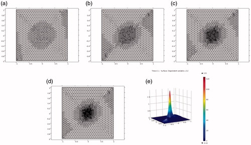
Figure 2. Test 1(b). (a)–(d) Locally adaptively refined meshes of . (e) Computed solution on the four times adaptively refined mesh (d).
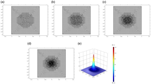
Table 1. Test 1(a). Computed errors and
on the adaptively refined meshes. Here, the solution
is computed using semi-streamline diffusion method of Section 4.1 with
in the adaptive algorithm and
in (86).
Table 2. Test 1(b). Computed errors and
on the adaptively refined meshes. Here, the solution
is computed using semi-streamline diffusion method of Section 4.1 with
in the adaptive algorithm and
in (86).
We present the final solution computed on the four times adaptively refined mesh on the for Test 1(a) and on the for Test 1(b). We note that in both cases we have obtained smoother computed solution
without any oscillatory behavior. This is a significant improvement of the result of Asadzadeh and Larsen (Citation2008) where mainly oscillatory solution could be obtained.
6.2. Test 2
In this test, we perform numerical simulations for the problem (73) with Maxwellian initial condition (87) and for different values of the parameter . Again we use the error indicator (84) in the adaptive algorithm for local refinement of meshes and perform two set of tests as in the case of Test 1 and with the same values on the parameter
.
For finite element discretization we use CSD method as in the Test 1. To be able to control the formation of the layer which appears at the central point we use different values of
inside the function (87). Our computational tests show that the value of the parameter
is optimal.
We present results of our computations for in for Tests 2(a) and 2(b), respectively. Using these tables and and once again, we observe significant reduction of the computational error
on the adaptively refined meshes. Using again, we observe more significant reduction of the computational error in the case (a) than in the case (b). Thus, choosing the parameter
in (84) yields better computational results.
Figure 3. Test 2(a). (a)–(d) Locally adaptively refined meshes of . (e) Computed solution on the four times adaptively refined mesh (d).
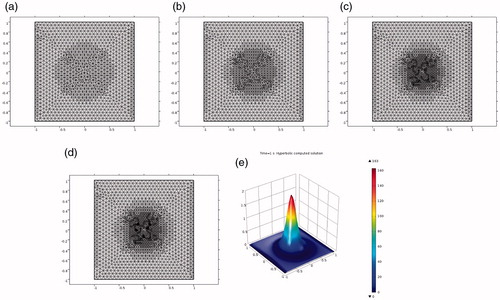
Figure 4. Test 2(b). (a)–(d) Locally adaptively refined meshes of . (e) Computed solution on the four times adaptively refined mesh (d).
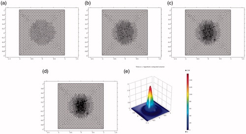
Table 3. Test 2(a). Computed values of errors and
on the adaptively refined meshes. Here, the solution
is computed using characteristic streamline diffusion method with
in the adaptive algorithm.
Table 4. Test 2(b). Computed values of errors and
on the adaptively refined meshes. Here, the solution
is computed using characteristic streamline diffusion method with
in the adaptive algorithm.
Final solution computed on the four times adaptively refined mesh is shown on for Test 2(a) and on for Test 2(b). Again we observe that, with the above numerical values for the parameters, α and
we have avoided the formation of layers and in both tests we have obtained smooth computed solution
.
6.3. Test 3
In this test, we perform numerical simulations of the problem (73) with hyperbolic initial condition (88) on the locally adaptively refined meshes. Taking into account results of our previous Tests 1 and 2 we take fixed value of in (88). For finite element discretization we used the SSD method of Section 4. We again perform two set of tests with different values of
in (84): in Test 3(a) we choose
, and in Test 3(b) we assign this parameter to be
.
We present results of our computations in and . Using these tables and and we observe significant reduction of the computational error on the adaptively refined meshes. Final solutions
computed on the four times adaptively refined meshes are shown on for Test 3(a) and on for Test 3(b), respectively.
Figure 5. Test 3(a). (a)–(d) Locally adaptively refined meshes of . (e) Computed solution on the four times adaptively refined mesh (d).
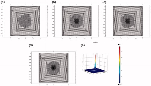
Figure 6. Test 3(b). (a)–(d) Locally adaptively refined meshes of . (e) Computed solution on the four times adaptively refined mesh (d).
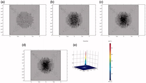
Table 5. Test 3(a). Computed values of errors and
on the adaptively refined meshes. Here, the solution
is computed using semi-streamline diffusion method with
in the adaptive algorithm.
Table 6. Test 3(b). Computed values of errors and
on the adaptively refined meshes. Here, the solution
is computed using semi-streamline diffusion method with
in the adaptive algorithm.
7. Conclusion
In this work, FEM is applied to compute approximate solution of a, degenerate type, convection dominated convection-diffusion problem. We studied different finite element discretizations for the solutions of pencil-beam models based on Fermi and Fokker–Planck equations. The objective was to derive stability estimates and prove optimal convergence rates (due to the maximal available regularity of the exact solution). We specified some “goal-oriented” numerical schemes derived using a variety of Galerkin methods such as standard Galerkin, SSD, characteristic Galerkin, and CSD methods.
Our focus has been in two of these approximation schemes: (i) the SSD and (ii) the CSD methods. The SSD scheme automatically adds extra diffusion to the system, whereas in the CSD the shock capturing property is more pronounced. Both methods are efficient in improving stability and also layer resolution.
For these two settings, we formulated an adaptive algorithm. The Fermi equation, with the initial data of the form (however with constant σtr) has a closed-form analytic solution. This analytic solution is used as an “adequate approximation” to the analytic solutions of our test problems. This is due to the following facts that we have proved stability of the considered schemes and in our numerical tests the initial data are approximating
, the initial data for the Fermi equation. Also the closed-form solution is used to make local mesh refinements.
Numerically, we tested our adaptive algorithm for different types of initial data in (73) in three tests with different mesh refinement parameters in the mesh refinement criterion (84). The initial data in the tests, although all approximating the product of Dirac functions, are chosen with different kind of singularities.
The goal of our numerical experiments was to remove oscillatory behavior of the computed solution in Asadzadeh and Larsen (Citation2008) as well as removing of the formation of the artificial and boundary layers that appeared, for example, in Naqos (Citation2005).
Based on the results of this study, we conclude that the SD approach decreases the dominance of the convection. Further the, local refinement based-adaptivity strategy can remove both the oscillatory behavior of the computed solutions and layer formations appearing for problems with nonsmooth initial data.
Additional information
Funding
References
- Adams, A. R. 1975. Sobolev spaces. New York, NY: Academic Press.
- Asadzadeh, M., and A. Sopasakis. 2002. On fully discrete schemes for the Fermi pencil-beam equation. Comput. Methods Appl. Mech. Eng. 191 (1):4641–4659.
- Asadzadeh, M., and E. Larsen. 2008. Linear transport equations in flatland with small angular diffusion and their finite element approximation. Math. Comput. Model (Elsevier). 47:495–514.
- Asadzadeh, M. 1997. Streamline diffusion methods for Fermi and Fokker-Planck equations. Transport Theory Stat. Phys. 26 (3):319–340.
- Asadzadeh, M. 2000. A posteriori error estimates for the Fokker-Planck and Fermi pencil beam equations. Math. Models Meth. Appl. Sci. 48,10 (5):737–769.
- Asadzadeh, M. 2002. On the stability of characteristic schemes for the Fermi equation. Appl. Comput. Math. 1(1):158–174.
- Borgers, C., and E. W. Larsen. 1996. Asymptotic derivation of the Fermi pencil-beam approximation. Nucl. Sci. Eng. 123:343–357.
- Brenner, S. C., and L. R. Scott. 1994. The mathematical theory of finite element methods. Berlin: Springer-Verlag.
- Ciarlet, P. G. 1941 [1980]. The finite element method for elliptic problems. New York, Oxford: Amsterdam North-Holland.
- Eyges, L. 1948. Multiple scattering with energy loss. Phys. Rev. 74:1534–35.
- Johnson, C. 1992. A new approach to algorithms for convection problems which are based on exact transport + projection. Comput. Methods Appl. Mech. Eng. 100:45–62.
- Larsen, E. W., C. D. Levermore, G. C. Pomraning, and J. G. Sanderson. 1985. Discretization methods for one-dimensional Fokker-Planck operators. J. Comput. Phys. 61 (3):359–390.
- Luo, Z.-M. and A. Brahme. 1993. An overview of the transport theory of charged particles. Radiat. Phys. Chem. 41:673.
- Naqos, S. 2005. Numerical algorithms for electron beams. Master thesis, Chalmers University of Technology, Department of Mathematics.
- Pomraning, G. C. 1992. The Fokker-Planck operator as an asymptotic limit. Math. Models Meth. Ap. Sci. 2:21.
- Prinja, A. K., and G. C. Pomraning. 1996. One-dimensional beam transport. Transp. Theory Statist. Phys. 25 (2):231–247.
- Rossi, B., and K. Greisen. 1941. Cosmic-ray theory. Rev. Mod. Phys. 13:265.