Convergence of hp-Streamline Diffusion Method for Vlasov–Maxwell System

Abstract

In this paper we study stability and convergence for hp-streamline diffusion (SD) finite element method for the, relativistic, time-dependent Vlasov–Maxwell (VM) system. We consider spatial domain ${\Omega }_x\subset {\mathbf{R}}^3$ and velocities $\mathbf{v}\in {\Omega }_v\subset {\mathbf{R}}^3.$ The objective is to show globally optimal a priori error bound of order $\mathcal{O}{(h/p)}^{s+1/2},$ for the SD approximation of the VM system; where $h (={\max }_K{h}_K)$ is the mesh size and $p (={\max }_K{p}_K)$ is the spectral order. Our estimates rely on the local version with h_K being the diameter of the phase-space-time element K and p_K the spectral order for K. The optimal hp estimates require an exact solution in the Sobolev space $H^{s+1}(\Omega ).$ Numerical implementations, performed for examples in one space- and two velocity dimensions, are justifying the robustness of the theoretical results.

Keywords:

• Vlasov–Maxwell
• stability
• convergence
• hp method

1. Introduction

In the SD method the weak form is modified by adding a multiple of the streaming part in the equation, to the test function. So we obtain a multiple of streaming terms in both test and trial functions. This can be viewed as an extra diffusion in the streaming direction in the original equation. Hence, the name of the method (the streamline diffusion). Such an extra diffusion would improve both the stability and convergence properties of the underlying Galerkin scheme. It is well known that the standard Galerkin method, used for hyperbolic problems, has a suboptimal behavior: Converges as $\mathcal{O}(h^{s-1})$ (versus $\mathcal{O}(h^s)$ for the elliptic and parabolic problems with exact solution in the same space: $H^s(\Omega )$). The SD method improves this drawback by $\mathcal{O}(h^{1/2}),$ also, having an upwinding character, enhances the stability. The properties that are achieved by the discontinuous Galerkin as well. The hp-approach is to capture local behavior in the sense that: in the vicinity of singularities refined mesh h is combined with the lower spectral order (small p), whereas in more smooth regions higher order polynomials (large p) and non-refined (large h) meshes are used. Hence, the hp-approach may be viewed as a kind of automatic adaptivity.

The Vlasov–Maxwell (VM) system describing the time evolution of collisionless plasma is formulated as (1.1) $$\begin{array}{c}{\partial }_{t}f+\widehat{v}·{\nabla }_{x}f+q(E+c^{-1}\widehat{v}\times B)·{\nabla }_{v}f=0,\\ {\partial }_{t}E=c{\nabla }_x\times B-j,\hspace{1em}{\nabla }_x·E=\rho ,\\ {\partial }_{t}B=-c{\nabla }_x\times E,\hspace{1em}{\nabla }_x·B=0\end{array}$$(1.1) with, physically relevant, initial data $f(0,x,v)=f^0(x,v)\ge 0,E(0,x)=E^0(x),B(0,x)=B^0(x).$ Here f is the density, in phase space, time of particles with charge q, mass m and velocity $$\widehat{v}={(m^2+c^{-2}|v{|}^2)}^{-1/2}v\hspace{1em}(v \text{is} \text{momentum}).$$

Moreover, c is the speed of light and the charge and current densities: ρ and j are (1.2) $$\rho (t,x)=4\pi \int qf dv\hspace{1em}\text{and}\hspace{1em}j(t,x)=4\pi \int qf\widehat{v} dv.$$(1.2)

The Vlasov–Maxwell equations arise in several context such as, e.g., continuum, plasma physics and rarefied gas dynamics, where the main assumption underlying the model is that collisions are rare and therefore negligible. The system (1.1)(1.1) $$\begin{array}{c}{\partial }_{t}f+\widehat{v}·{\nabla }_{x}f+q(E+c^{-1}\widehat{v}\times B)·{\nabla }_{v}f=0,\\ {\partial }_{t}E=c{\nabla }_x\times B-j,\hspace{1em}{\nabla }_x·E=\rho ,\\ {\partial }_{t}B=-c{\nabla }_x\times E,\hspace{1em}{\nabla }_x·B=0\end{array}$$(1.1) is modeling the motion of a collisionless plasma, e.g., a high-temperature, low-density, ionized gas. The mathematical challenge in study of the Vlasov–Maxwell system is the presence of the nonlinear term: $(E+\widehat{v}\times B)·{\nabla }_{v}f.$ In the case of divergence free field, this term is written as ${\text{div}}_v\left(\right(E+\widehat{v}\times B\left)f\right).$ A thorough mathematical analysis, with such nonlinearity, is studied by Di Perna and Lions in DiPerna and Lions (1989).

An outline of the remaining part of this paper is as follows: In Section 2 we present the canonical form of the equations and state the numerical approximation strategy. Section 3 describes hp and SD strategies. Section 4 is devoted to the approximation of the projection error. In Section 5 we study the convergence of the constructed schemes. In our concluding Section 6 we implement some numerical examples in a lower dimensional case that justifies our theoretical study.

2. Canonical forms

As a general framework we introduce similar convective forms f or both Vlasov and Maxwell equations. The convection coefficients are nonlinear vector functions for the Vlasov equation and constant sparse multiple matrices in the Maxwell case. Despite physical diversities, these coefficients are exhibiting a common property: they both are divergence free, a property that substantially simplifies the analysis. Let $E={(E_1,E_2,E_3)}^T,B={(B_1,B_2,B_3)}^T,j={(j_1,j_2,j_3)}^T,$ then the Maxwell’s equations can be written as $$\{\begin{array}{c}{\partial }_t{E}_1={\partial }_2{B}_3-{\partial }_3{B}_2-j_1,\hfill \\ {\partial }_t{E}_2={\partial }_3{B}_1-{\partial }_1{B}_3-j_2,\hfill \\ {\partial }_t{E}_3={\partial }_1{B}_2-{\partial }_2{B}_1-j_3,\hfill \end{array}\hspace{1em}\text{and}\hspace{1em}\{\begin{array}{c}{\partial }_t{B}_1=-{\partial }_2{E}_3+{\partial }_3{E}_2,\hfill \\ {\partial }_t{B}_2=-{\partial }_3{E}_1+{\partial }_1{E}_3,\hfill \\ {\partial }_t{B}_3=-{\partial }_1{E}_2+{\partial }_2{E}_1,\hfill \end{array}$$ where ${\partial }_i$ denotes the derivative with respect to x_i. We also introduce 6 × 6 symmetric matrices $M_k, k=1,2,3$: (2.1) $$\{\begin{array}{ccc}{\left(M_1\right)}_{35}={\left(M_1\right)}_{53}=-1,\hfill & \hfill & \text{else}\hspace{1em}{\left(M_1\right)}_{ij}={\left(M_1\right)}_{ji}=0,\hfill \\ {\left(M_2\right)}_{16}={\left(M_2\right)}_{61}=-1,\hfill & {\left(M_2\right)}_{34}={\left(M_2\right)}_{43}=1,\hfill & \text{else}\hspace{1em}{\left(M_2\right)}_{ij}={\left(M_2\right)}_{ji}=0,\hfill \\ {\left(M_3\right)}_{24}={\left(M_3\right)}_{42}=-1,\hfill & {\left(M_3\right)}_{15}={\left(M_3\right)}_{51}=1,\hfill & \text{else}\hspace{1em}{\left(M_3\right)}_{ij}={\left(M_3\right)}_{ji}=0.\hfill \end{array}$$(2.1)

To write the Maxwell equations in the matrix-vector form, we introduce the matrix-vector notation $\mathbf{M}=(M_1,M_2,M_3),$ and set $\mathbf{E}=(E_1,E_2,E_3),$ $\mathbf{B}=(B_1,B_2,B_3),\mathbf{j}=(j_1,j_2,j_3),\mathbf{0}=(0,0,0),\mathbf{b}=(\mathbf{j},\mathbf{0}).$ Further let $\mathbf{W}={(\mathbf{E},\mathbf{B})}^T$ and use the notations for the initial values ${\mathbf{E}}^{\mathbf{0}},{\mathbf{B}}^{\mathbf{0}},{\mathbf{W}}^{\mathbf{0}}.$ Then (2.2) $$\{\begin{array}{c}{\partial }_t\mathbf{W}+\mathbf{M}·\nabla \mathbf{W}=\mathbf{b},\hfill \\ \mathbf{W}(0,x)={\mathbf{W}}^0\left(x\right).\hfill \end{array}$$(2.2)

Note that (2.2)(2.2) $$\{\begin{array}{c}{\partial }_t\mathbf{W}+\mathbf{M}·\nabla \mathbf{W}=\mathbf{b},\hfill \\ \mathbf{W}(0,x)={\mathbf{W}}^0\left(x\right).\hfill \end{array}$$(2.2) is convective with, matrix-vector form, divergent free ($\mathbf{DivM}=\mathbf{0}$) convection coefficient.

The Vlasov possesses a similar structure, but with nonlinear coefficient vectors depending on x and v: (2.3) $$\{\begin{array}{c}{\partial }_{t}f+\widehat{v}·{\nabla }_{x}f+(E+\widehat{v}\times B)·{\nabla }_{v}f=0,\hfill \\ f(0,x,v)=f^0(x,v)\ge 0,\hfill \end{array}$$(2.3) which can be rewritten in a compact form as (2.4) $${\partial }_{t}f+G\left(f\right)·\nabla f=0.$$(2.4) where $\nabla f=({\nabla }_{x}f,{\nabla }_{v}f)$ is the total gradient and $G\left(f\right)=(\widehat{v},E+\widehat{v}\times B)$ is divergence free: (2.5) $$\text{div} G\left(f\right)=\sum _{i=1}^d\frac{\partial \widehat{v}}{\partial x_i}+\sum _{i=d+1}^{2d}\frac{\partial (E+\widehat{v}\times B)}{\partial v_{i-d}}={\nabla }_v(\widehat{v}\times B)=0.$$(2.5)

Throughout the paper C will denote a generic constant, not necessarily the same at each occurrence, unless otherwise explicitly specified.

2.1. The numerical approximation strategy

Consider a function F in an infinite dimensional Hilbert (or Banach) space $\mathcal{F}.$ We want to approximate F with a function $\tilde{F}$ in a finite dimensional subspace $\tilde{\mathcal{F}}$ of $\mathcal{F}.$ To this end, first we assume a classical form approximation (an interpolant, or a projection, e.g. L₂- or Ritz-projection) $\Pi F\in \tilde{\mathcal{F}}$ of F. Then, roughly, the idea is i) to use (or establish) a theoretical error estimate, in a certain norm, for the interpolation or projection error $F-\Pi F,$ and ii) split the numerical error as $$F-\tilde{F}=(F-\Pi F)+(\Pi F-\tilde{F}):=\eta +\xi ,$$ and prove that there is a constant C such that (2.6) $$\left|\right|\xi \left|\right|\le C\left|\right|\eta \left|\right|.$$(2.6)

The intermediate (theoretical) part, i.e., control of $\left|\right|\eta \left|\right|,$ is the most crucial step in the efficiency of the numerical approximation procedure. The numerical approach gets its reliability from the stability of the constructed numerical method and its accuracy from the convergence analysis.

3. The SD and hp structures

3.1. Constructing finite element spaces

For numerical studies we need to restrict the variables to bounded domains: ${\Omega }_x\subset {\mathbf{R}}^3$ and ${\Omega }_v\subset {\mathbf{R}}^3,$ as the space and velocity, respectively. We assume that $f(t,x,v),E_i(t,x)$ and $B_i(t,x),$ for i = 1, 2, 3, have compact supports in Ω_x and that $f(t,x,v)$ has compact support in both Ω_x and Ω_v. Assume that $h (0<h<1),$ and let $T_h^x=\left\{{\tau }_x\right\}$ and $T_h^v=\left\{{\tau }_v\right\}$ be finite element subdivisions of Ω_x with elements τ_x and Ω_v with elements τ_v, respectively. Then $T_h=T_h^x\times T_h^v=\{{\tau }_x\times {\tau }_v\}=\left\{\tau \right\}$ is a subdivision of Ω. (with a, phase-space, mesh size h). Let now $0=t_0<t_1<\dots <t_{N-1}<t_N=T$ be a partition of the time interval $[0,T]$ into sub-intervals $I_n=(t_{n-1},t_n],$ with $\left|I_n\right|:=t_n-t_{n-1}=:k_n\approx h,n=1,\dots ,N.$ Further let ${\mathcal{C}}_h$ be the corresponding subdivision of $Q_T=[0,T]\times \Omega$ into the prismatic elements $K=I_n\times \tau ,$ with $h_K=\text{diam} K$ as the mesh parameter. We also define a piecewise constant mesh function $h(t,x,v):=h_K,(t,x,v)\in K.$ Finally, induced from ${\mathcal{C}}_h,$ we introduce ${\tilde{\mathcal{C}}}_h$ as the finite element subdivision of $[0,T]\times {\Omega }_x.$

Remark 3.1.

From now on, the discrete schemes are the finite element approximations of Equations (2.2)(2.2) $$\{\begin{array}{c}{\partial }_t\mathbf{W}+\mathbf{M}·\nabla \mathbf{W}=\mathbf{b},\hfill \\ \mathbf{W}(0,x)={\mathbf{W}}^0\left(x\right).\hfill \end{array}$$(2.2) and (2.3)(2.3) $$\{\begin{array}{c}{\partial }_{t}f+\widehat{v}·{\nabla }_{x}f+(E+\widehat{v}\times B)·{\nabla }_{v}f=0,\hfill \\ f(0,x,v)=f^0(x,v)\ge 0,\hfill \end{array}$$(2.3) with $(x,v,t)\in (0,T]\times {\Omega }_x\times {\Omega }_v,$ associated with initial and boundary conditions. Assuming also that f has compact support in the velocity space we get homogeneous Dirichlet boundary condition for Ω_v.

To formulate variational (weak) form of the VM system we introduce the product spaces $${\mathcal{H}}_0=\prod _{n=1}^N{\mathcal{H}}_0^1\left({\Omega }_n\right)\hspace{1em}\text{and}\hspace{1em}{\tilde{\mathcal{H}}}_0=\prod _{n=1}^N{\mathcal{H}}_0^1\left({\tilde{\Omega }}_n\right),$$ where ${\Omega }_n:=I_n\times {\Omega }_x\times {\Omega }_v,$ ${\tilde{\Omega }}_n:=I_n\times {\Omega }_x,$ and for $\Omega :={\Omega }_x\times {\Omega }_v$$${\mathcal{H}}_0^1(I_n\times \Omega ):=\{w\in H^1(I_n\times \Omega );w=0 \text{on} \partial \Omega \}.$$

For $k=0,1,2,\dots ,$ we define the finite element spaces for the Maxwell’s equations (resp. Vlasov equation) as being the space of piecewise polynomials that are continuous in x (resp. in x and v) with possible discontinuities at the interior time levels $t_n, n=1,\dots ,N-1$: $${\tilde{V}}_h=\{g\in {\left[{\tilde{\mathcal{H}}}_0\right]}^6;g_i{|}_{\tilde{K}}\in P_{p_{\tilde{K}}}(I_n)\times P_{p_{\tilde{K}}}({\tau }_x), \forall \tilde{K}=I_n\times {\tau }_x\in {\tilde{\mathcal{C}}}_h, 1\le i\le 6\},$$ with the extension for the Vlasov part and with $\tau ={\tau }_x\times {\tau }_v$ as $$V_h=\{g\in {\mathcal{H}}_0;g{|}_K\in P_{p_K}(I_n)\times P_{p_K}({\tau }_x)\times P_{p_K}({\tau }_v), \forall K=I_n\times \tau \in {\mathcal{C}}_h\}.$$ where $P_{p_K}(·)$ is the set of polynomial of degree at most p_K on the underlying set. Here we allow the degree of polynomial to vary from elementwise. Therefore we may define the piecewise constant function $p(t,x,v):=p_K.$ Finally we shall use the following notation: $$\begin{array}{c}{(f,g)}_n={(f,g)}_{S_n},\hspace{1em}\Vert g{\Vert }_n={(g,g)}_n^{1/2}\\ {〈f,g〉}_n={\left(f\right(t_n,\dots ),g(t_n,\dots \left)\right)}_{\Omega },\hspace{1em}|g{|}_n={〈g,g〉}_n^{1/2},\end{array}$$ where, for $n=1,\dots ,N,S_n:={\tilde{\Omega }}_n,$ for the Maxwell’s equations and $S_n:={\Omega }_n$ in the Vlasov case.

3.2. The SD strategy

The idea of the weak form for a differential equation, e.g., variational formulation and the finite element methods, rely on the basic structure of the Fourier transformation: to multiply the function f by a basis function $e^{-ix\xi }$ and integrate. Then for each $\xi \in \mathbf{R}$ we extract an information, $\widehat{f}\left(\xi \right),$ from the function f (these are the Fourier coefficients when considering Fourier series). In this way we get an “excessive amount ($\infty$) of information,” which (i) is unrealistic to tackle and (ii) contains a great deal of unnecessary data. The remedy is a clever choice of a finite number of, treatable, multipliers that provides the most crucial information needed. This is basically the goal of the Galerkin approach with finitely many multipliers. However, here we need to extract the information from the PDE itself rather than its solution. We seek an approximate solution for a PDE in a finite dimensional space (trial space) with the multipliers being in the same or a closely related finite dimensional space known as the test function space. The idea with the SD method is to multiply the underlying PDE by a sum of the test function and a multiple of an expression as the streaming term in the PDE, with the solution is replaced by the test function, say g. Hence, we consider a common form for (2.2)(2.2) $$\{\begin{array}{c}{\partial }_t\mathbf{W}+\mathbf{M}·\nabla \mathbf{W}=\mathbf{b},\hfill \\ \mathbf{W}(0,x)={\mathbf{W}}^0\left(x\right).\hfill \end{array}$$(2.2) and (2.4)(2.4) $${\partial }_{t}f+G\left(f\right)·\nabla f=0.$$(2.4) , viz. (3.1) $$F_t+\mu ·\nabla F=b,$$(3.1) and formulate the SD scheme to find the solution F such that (3.2) $$(F_t+\mu ·\nabla F,g+\delta \mu ·\nabla g)=(b,g+\delta \mu ·\nabla g).$$(3.2)

Expanding Equation (3.2)(3.2) $$(F_t+\mu ·\nabla F,g+\delta \mu ·\nabla g)=(b,g+\delta \mu ·\nabla g).$$(3.2) we get a term of the form $\delta (\mu ·\nabla F,\mu ·\nabla g).$ Setting g = F, this term can be interpreted as coming from a diffusion term $-\delta {\Delta }_{\mu }F,$ of order δ, in the streamline direction μ, hence the name of the method.

3.3. The hp approach

Here, we introduce the main function spaces employed in hp-studies for approximating the projection errors, (see, e.g. Houston et al. 2000): Let $\mathcal{P}$ be a partition of ${\Omega }_T=(0,T)\times {\Omega }_x\times {\Omega }_v$ into open patches P which are images of canonical “cubes”: $\widehat{P}={(-1,1)}^{2d+1}:={\left(\widehat{I}\right)}^{2d+1}, d=1,2,3,$ under smooth bijections F_P: $$\forall P\in \mathcal{P}:\hspace{1em}P=F_P\left(\widehat{P}\right).$$

We construct a mesh $\mathcal{T}:={\cup }_{P\in \mathcal{P}}{\mathcal{T}}_P$ on Ω_T by subdividing each $\widehat{P}={(-1,1)}^{2d+1},$ into $2d+1$-dimensional generalized quadrilateral elements $\widehat{\tau },$ or $2d+1$-dimensional prisms. We label them as $\widehat{\tau }$ which are affine equivalent to $\widehat{P},$ and call the mesh ${\widehat{\mathcal{T}}}_P$ (on $\widehat{P}$). Then, on each $P\in \mathcal{P}$ we define a mesh ${\mathcal{T}}_P$ by setting $$\forall P\in \mathcal{P}:\hspace{1em}{\mathcal{T}}_P:=\left\{\tau \right|\tau =F_P\left(\widehat{\tau }\right), \widehat{\tau }\in {\widehat{\mathcal{T}}}_P\}.$$

Each $\widehat{\tau }\left(\tau \right)$ is an image of the domain $\widehat{P}$ under an affine mapping $A_{\widehat{\tau }}:\widehat{P}\to \widehat{\tau }(F_{\tau }=F_P°A_{\widehat{\tau }}:\widehat{P}\to \tau ).$ Next we define the space $$F_{\mathcal{P}}=\{F_P:P\in \mathcal{P}\},$$ and the polynomial space $${\mathcal{A}}_p=\text{span}\{{(\widehat{x},\widehat{v},\widehat{t})}^{\alpha }:0\le {\alpha }_i\le p, 1\le i\le 2d+1\},$$ where $(\widehat{x},\widehat{v},\widehat{t})\in \widehat{P}:=\left\{\right(\widehat{x},\widehat{v},\widehat{t})\in {\mathbf{R}}^d\times {\mathbf{R}}^d\times {\mathbf{R}}^{+}:|{\widehat{x}}_j|\le 1 \& |{\widehat{v}}_j|\le 1, \widehat{t}\le 1\hspace{1em}j=1,\dots ,d\},$ and $\alpha =({\alpha }_1,{\alpha }_2,\dots ,{\alpha }_{2d+1})$ is multi-index Moreover let p be a polynomial degree vector in $\mathcal{T},$$$\mathbf{p}=\{p_{\tau }:\tau \in \mathcal{T}\},$$ and define the continuous hp-finite element spaces $$S^{\mathbf{p},k}({\Omega }_T,\mathcal{T},F_{\mathcal{P}}):=\{f\in H^k({\Omega }_T):f{|}_{\tau }°F_{\tau }\in {\mathcal{A}}_{p_{\tau }},\hspace{1em}\tau \in \mathcal{T}\},\hspace{1em}k=0,1,\dots ,$$ for polynomials with degree vector p, and with $$S^{p,k}({\Omega }_T,\mathcal{T},F_{\mathcal{P}}):=\{f\in S^{\mathbf{p},k}({\Omega }_T,\mathcal{T},F_{\mathcal{P}}):\mathbf{p}=(p,p,\dots ,p\left)\right\},$$ for the uniform polynomial degree $p_{\tau }=p, \forall \tau , p>1.$ Finally we denote by $\left|\right|f|{|}_{k,\widehat{I}}$ and $|f{|}_{k,\widehat{I}}$ the $H^k\left(\widehat{I}\right)$ norm and seminorm on $\widehat{I},$ respectively (we shall suppress k = 0, corresponding to the L₂-norm). We also denote by $S^p\left(\widehat{I}\right)$ the set of polynomials of degree p on $\widehat{I}.$ In the Maxwell case one needs to replace the domain ${\Omega }_T={\Omega }_x\times {\Omega }_v\times (0,T)$ by ${\tilde{\Omega }}_T={\Omega }_x\times (0,T).$

4. Approximation of the projection error

The projection error estimates are of analytic nature and often predictable, however too involved to derive. In this section we provide estimates, without proofs, for $\left|\right|\eta \left|\right|$ and $\left|\right|\mathcal{D}\eta \left|\right|,$ where $\mathcal{D}:=({\nabla }_x,{\nabla }_v,d/dt)$ denotes the total gradient operator. We denote by ${\pi }_p^{i}f$ the 1-dimensional H¹-projection of f onto the polynomials of degree p in the ith coordinate, where $1\le i\le d$ would correspond to x_i’s for the spatial variable, $d+1\le i\le 2d$ to v_i’s for the velocity, and $i=2d+1$ for the time variable. We shall apply the tensor product in $2d+1$-dimensions to the following one-dimensional results by Schwab (1998).

Proposition 4.1.

Let $f\in H^{k+1}\left(\widehat{I}\right), \widehat{I}=(-1,1)$ for some $k\ge 0$. Then, for every $p\ge 1$, there exists a projection ${\pi }_{p}f\in S^p\left(\widehat{I}\right)$ such that, for any $0\le s\le \min (p,k),$(4.1) $$\Vert f^{\prime }-{\left({\pi }_{p}f\right)}^{\prime }{\Vert }_{\widehat{I}}^2\le \frac{(p-s)!}{(p+s)!}|f{|}_{s+1,\widehat{I}}^2,$$(4.1) (4.2) $$\Vert f-{\pi }_{p}f{\Vert }_{\widehat{I}}^2\le \frac{1}{p(p+1)}\frac{(p-s)!}{(p+s)!}|f{|}_{s+1,\widehat{I}}^2.$$(4.2)

The theorem below is a generalized version of Proposition 4.1, in $2d+1$ dimensions with ${\Pi }_p={\prod }_{i=1}^{2d+1}{\pi }_p^i$: the tensor product projectors and binary multi-index $|m{|}_l\equiv {\sum }_{n=1}^l{m}_n,$ with m_n = 0 or 1, is derived in Asadzadeh and Sopasakis (2007).

Theorem 4.2.

Let ${\mathcal{T}}_h=\cup K$ be a partition of the domain $D\subset {\mathbf{R}}^{\mathcal{N}},$ and $K\in {\mathcal{T}}_h$ be an image of the $\mathcal{N}$-dimensional canonical hypercube $\widehat{R}:={(-1,1)}^{\mathcal{N}}$, with $\mathcal{N}$-dimensional mesh ${\mathcal{T}}_{\widehat{R}}$, under the bijection $G_K: \tau =G_K\left(\widehat{R}\right)$. For the polynomial degree distribution $\mathbf{r}=\{r_K | K\in {\mathcal{T}}_h\}$ and $\forall K\in {\mathcal{T}}_h$, let $f{|}_K\in H^{k_K+1}\left(K\right)$ for some $k_K\ge 1$. Then, for $r_K\ge 1$ and $0\le s_K\le \min (r_K,k_K)$ we have$$\begin{array}{c}\left|\right|\eta |{|}^2\le C\sum _{K\in {\mathcal{T}}_h}{\left(\frac{h_K}{2}\right)}^{2s_K+2}{\Phi }_1(r_K,s_K\left)\right|\left|\widehat{f}\right|{|}_{s_K+1,\widehat{K}}^2,\\ \left|\right|\mathcal{D}\eta |{|}^2\le C\sum _{K\in {\mathcal{T}}_h}{\left(\frac{h_K}{2}\right)}^{2s_K}{\Phi }_2(r_K,s_K\left)\right|\left|\widehat{f}\right|{|}_{s_K+1,\widehat{K}}^2,\end{array}$$with $\widehat{f}=f°G_{\tau },K=G_{\tau }\left(\widehat{K}\right), \left|\right|·|{|}_{s_K+1,\widehat{K}}$ is the Sobolev norm in $H^{s_K+1}\left(\widehat{K}\right)$ and$$\begin{array}{c}{\Phi }_1(p,s)=\mathcal{N}\sum _{i=1}^{\mathcal{N}}{2}^{i-1}\sum _{|m{|}_{i-1}\le i-1}{\alpha }_p^{|m{|}_{i-1}+1}{\beta }_{|m{|}_{i-1}},\\ {\Phi }_2(p,s)=\mathcal{N}\sum _{i=1}^{\mathcal{N}}\sum _{j=1}^{\mathcal{N}}{2}^j\sum _{\underset{m_i=1}{|m{|}_{j-1}\le j-1}}{\alpha }_p^{|m{|}_{j-1}}{\beta }_{|m{|}_{j-1}}.\end{array}$$ where ${\partial }^{|m{|}_{i-1}}={\partial }_1^{m_1}{\partial }_2^{m_2}\cdots {\partial }_{i-1}^{m_{i-1}}, {\alpha }_p=\frac{1}{p(p+1)},$ and ${\beta }_{|m{|}_k}=\frac{(p-s+|m{|}_k)!}{(p+s-|m{|}_k)!}.$

The proof is based on a scaling argument for an affine mapping and a generalization of the Proposition 4.1.

Remark 4.3.

The above estimates relying on Sobolev inequalities are dimension dependent and give rise to singularities in higher dimensions. In addition, the bound for s ($0\le s\le \min (p,k)$) and the fact that the spectral order p cannot be chosen very large, limits the value of $|m{|}_k$ in ${\beta }_{|m{|}_k}$ to $|m{|}_k<p+s.$ This yields additional bounds for the indices of the interior sums.

Using Stirling’s formula, see Houston et al. (2000), one can show that $$\max \left({\Phi }_2\right(p,s),{\Phi }_2(p,s\left)\right)\le C{p}^{-2s}.$$

An estimate that is crucial in deriving p-version of hp estimates.

5. Convergence analysis

Due to the common structure for the Maxwell (2.2)(2.2) $$\{\begin{array}{c}{\partial }_t\mathbf{W}+\mathbf{M}·\nabla \mathbf{W}=\mathbf{b},\hfill \\ \mathbf{W}(0,x)={\mathbf{W}}^0\left(x\right).\hfill \end{array}$$(2.2) and Vlasov (2.4)(2.4) $${\partial }_{t}f+G\left(f\right)·\nabla f=0.$$(2.4) equations, and since the hp-SD approach has been considered for (2.4)(2.4) $${\partial }_{t}f+G\left(f\right)·\nabla f=0.$$(2.4) in Asadzadeh and Sopasakis (2007), below we give the details only in the Maxwell case (2.2)(2.2) $$\{\begin{array}{c}{\partial }_t\mathbf{W}+\mathbf{M}·\nabla \mathbf{W}=\mathbf{b},\hfill \\ \mathbf{W}(0,x)={\mathbf{W}}^0\left(x\right).\hfill \end{array}$$(2.2) .

5.1. hp-method for Maxwell equations

Starting with, sufficiently smooth, f⁰, b⁰ and W⁰, let $f^{h,i},b^{h,i}$ and $W^{h,i}$ denote the approximations on the ith iteration step (i > 0) for f, b and W, respectively. The h version of the SD method on the ith step for the Maxwell’s part (with the short operator notation: $M·\nabla :={\sum }_{\ell =1}^3{M}_{\ell }{\partial }_{\ell },$ recall that $M_{\ell }$ are the 6 × 6 matrices in (2.1)(2.1) $$\{\begin{array}{ccc}{\left(M_1\right)}_{35}={\left(M_1\right)}_{53}=-1,\hfill & \hfill & \text{else}\hspace{1em}{\left(M_1\right)}_{ij}={\left(M_1\right)}_{ji}=0,\hfill \\ {\left(M_2\right)}_{16}={\left(M_2\right)}_{61}=-1,\hfill & {\left(M_2\right)}_{34}={\left(M_2\right)}_{43}=1,\hfill & \text{else}\hspace{1em}{\left(M_2\right)}_{ij}={\left(M_2\right)}_{ji}=0,\hfill \\ {\left(M_3\right)}_{24}={\left(M_3\right)}_{42}=-1,\hfill & {\left(M_3\right)}_{15}={\left(M_3\right)}_{51}=1,\hfill & \text{else}\hspace{1em}{\left(M_3\right)}_{ij}={\left(M_3\right)}_{ji}=0.\hfill \end{array}$$(2.1) ) can be formulated as: find $W^{h,i}\in {\tilde{V}}_h$ such that (5.1) $$\tilde{\mathcal{B}}(W^{h,i},g)=\tilde{\mathcal{L}}(b^{h,i-1};g)\hspace{1em}\forall g\in {\tilde{V}}_h,$$(5.1) where $g={(g_1,\dots ,g_6)}^T,$ with the bilinear form $\tilde{\mathcal{B}}$ defined as $$\tilde{\mathcal{B}}(W,g)=\sum _{n=0}^{N-1}({\partial }_{t}W+M·\nabla W,g+\delta ({\partial }_{t}g+M·\nabla g){)}_n+\sum _{n=1}^{N-1}{〈\left[W\right],g_{+}〉}_m+{〈W_{+},g_{+}〉}_0.$$

$[W]=W_{+}-W_{-}$ denotes the jump ($g_{\pm }(t,x)=\underset{s\to 0^{\pm }}{\lim }g(t+s,x)$), and the linear form $\tilde{\mathcal{L}}$ is given by $$\tilde{\mathcal{L}}(b;g)=\sum _{n=0}^{N-1}(b,g+\delta ({\partial }_{t}g+M·\nabla g){)}_n+{〈W^0,g_{+}〉}_0.$$

Let now ${(·,·)}_K$ denote the L₂ product over K and define a nonnegative piecewise constant function δ by $$\delta {|}_K={\delta }_K,\hspace{1em}\text{for} K\in {\tilde{\mathcal{C}}}_h.$$

We may formulate a finite element method based on the local space-time elements. Then, the problem (5.1)(5.1) $$\tilde{\mathcal{B}}(W^{h,i},g)=\tilde{\mathcal{L}}(b^{h,i-1};g)\hspace{1em}\forall g\in {\tilde{V}}_h,$$(5.1) would have an alternative formulation replacing in the definitions for $\tilde{\mathcal{B}}$ and $\tilde{\mathcal{L}}$ the sum of the inner products ${(·,·)}_n$ involving δ_K by the corresponding sum $\sum _{K\in {\tilde{\mathcal{C}}}_h}{(·,·)}_K$ and all δ by δ_K. Then, (5.1)(5.1) $$\tilde{\mathcal{B}}(W^{h,i},g)=\tilde{\mathcal{L}}(b^{h,i-1};g)\hspace{1em}\forall g\in {\tilde{V}}_h,$$(5.1) will be rewritten as (5.2) $$\tilde{\mathcal{B}}(W,g)=\sum _{K\in {\tilde{\mathcal{C}}}_h}{({\partial }_{t}W+M·\nabla W,g+{\delta }_K({\partial }_{t}g+M·\nabla g\left)\right)}_K+\sum _{n=1}^{N-1}{〈\left[W\right],g_{+}〉}_n+{〈W_{+},g_{+}〉}_0,$$(5.2) and the solution W of Equation (2.2)(2.2) $$\{\begin{array}{c}{\partial }_t\mathbf{W}+\mathbf{M}·\nabla \mathbf{W}=\mathbf{b},\hfill \\ \mathbf{W}(0,x)={\mathbf{W}}^0\left(x\right).\hfill \end{array}$$(2.2) satisfies the variational formulation (5.3) $$\tilde{\mathcal{B}}(W,g)=\tilde{\mathcal{L}}(b;g)\hspace{1em}\forall g\in {\tilde{V}}_h.$$(5.3)

Subtracting Equation (5.1)(5.1) $$\tilde{\mathcal{B}}(W^{h,i},g)=\tilde{\mathcal{L}}(b^{h,i-1};g)\hspace{1em}\forall g\in {\tilde{V}}_h,$$(5.1) from Equation (5.3)(5.3) $$\tilde{\mathcal{B}}(W,g)=\tilde{\mathcal{L}}(b;g)\hspace{1em}\forall g\in {\tilde{V}}_h.$$(5.3) we end up with the following relation: (5.4) $$\tilde{\mathcal{B}}(W-W^{h,i},g)=\tilde{\mathcal{L}}(b;g)-\tilde{\mathcal{L}}(b^{h,i-1};g)\hspace{1em}\forall g\in {\tilde{V}}_h.$$(5.4)

Finally, with jumps at the time levels $t=t_n, n=1,\dots ,N-1,$ we introduce the computational norm $$\left|\right|\left|g\right||{|}^2=\frac{1}{2}(|g_{+}{|}_0^2+|g_{-}{|}_N^2+\sum _{n=1}^{N-1}\left|\right[g\left]{|}_n^2\right)+\sum _{K\in {\tilde{\mathcal{C}}}_h}{\delta }_K\left|\right|{\partial }_{t}g+M·\nabla g|{|}_K^2.$$

Lemma 5.1.

[Well-posedness] The bilinear form $\tilde{\mathcal{B}}(·, ·)$ satisfies the M-coercivity relation$$\tilde{\mathcal{B}}(g,g)=\left|\right|\left|g\right||{|}^2,\hspace{1em}\forall g\in {\tilde{\mathcal{H}}}_0.$$

Proof.

We split $\tilde{\mathcal{B}},$ viz. $$\tilde{\mathcal{B}}(g,g)=\sum _{K\in {\tilde{\mathcal{C}}}_h}{\delta }_K\Vert {\partial }_{t}g+M·\nabla g{\Vert }_K^2+A_1+A_2,$$ with $A_i, i=1,2$ defined as (5.5) $$\begin{array}{c}{A}_1:=\sum _{n=0}^{N-1}({\partial }_{t}g,g)+\sum _{n=1}^{N-1}{〈\left[g\right],g_{+}〉}_n+|g_{+}{|}_0^2=\frac{1}{2}(\sum _{n=1}^{N-1}\left|\right[g]{|}_n^2+|g_{-}{|}_N^2+\left|g_{+}{|}_0^2\right)\\ A_2:=\sum _{m=0}^{M-1}{(M·\nabla g,g)}_n=0,\end{array}$$(5.5) where we used integration by parts and in the latter also $g(t,x)=0$ on $I\times \partial {\Omega }_x.$ Then, the proof follows adding all above terms and the definition of $\left|\right|\left|g\right||{|}_{\mathrm{M}}.$□

Let now $\tilde{W}$ be an interpolant of W in the finite dimensional space ${\tilde{V}}_h$ and denote by $W^{h,i}$ a solution to (5.1)(5.1) $$\tilde{\mathcal{B}}(W^{h,i},g)=\tilde{\mathcal{L}}(b^{h,i-1};g)\hspace{1em}\forall g\in {\tilde{V}}_h,$$(5.1) . Further, set $\tilde{\eta }={({\tilde{\eta }}_1,\dots ,{\tilde{\eta }}_6)}^T,$ $\tilde{\xi }={({\tilde{\xi }}_1,\dots ,{\tilde{\xi }}_6)}^T$ and introduce a split of the error $\tilde{e},$ viz. $$\tilde{e}=W-W^{h,i}=(W-\tilde{W})-(W^{h,i}-\tilde{W})=\tilde{\eta }-\tilde{\xi }.$$

Now we can state and prove our main result: the hp-convergence theorem for the Maxwell’s equations.

Theorem 5.2.

Assume that $W\in H^{k+1}([0,T]\times \Omega ),$ ${\delta }_K=C_1\frac{h_K}{p_K}$ for some constant $C_1>0$, and $p_K{h}_K\le C_2<1$ for some constant $C_2>0$. Then there exists a constant C > 0 such that$$\left|\right||W-W^{h,i}||{|}^2\le C\sum _{K\in {\tilde{\mathcal{C}}}_h}{h}_K^{2s_K+1}{p}_K^{-1}{\Phi }_{\mathrm{M}}(p_K,s_K)\Vert W{\Vert }_{s_K+1,K}^2+C\Vert f-f^{h,i-1}{\Vert }_{Q_T}^2,$$where ${\Phi }_{\mathrm{M}}=\max ({\Phi }_1,{\Phi }_2)$ with $\mathcal{N}=\text{dim} {\Omega }_x+1$ for ${\Phi }_1$ and ${\Phi }_2$ (defined in Theorem 4.2) and C is independent of p_K, h_K and s_K.

Proof.

By the coercivity Lemma 5.1 and (5.4)(5.4) $$\tilde{\mathcal{B}}(W-W^{h,i},g)=\tilde{\mathcal{L}}(b;g)-\tilde{\mathcal{L}}(b^{h,i-1};g)\hspace{1em}\forall g\in {\tilde{V}}_h.$$(5.4) we have that $$\left|\right|\left|\tilde{\xi }\right||{|}^2=\tilde{\mathcal{B}}(\tilde{\xi },\tilde{\xi })=\tilde{\mathcal{B}}(\tilde{\eta },\tilde{\xi })+\tilde{\mathcal{B}}(\tilde{\xi }-\tilde{\eta },\tilde{\xi })=\tilde{\mathcal{B}}(\tilde{\eta },\tilde{\xi })-\tilde{\mathcal{L}}(b;\tilde{\xi })+\tilde{\mathcal{L}}(b^{h,i-1};\tilde{\xi }).$$

We start estimating the first term on the right-hand side: $$\tilde{\mathcal{B}}(\tilde{\eta },\tilde{\xi })=\sum _{K\in {\tilde{\mathcal{C}}}_h}{({\partial }_t\tilde{\eta }+M·\nabla \tilde{\eta },\tilde{\xi }+{\delta }_K({\partial }_t\tilde{\xi }+M·\nabla \tilde{\xi }\left)\right)}_K+\sum _{n=1}^{N-1}{〈\left[\tilde{\eta }\right],{\tilde{\xi }}_{+}〉}_n+{〈{\tilde{\eta }}_{+},{\tilde{\xi }}_{+}〉}_0.$$

Integration by parts: ${({\partial }_t\tilde{\eta },\tilde{\xi })}_n={〈{\tilde{\eta }}_{-},{\tilde{\xi }}_{-}〉}_{n+1}-{〈{\tilde{\eta }}_{+},{\tilde{\xi }}_{+}〉}_n-{(\tilde{\eta },{\partial }_t\tilde{\xi })}_n.$ That $\tilde{\eta }$ and $\tilde{\xi }$ have compact support in Ω_x yields ${(M·\nabla \tilde{\eta },\tilde{\xi })}_n=-{(\tilde{\eta },M·\nabla \tilde{\xi })}_n.$ Inserting in $\tilde{\mathcal{B}}(\tilde{\eta },\tilde{\xi }),$ by standard inequalities $$\left|\tilde{\mathcal{B}}\right(\tilde{\eta },\tilde{\xi }\left)\right|\le \frac{1}{16}\left|\right|\left|\tilde{\xi }\right||{|}^2+32\sum _{n=0}^{N-1}|{\tilde{\eta }}_{-}{|}_{n+1}^2+\sum _{K\in {\tilde{\mathcal{C}}}_h}(\frac{32}{{\delta }_K}\Vert \tilde{\eta }{\Vert }_K^2+32{\delta }_K\Vert {\partial }_t\tilde{\eta }+M·\nabla \tilde{\eta }{\Vert }_K^2).$$

With a similar argument we can bound the second term as $$\left|\tilde{\mathcal{L}}\right(b^{h,i-1};\tilde{\xi })-\tilde{\mathcal{L}}(b;\tilde{\xi }\left)\right|\le \frac{1}{16}\left|\right|\left|\tilde{\xi }\right||{|}^2+\sum _{K\in {\tilde{\mathcal{C}}}_h}(\frac{C}{2}+8{\delta }_K)\Vert b-b^{h,i-1}{\Vert }_K^2+\sum _{n=0}^{N-1}(\frac{1}{2C}\Vert \tilde{\eta }{\Vert }_n^2+\frac{1}{2C}\Vert \tilde{e}{\Vert }_n^2).$$

The above inequalities and a Poincaré inequality, with properly chosen C and bound on $p_K{h}_K,$ yield (5.6) $$\begin{array}{c}\left|\right|\left|\tilde{\xi }\right||{|}^2\le \frac{1}{2}|\left|\right|\tilde{e}\left|\right|{|}^2+C\Vert f-f^{h,i-1}{\Vert }_{Q_T}^2+C\sum _{n=0}^{N-1}\left(\right|{\tilde{\eta }}_{-}{|}_{n+1}^2+h\left|{\tilde{e}}_{-}{|}_{n+1}^2\right)\\ +C\sum _{K\in {\tilde{\mathcal{C}}}_h}\left(\right(1+{\delta }_K^{-1})\Vert \tilde{\eta }{\Vert }_K^2+{\delta }_K\Vert {\partial }_t\tilde{\eta }+M·\nabla \tilde{\eta }{\Vert }_K^2),\\ \left|\right|\left|\tilde{e}\right||{|}^2\le |\left|\right|\tilde{\eta }\left|\right|{|}^2+\left|\right|\left|\tilde{\xi }\right||{|}^2\le \frac{1}{2}|\left|\right|\tilde{e}\left|\right|{|}^2+C\Vert f-f^{h,i-1}{\Vert }_{Q_T}^2+C\sum _{n=1}^{N}h|{\tilde{e}}_{-}{|}_n^2+C(J_1+J_2),\end{array}$$(5.6) where in the latter I₁ and I₂ are the interpolation error terms given by: $$\begin{array}{c}{I}_1:=\sum _{K\in {\tilde{\mathcal{C}}}_h}({\delta }_K^{-1}\Vert \tilde{\eta }{\Vert }_K^2+{\delta }_K\Vert {\partial }_t\tilde{\eta }+M·\nabla \tilde{\eta }{\Vert }_K^2),\\ I_2:=|{\tilde{\eta }}_{+}{|}_0^2+\sum _{n=0}^{N-1}|{\tilde{\eta }}_{-}{|}_{n+1}^2+\sum _{n=1}^{N-1}\left|\right[\tilde{\eta }]{|}_n^2.\end{array}$$

To bound I₁ we use the estimates in Theorem 4.2 and get (5.7) $$I_1\le C\sum _{K\in {\tilde{\mathcal{C}}}_h}{\left(\frac{h_K}{2}\right)}^{2s_K}{\Phi }_{\mathrm{M}}(p_K,s_K)p_K^{-2}({\delta }_K^{-1}{h}_K^2+{\delta }_K)\Vert W{\Vert }_{s_K+1,K}^2.$$(5.7)

By trace and inverse inequalities combined with interpolation estimates and Theorem 4.2 we end up with (5.8) $$I_2\le C\sum _{K\in {\tilde{\mathcal{C}}}_h}\left[{\left(\frac{h_K}{2}\right)}^{2s_K+1}\left({\Phi }_{\mathrm{M}}^{1/2}\right(p_K,s_K\left)p_K^{-1}{\Phi }_{\mathrm{M}}^{1/2}\right(p_K,s_K)+p_K^{-2}{\Phi }_{\mathrm{M}}(p_K,s_K\left)\right)\right]\Vert W{\Vert }_{s_k+1,K}^2,$$(5.8)

Now, a kick-back argument and the estimates (5.7) and (5.8)(5.8) $$I_2\le C\sum _{K\in {\tilde{\mathcal{C}}}_h}\left[{\left(\frac{h_K}{2}\right)}^{2s_K+1}\left({\Phi }_{\mathrm{M}}^{1/2}\right(p_K,s_K\left)p_K^{-1}{\Phi }_{\mathrm{M}}^{1/2}\right(p_K,s_K)+p_K^{-2}{\Phi }_{\mathrm{M}}(p_K,s_K\left)\right)\right]\Vert W{\Vert }_{s_k+1,K}^2,$$(5.8) gives (5.9) $$\left|\right|\left|\tilde{e}\right||{|}^2\le C\sum _{K\in {\tilde{\mathcal{C}}}_h}{h}_K^{2s_K+1}{p}_K^{-1}{\Phi }_{\mathrm{M}}(p_K,s_K)\Vert W{\Vert }_{s_K+1,K}^2+C\Vert f-f^{h,i-1}{\Vert }_{Q_T}^2+C\sum _{n=1}^{N}h|{\tilde{e}}_{-}{|}_n^2.$$(5.9)

Finally it is easy to verify the discrete Grönwall’s inequality, $$|{\tilde{e}}_{-}{|}_{\ell }^2\le C\sum _{K\in {\tilde{\mathcal{C}}}_h}{h}_K^{2s_K+1}{p}_K^{-1}{\Phi }_{\mathrm{M}}(p_K,s_K)\Vert W{\Vert }_{s_K+1,K}^2+C\Vert f-f^{h,i-1}{\Vert }_{Q_T}^2$$ for $\ell =1,\dots ,N.$ Plugging these inequalities into (5.9)(5.9) $$\left|\right|\left|\tilde{e}\right||{|}^2\le C\sum _{K\in {\tilde{\mathcal{C}}}_h}{h}_K^{2s_K+1}{p}_K^{-1}{\Phi }_{\mathrm{M}}(p_K,s_K)\Vert W{\Vert }_{s_K+1,K}^2+C\Vert f-f^{h,i-1}{\Vert }_{Q_T}^2+C\sum _{n=1}^{N}h|{\tilde{e}}_{-}{|}_n^2.$$(5.9) completes the proof.□

Corollary 5.3.

By the above theorem and the estimate in Schwab (1998), we can derive ${\Phi }_{\mathrm{M}}(p_K,s_K)\le P_n^{-2s_K}$ and hence, suppressing the subscripts in finial setting get a hp error estimate as(5.10) $$\left|\right|\left|\tilde{e}\right|\left|\right|\le C{\left(\frac{h}{p}\right)}^{s+1/2},$$(5.10) which is the most desired form of optimal hp error estimate.

5.1.1. Vlasov–Maxwell equations

As mentioned in the introduction, for the Vlasov part, we omit all details and state the final result:

Theorem 5.4.

Let $f^{h,i}$ be the discrete solution to the Vlasov equation at the iteration step i and assume that the exact solution f of (2.3)(2.3) $$\{\begin{array}{c}{\partial }_{t}f+\widehat{v}·{\nabla }_{x}f+(E+\widehat{v}\times B)·{\nabla }_{v}f=0,\hfill \\ f(0,x,v)=f^0(x,v)\ge 0,\hfill \end{array}$$(2.3) is in the Sobolev class $H^{K+1}\left(Q_T\right)$ and satisfies the bound(5.11) $$\nabla f{}_{\infty }+G(f){}_{\infty }+\nabla \eta {}_{\infty }\le C.$$(5.11)

Further assume that the parameter δ_K on each K satisfies ${\delta }_K=C_1\frac{h_K}{p_K}$ for some positive constant C₁ with $p_K{h}_K\le C_2<1$ for some constant $C_2>0$. Then there exists a generic constant C > 0 such that(5.12) $$\begin{array}{c}\left|\right||f-f^{h,i}||{|}_{\mathrm{V}}^2\le C(\sum _{K\in {\tilde{\mathcal{C}}}_h}{h}_K^{2s_K+1}{p}_K^{-1}{\Phi }_{\mathrm{M}}(p_K,s_K)\Vert W{\Vert }_{s_K+1,K}^2+ph\Vert f-f^{h,i-1}{\Vert }_{Q_T}^2\\ +\sum _{K\in {\mathcal{C}}_h}{h}_K^{2s_K+1}{p}_K^{-1}{\Phi }_{\mathrm{V}}(p_K,s_K)\Vert f{\Vert }_{s_K+1,K}^2).\end{array}$$(5.12)

Here, $0\le s_K\le \min (p_K,k)$ and the subscripts V or M in the triple norms as well as $\Phi$:s is to emphasize the quantities for the Vlasov or Maxwell part. Here, ${\Phi }_{\mathrm{V}}=\max ({\Phi }_1,{\Phi }_2)$ with $\mathcal{N}=\mathrm{dim\hspace{0.17em}}{\Omega }_x+\mathrm{dim\hspace{0.17em}}{\Omega }_v+1$ for ${\Phi }_1$ and ${\Phi }_2$ as defined in Theorem 4.2.

We omit the proof which is a lengthy extension of the proof of the main result in Asadzadeh and Sopasakis (2007), replacing the contribution of scalar Fokker-Planck term with that of the Maxwell’s system.

5.2. Conservation of charge

In this section we state the conservation of charge (mass conservation) result.

Theorem 5.5.

For any T > 0 and the initial data f⁰ as in the convergence theorem, the discrete solution $f^h\in V_h$ of the Vlasov equation satisfies$${\int }_{\Omega }{f}^h(T,x,v) \mathit{dxdv}={\int }_{\Omega }{f}^0(x,v) \mathit{dxdv}.$$

Proof.

Let B be the convex open set such that $f^h(t,x,v)=0$ for all $t\in [0,T]$ and $(x,v)\in \Omega \setminus B.$ Let $g\in V_h$ such that $g(t,x,v)=1$ for all $t\in [0,T]$ and $(x,v)\in B.$ Taking this g as a test function in the variational formulation of the Vlasov equation and using the fact that $\text{div} G=0$ we get the result.□

6. Numerical results

We present in this section results of some numerical implementations that justify the accuracy of the SD method. The computations are performed for the simplified case of one spatial variable and two velocities (cf., Standar 2016), which takes the following form: $$\begin{array}{c}{\partial }_{t}f+v_1{\partial }_{x}f+(E_1+v_{2}B){\partial }_{v_1}f+(E_2-v_{1}B){\partial }_{v_2}f=0,\\ {\partial }_t{E}_1=-\int v_{1}fdv=-j_1(t,x),\\ {\partial }_t{E}_2+{\partial }_{x}B=-\int v_{2}fdv=-j_2(t,x),\\ {\partial }_{t}B+{\partial }_x{E}_2=0,\end{array}$$ where $f=f(t,x,v_1,v_2),E_1=E_1(t,x),E_2=E_2(t,x),$ and $B=B(t,x)$ where we take $x\in {\Omega }_x\subset \mathbf{R}$ and $v=(v_1,v_2)\in {\Omega }_v\subset {\mathbf{R}}^2.$ Here we consider the non-relativistic case since there is an excessive amount of literature available to compare the numerical results. Our results are also valid in this case. We consider the following, somewhat general, initial conditions: $$\begin{array}{c}f(0,x,v_1,v_2)=\frac{1}{\pi \beta }{e}^{-v_1^2/\beta }\left[\mu e^{-{(v_2-v_{0,1})}^2/\beta }+(1-\mu )e^{-{(v_2+v_{0,2})}^2/\beta }\right],\\ E_1(0,x)=E_2(0,x)=0,\hspace{1em}B(0,x)=-b\hspace{0.17em}\text{sin}\hspace{0.17em}\left(k_0{x}_1\right).\end{array}$$

They correspond to the streaming Weibel instability (cf Cheng et al. 2014) with the specific values for the parameters: $\beta =0.01$ and b = 0.001. Our implementations are performed for $x\in [0,L],L=2\pi /k_0$ and the following two parameter sets: $$\begin{array}{c}\text{case} 1\text{:}\mu =0.5,v_{0,1}=v_{0,2}=-0.3,k_0=0.2,\\ \text{case} 2\text{:}\mu =1/6,v_{0,1}=-0.5,v_{0,2}=-0.1,k_0=0.2.\end{array}$$

We assume periodic boundary condition in x, which we normalized in the computations taking $x\in [0,1].$ The accuracy tests are performed for ${\Omega }_v={[-1,1]}^2,$ whereas for the other test we set ${\Omega }_v={[-1.1,1.1]}^2.$

6.1. Accuracy tests

For the above setting, the Vlasov–Maxwell system is reversible in the time variable. Hence, with the initial condition $f(0,x,v),$ E(0, x), B(0, x), yield, for t = T, the solution $f(T,x,v),$ E(T, x), and B(T, x). Taking $f(T,x,-v),$ E(T, x), $-B(T,x)$ as solution at t = 0, we recover $f(0,x,-v),$ E(0, x), $-B(0,x)$ at t = T.

We run the calculation for T = 5 and show L₁ and L₂ errors of solutions for several choices of degree of polynomials p and mesh parameters h_t, h_x, and h_v. For all calculations we used the uniform degrees p in all cells of uniform meshes. We present the results for the following choice of mesh sizes sets: H₁ corresponds to $h_t=h_x=0.1$ and $h_v=\sqrt{2}/6;$ H₂ corresponds to $h_t=h_x=0.05$ and $h_v=\sqrt{2}/12;$ H₃ corresponds to $h_t=h_x=0.025$ and $h_v=\sqrt{2}/24.$

Table 1 lists the errors for the fixed mesh set H₁ and increasing degree of finite elements polynomial approximation, whereas in Table 2 we list the errors for the fixed degree p = 1 and different mesh sizes.

Table 1. L₁ and L₂ errors for different polynomial degrees and fixed mesh sizes set H₁.

Error	Degree	f	E1	E2	B
L1	p = 1	3.801e-1	7.086e-4	1.599e-6	1.645e-5
	p = 2	1.614e-1	3.248e-9	1.770e-7	9.092e-7
	p = 3	1.891e-2	2.295e-10	9.753e-9	3.321e-8
L2	p = 1	7.302e-1	6.204e-7	3.517e-12	4.303e-10
	p = 2	1.632e-1	1.498e-17	4.113e-14	1.070e-12
	p = 3	2.833e-3	6.648e-20	1.185e-16	2.186e-15

Table 2. L₁ and L₂ errors for different mesh sizes and fixed polynomial degree p = 1.

Error	Mesh sizes set	f	E1	E2	B
L1	H1	3.801e-1	7.086e-4	1.599e-6	1.645e-5
	H2	1.629e-1	8.304e-10	1.791e-7	8.387e-6
	H3	4.324e-2	2.016e-10	4.750e-8	2.099e-6
L2	H1	7.302e-1	6.204e-7	3.517e-12	4.303e-10
	H2	1.939e-1	8.520e-19	3.956e-14	9.298e-11
	H3	1.444e-2	5.014e-20	2.784e-15	5.850e-12

The tables show the convergence of our hp-SD algorithm for all considered cases. We present the results for one value of the stability parameter $\delta =0.05,$ since its choice does not influence importantly the accuracy, but only the stability of the method.

6.2. Conservation properties

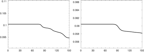
To verify the conservation properties of our scheme we run the tests for the streaming Weibel instability. The results are shown in Figure 1 for the mass and Figure 2 for the total energy. Both moments are very well conserved up to time $t\approx 70$ for case 1 and $t\approx 75$ for case 2, when the instabilities occur. After that the error for the mass is less then $2·{10}^{-4},$ however we can observe the large decay in the total energy.

Figure 1. Charge vs. time for case 1 (left) and case 2 (right) of the streaming Weibel instability.

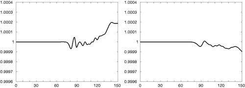
Figure 2. Total energy vs. time for case 1 (left) and case 2 (right) of the streaming Weibel instability.

7. Conclusions

This study is devoted to the hp streamline diffusion for the relativistic Vlasov–Maxwell system in 3 D. Our objective is to present space-time (for Maxwell’s) and phase-space-time (for VM system) discretization schemes that have optimal order of convergence ($\mathcal{O}\left({(h/p)}^{s+1/2}\right)$ for solutions in $H^{s+1}\left(\Omega \right)$), where h is the mesh size and p the spectral order. The adaptivity in a priori regime is based on refining in the vicinity of singularities combined with lower order approximating polynomials and nonrefined mesh with a higher spectral order in smooth regions. To our knowledge, except in some work in convection–diffusion problems, e.g. Asadzadeh and Sopasakis (2007), Houston et al. (2000), such approach is not considered elsewhere.

The results are justified, in lower dimensional cases, through the presented accuracy and the streaming Weibel instability tests. In all our simulations we used uniformly spaced grids in all variables and uniform degree of polynomials, and in the future paper we plan to examine the non-uniform grids and degree cases.

The full-dimensions are too complex and expensive to experiment. However, the theoretical analysis and numerical justifications in lower dimensions are indicating the robustness of the considered schemes.

References

- Asadzadeh, M., and A. Sopasakis. 2007. Convergence of a hp-streamline diffusion scheme for Vlasov–Fokker–Planck system. Math. Models Methods Appl. Sci. 17 (8): 1159–82. doi:10.1142/S0218202507002236
- Cheng, Y., I. M. Gamba, F. Li, and P. J. Morrison. 2014. Discontinuous Galerkin methods for the Vlasov–Maxwell equations. SIAM J. Numer. Anal. 52 (2): 1017–49. doi:10.1137/130915091
- DiPerna, R. J., and P. L. Lions. 1989. Global weak solutions of Vlasov–Maxwell systems. Comm. Pure Appl. Math. 42 (6): 729–57. doi:10.1002/cpa.3160420603
- Houston, P., C. Schwab, and E. Süli. 2000. Stabilized hp-finite element methods for first order hyperbolic problems, SIAM. SIAM J. Numer. Anal. 37 (5): 1618–43. doi:10.1137/S0036142998348777
- Schwab, C. 1998. p- and hp-Finite element methods. Theory and applications in solid and fluid mechanics. Oxford Science Publication.
- Standar, C. 2016. On streamline diffusion schemes for the one and one-half dimensional relativistic Vlasov–Maxwell system. Calcolo 53 (2): 147–69. doi:10.1007/s10092-015-0141-4