Linear Transport in Porous Media

Abstract

The linear transport theory is developed to describe the time dependence of the number density of tracer particles in porous media. The advection is taken into account. The transport equation is numerically solved by the analytical discrete ordinates method. For the inverse Laplace transform, the double-exponential formula is employed. In this paper, we consider the travel distance of tracer particles whereas the half-space geometry was assumed in our previous paper [Amagai et al. (2020). Trans. Porous Media 132:311–331].

Keywords:

• Boltzmann equation
• deterministic method
• transport equation

1. Introduction

The use of the transport equation for the flow in porous media was proposed by Williams (1992a, 1992b, 1993a, 1993b). Recently it was experimentally shown that the concentration of tracer particles in column experiments obeys the transport equation (Amagai et al. 2020). In Amagai et al. (2020), the advection u > 0 was taken into account. Then the spatial derivative term in the transport equation is given by $(u+v_0\mu )\partial /\partial x$ instead of $\mu \partial /\partial x,$ where $v_0>0$ is the inherent particle speed and $\mu \in [-1,1]$ is the cosine of the polar angle. The transport equation with such a spatial derivative term has been explored in the context of the evaporation of rarefied gas (Loyalka, Siewert, and Thomas 1981; Scherer and Barichello 2009; Siewert and Thomas 1981, 1982).

In column experiments (Cortis et al. 2004), a column tube is filled with a granular material such as sand or glass beads, and water is poured from the top end of the column. Then tracer particles are injected to the water. They enter the column from the top and eventually exit from the bottom of the column. In Amagai et al. (2020), the concentration of tracer particles was computed making use of the method of analytical discrete ordinates (ADO). Both the short-time growing behavior and long-time decay behavior of the breakthrough curve (the time dependence of the concentration) were well reproduced by the transport equation (Amagai et al. 2020).

In Amagai et al. (2020), the solution to the transport equation for a semi-infinite medium was compared to the experimental data. In this paper, we give a formulation for the transport equation in the slab geometry taking into account the length of the column. We make use of the double-exponential formula for the inverse Laplace transform.

The rest of the paper is organized as follows. In Section 2, we formulate our transport problem in the slab geometry. In Section 3, a numerical scheme is developed using ADO. In Section 4, our numerical scheme of the inverse Laplace transform is described. Finally, concluding remarks are given in Section 6.

2. The transport equation

Let us consider the one-dimensional linear Boltzmann equation. The velocity v is given by $v=u+v_0\mu .$ Let ${\sigma }_a>0$ and ${\sigma }_s>0$ be the absorption and scattering coefficients, respectively. Let L be the length of the column. We write our transport equation as follows. (2.1) $$\{\begin{array}{cc}\hfill & P\psi (x,\mu ,t)=\frac{{\sigma }_s}{2}{\int }_{-1}^1\psi (x,\mu ,t)d\mu ,\hspace{1em}0<x<L,\hspace{1em}-1\le \mu \le 1,\hspace{1em}t>0,\hfill \\ \hfill & \psi (x,\mu ,0)=0,\hspace{1em}0<x<L,\hspace{1em}-1\le \mu \le 1,\hfill \\ \hfill & \psi (0,\mu ,t)=n_0\delta (\mu -1),\hspace{1em}-\eta <\mu \le 1,\hspace{1em}t>0,\hfill \\ \hfill & \psi (L,\mu ,t)=0,\hspace{1em}-1\le \mu <-\eta ,\hspace{1em}t>0,\hfill \end{array}$$(2.1) where $$P\psi (x,\mu ,t)=\left[\frac{\partial }{\partial t}+(u+v_0\mu )\frac{\partial }{\partial x}+{\sigma }_a+{\sigma }_s\right]\psi (x,\mu ,t).$$

Here, $\delta (\mu -1)$ is the Dirac delta function, n₀ is the initial particle number density, and $$\eta =\frac{u}{v_0}.$$

We call $\psi (x,\mu ,t)$ the angular number density. The particle number density n(t) at x = L is given by $$n(t)={\int }_{-\eta }^1\psi (L,\mu ,t)d\mu .$$

3. The laplace transform

Let us introduce the Laplace transform $$\widehat{\psi }(x,\mu ,p)={\int }_0^{\infty }{e}^{-pt}\psi (x,\mu ,t)dt,\hspace{1em}p\in \mathbb{C},$$ and new variables $${\mu }_t=\frac{{\sigma }_a+{\sigma }_s+p}{v_0}\in \mathbb{C},\hspace{1em}{\mu }_s=\frac{{\sigma }_s}{v_0}>0.$$

Then we have $$\{\begin{array}{cc}\hfill & (\eta +\mu )\frac{\partial }{\partial x}\widehat{\psi }(x,\mu ,p)+{\mu }_t\widehat{\psi }(x,\mu ,p)=\frac{{\mu }_s}{2}{\int }_{-1}^1\widehat{\psi }(x,\mu ,p)d\mu ,\hspace{1em}0<x<L,\hspace{1em}-1\le \mu \le 1,\hfill \\ \hfill & \widehat{\psi }(0,\mu ,p)=\frac{n_0}{p}\delta (\mu -1),\hspace{1em}-\eta <\mu \le 1,\hfill \\ \hfill & \widehat{\psi }(L,\mu ,p)=0,\hspace{1em}-1\le \mu <-\eta .\hfill \end{array}$$

We note that the coefficient μ_t is a complex number and the boundary conditions are specified by intervals $(-\eta ,1]$ and $[-1,-\eta ).$ We will obtain $\widehat{\psi }(x,\mu ,p)$ in the above-mentioned equation using the analytical discrete ordinates method (ADO) (Barichello 2011; Barichello and Siewert 1999a, 1999b; Barichello, Garcia, and Siewert 2000; Barichello and Siewert 2001; Siewert and Wright 1999).

Remark 3.1.

By changing $\mu +\eta \to \tilde{\mu }$ and defining $\widehat{f}(x,\tilde{\mu },p)=\widehat{\psi }(x,\tilde{\mu }-\eta ,p),$ we can reformulate the equation as $$\{\begin{array}{cc}\hfill & \tilde{\mu }\frac{\partial }{\partial x}\widehat{f}(x,\tilde{\mu },p)+{\mu }_t\widehat{f}(x,\tilde{\mu },p)=\frac{{\mu }_s}{2}{\int }_{\eta -1}^{\eta +1}\widehat{f}(x,\tilde{\mu },p)d\tilde{\mu },\hspace{1em}0<x<L,\hspace{1em}\eta -1\le \tilde{\mu }\le \eta +1,\hfill \\ \hfill & \widehat{f}(0,\tilde{\mu },p)=\frac{n_0}{p}\delta (\tilde{\mu }-\eta -1),\hspace{1em}0<\tilde{\mu }\le \eta +1,\hfill \\ \hfill & \widehat{f}(L,\tilde{\mu },p)=0,\hspace{1em}\eta -1\le \tilde{\mu }<0,\hfill \end{array}$$

Such transformation is particularly useful for the evaporation problem, in which the integral on the right-hand side of the transport equation is taken from $-\infty$ to $\infty$ (Scherer and Barichello 2009).

Let us write $$\widehat{\psi }(x,\mu ,p)={\widehat{\psi }}_b(x,\mu ,p)+{\widehat{\psi }}_s(x,\mu ,p).$$

The ballistic term ${\widehat{\psi }}_b$ satisfies $$\{\begin{array}{cc}\hfill & (\eta +\mu )\frac{\partial }{\partial x}{\widehat{\psi }}_b(x,\mu ,p)+{\mu }_t{\widehat{\psi }}_b(x,\mu ,p)=0,\hspace{1em}0<x<L,\hspace{1em}-1\le \mu \le 1,\hfill \\ \hfill & {\widehat{\psi }}_b(0,\mu ,p)=\frac{n_0}{p}\delta (\mu -1),\hspace{1em}-\eta <\mu \le 1,\hfill \\ \hfill & {\widehat{\psi }}_b(L,\mu ,p)=0,\hspace{1em}-1\le \mu <-\eta ,\hfill \end{array}$$ and the scattering term ${\widehat{\psi }}_s$ obeys $$\{\begin{array}{cc}\hfill & \left[(\eta +\mu )\frac{\partial }{\partial x}+{\mu }_t\right]{\widehat{\psi }}_s=\frac{{\mu }_s}{2}{\int }_{-1}^1{\widehat{\psi }}_s(x,\mu ,p)d\mu +q,\hspace{1em}0<x<L,\hspace{1em}-1\le \mu \le 1,\hfill \\ \hfill & {\widehat{\psi }}_s(0,\mu ,p)=0,\hspace{1em}-\eta <\mu \le 1,\hfill \\ \hfill & {\widehat{\psi }}_s(L,\mu ,p)=0,\hspace{1em}-1\le \mu <-\eta ,\hfill \end{array}$$ where $$q(x,\mu ,p)=\frac{{\mu }_s}{2}{\int }_{-1}^1{\widehat{\psi }}_b(x,\mu ,p)d\mu =\frac{n_0{\mu }_s}{2p}{e}^{-x{\mu }_t/(\eta +1)}.$$

We note that $${\widehat{\psi }}_b(x,\mu ,p)=\frac{n_0}{p}{e}^{-x{\mu }_t/(\eta +\mu )}\delta (\mu -1).$$

Let us express ${\widehat{\psi }}_s(x,\mu ,p)={\widehat{\psi }}_s(x,\mu )$ and $q(x,\mu ,p)=q(x,\mu )$ when there is no confusion. For the computation of ${\widehat{\psi }}_s,$ we discretize the integral by the Gauss-Legendre quadrature and obtain $$\left[(\eta +{\mu }_i)\frac{\partial }{\partial x}+{\mu }_t\right]{\widehat{\psi }}_s(x,{\mu }_i)=\frac{{\mu }_s}{2}\sum _{j=1}^N{w}_j\left[{\widehat{\psi }}_s(x,{\mu }_j)+{\widehat{\psi }}_s(x,-{\mu }_j)\right]+q(x,{\mu }_i),$$ where ${\mu }_i,w_i$ ($i=1,2,\dots ,2N$) are abscissas and weights, respectively. We have $0<{\mu }_1<\cdots <{\mu }_N<1$ and ${\mu }_{N+i}=-{\mu }_i$ ($i=1,\dots ,N$). Furthermore, we introduce $N_{\eta }$ as the largest integer such that $-\eta <{\mu }_{N_{\eta }}.$

Remark 3.2.

It is possible to assign different abscissas and weights for two intervals $[-1,-\eta )$ and $(-\eta ,1].$ Since we assume η is small, we use one set of abscissas and weights for the interval $[-1,1]$ as described above.

The scattering part ${\widehat{\psi }}_s$ is obtained as $${\widehat{\psi }}_s(x,{\mu }_i)=\sum _{j=1}^{2N}{\int }_0^{L}G(x,{\mu }_i;x\prime ,{\mu }_j)q(x\prime ,{\mu }_j)dx\prime ,$$ where the Green’s function defined for each p satisfies $$\{\begin{array}{cc}\hfill & \left[(\eta +{\mu }_i)\frac{\partial }{\partial x}+{\mu }_t\right]G(x,{\mu }_i;x\prime ,{\mu }_j)=\frac{{\mu }_s}{2}\sum _{k=1}^{2N}{w}_{k}G(x,{\mu }_k;x\prime ,{\mu }_j)+\delta (x-x\prime ){\delta }_{ij},\hfill \\ \hfill & G(0,{\mu }_i;x\prime ,{\mu }_j)=0,\hspace{1em}{\mu }_i>{\mu }_{N_{\eta }},\hfill \\ \hfill & G(L,{\mu }_i;x\prime ,{\mu }_j)=0,\hspace{1em}{\mu }_i<{\mu }_{N_{\eta }},\hfill \end{array}$$ where δ_ij is the Kronecker delta.

Let us consider the following homogeneous equation. $$\left((\eta +{\mu }_i)\frac{\partial }{\partial x}+{\mu }_t\right)\widehat{\psi }(x,{\mu }_i)=\frac{{\mu }_s}{2}\sum _{j=1}^{2N}{w}_j\widehat{\psi }(x,{\mu }_j).$$

We note that $\widehat{\psi }$ depends on p through μ_t. With separation of variables, we can write $\widehat{\psi }$ as $$\widehat{\psi }(x,{\mu }_i)=\varphi (\nu ,{\mu }_i)e^{-x/\nu },$$ where ν is the separation constant. The function $\varphi (\nu ,{\mu }_i)$ satisfies the normalization condition, $$\sum _{i=1}^{2N}{w}_i\varphi (\nu ,{\mu }_i)=\sum _{i=1}^N{w}_i\left(\varphi (\nu ,{\mu }_i)+\varphi (\nu ,-{\mu }_i)\right)=1.$$

We obtain $$\varphi (\nu ,{\mu }_i)=\frac{{\mu }_s\nu }{2}\frac{1}{{\mu }_t\nu -{\mu }_i-\eta },$$ assuming $\nu \ne ({\mu }_i+\eta )/{\mu }_t.$ If η = 0 and p is real, we can prove $\nu \ne {\mu }_i/{\mu }_t$ (Siewert and Wright 1999). The following orthogonality relation holds. $$\sum _{i=1}^{2N}{w}_i({\mu }_i+\eta )\varphi (\nu ,{\mu }_i)\varphi (\nu \prime ,{\mu }_i)=\mathcal{N}(\nu ){\delta }_{\nu \nu \prime },$$ where $$\mathcal{N}(\nu )=\sum _{i=1}^{2N}{w}_i({\mu }_i+\eta )\varphi {(\nu ,{\mu }_i)}^2.$$

We can find 2 N eigenvalues $\nu ={\nu }_n$ ($n=1,2,\dots ,2N$). The eigenvalues can be obtained as the reciprocal of eigenvalues of the following matrix (Amagai et al. 2020). $$\left(\begin{array}{cc}{\Xi }_{+}^{-1}& \\ & {\Xi }_{-}^{-1}\end{array}\right)\left[{\mu }_t\left(\begin{array}{cc}I& \\ & I\end{array}\right)-\frac{{\mu }_s}{2}\left(\begin{array}{cc}W& W\\ W& W\end{array}\right)\right],$$ where I is the identity, ${\Xi }_{\pm }=\text{diag}(\pm {\mu }_1+\eta ,\pm {\mu }_2+\eta ,\dots ,\pm {\mu }_N+\eta ),$ and ${\left\{W\right\}}_{ij}=w_j.$ The subroutine ZGEEV (LAPACK subroutine for a complex nonsymmetric matrix) was used to compute ν_n. Moreover, the free-space Green’s function G₀ is obtained as $$G_0(x,{\mu }_i;x\prime ,{\mu }_j)=\pm \sum _{\pm \mathfrak{R}{\nu }_n>0}\frac{w_j}{\mathcal{N}({\nu }_n)}\varphi ({\nu }_n,{\mu }_j)\varphi ({\nu }_n,{\mu }_i)e^{-(x-x\prime )/{\nu }_n},$$ where upper signs are chosen for $x>x\prime$ and lower signs are used for $x<x\prime .$

Hence we can write $$\begin{array}{cc}G(x,{\mu }_i;x\prime ,{\mu }_j)\hfill & =G_0(x,{\mu }_i;x\prime ,{\mu }_j)\hfill \\ \hfill & +\sum _{\mathfrak{R}{\nu }_n>0}{B}_1({\nu }_n)\varphi ({\nu }_n,{\mu }_i)e^{-x/{\nu }_n}+\sum _{\mathfrak{R}{\nu }_n<0}{B}_2({\nu }_n)\varphi ({\nu }_n,{\mu }_i)e^{-x/{\nu }_n},\hfill \end{array}$$ where coefficients $B_1({\nu }_n),B_2({\nu }_n)$ are determined from boundary conditions. We obtain (3.1) $$\sum _{\mathfrak{R}{\nu }_n>0}{B}_1({\nu }_n)\varphi ({\nu }_n,{\mu }_{i_1})+\sum _{\mathfrak{R}{\nu }_n<0}{B}_2({\nu }_n)\varphi ({\nu }_n,{\mu }_{i_1})=y_1({\mu }_{i_1}),$$(3.1) (3.2) $$\sum _{\mathfrak{R}{\nu }_n>0}{B}_1({\nu }_n)\varphi ({\nu }_n,{\mu }_{i_2})e^{-L/{\nu }_n}+\sum _{\mathfrak{R}{\nu }_n<0}{B}_2({\nu }_n)\varphi ({\nu }_n,{\mu }_{i_2})e^{-L/{\nu }_n}=y_2({\mu }_{i_2}),$$(3.2) where $1\le i_1\le N_{\eta },N_{\eta }<i_2\le 2N,$ $$\begin{array}{cc}{y}_1({\mu }_{i_1})\hfill & =\sum _{\mathfrak{R}{\nu }_n<0}\frac{w_j}{\mathcal{N}({\nu }_n)}\varphi ({\nu }_n,{\mu }_j)\varphi ({\nu }_n,{\mu }_{i_1})e^{x^{\prime }/{\nu }_n},\hfill \\ y_2({\mu }_{i_2})\hfill & =-\sum _{\mathfrak{R}{\nu }_n>0}\frac{w_j}{\mathcal{N}({\nu }_n)}\varphi ({\nu }_n,{\mu }_j)\varphi ({\nu }_n,{\mu }_{i_2})e^{-(L-x\prime )/{\nu }_n}.\hfill \end{array}$$

Let us multiply (3.1)(3.1) $$\sum _{\mathfrak{R}{\nu }_n>0}{B}_1({\nu }_n)\varphi ({\nu }_n,{\mu }_{i_1})+\sum _{\mathfrak{R}{\nu }_n<0}{B}_2({\nu }_n)\varphi ({\nu }_n,{\mu }_{i_1})=y_1({\mu }_{i_1}),$$(3.1) and (3.2)(3.2) $$\sum _{\mathfrak{R}{\nu }_n>0}{B}_1({\nu }_n)\varphi ({\nu }_n,{\mu }_{i_2})e^{-L/{\nu }_n}+\sum _{\mathfrak{R}{\nu }_n<0}{B}_2({\nu }_n)\varphi ({\nu }_n,{\mu }_{i_2})e^{-L/{\nu }_n}=y_2({\mu }_{i_2}),$$(3.2) by $\text{exp}\hspace{0.17em}(-x\prime {\mu }_t/(\eta +1)),$ integrate both sides of these equations over $x\prime ,$ and take the sum with respect to j. We obtain (3.3) $$\sum _{\mathfrak{R}{\nu }_n>0}{E}_1({\nu }_n)\varphi ({\nu }_n,{\mu }_{i_1})+\sum _{\mathfrak{R}{\nu }_n<0}{E}_2({\nu }_n)\varphi ({\nu }_n,{\mu }_{i_1})e^{L/{\nu }_n}=z_1({\mu }_{i_1}),$$(3.3) (3.4) $$\sum _{\mathfrak{R}{\nu }_n>0}{E}_1({\nu }_n)\varphi ({\nu }_n,{\mu }_{i_2})e^{-L/{\nu }_n}+\sum _{\mathfrak{R}{\nu }_n<0}{E}_2({\nu }_n)\varphi ({\nu }_n,{\mu }_{i_2})=z_2({\mu }_{i_2}),$$(3.4) where $$\begin{array}{cc}{z}_1({\mu }_{i_1})\hfill & =\sum _{\mathfrak{R}{\nu }_n<0}\frac{(\eta +1){\nu }_n}{\mathcal{N}({\nu }_n)(\eta +1-{\nu }_n{\mu }_t)}\left[e^{L/{\nu }_n-L{\mu }_t/(\eta +1)}-1\right]\varphi ({\nu }_n,{\mu }_{i_1}),\hfill \\ z_2({\mu }_{i_2})\hfill & =\sum _{\mathfrak{R}{\nu }_n>0}\frac{(\eta +1){\nu }_n}{\mathcal{N}({\nu }_n)(\eta +1-{\nu }_n{\mu }_t)}\left[e^{-L{\mu }_t/(\eta +1)}-e^{-L/{\nu }_n}\right]\varphi ({\nu }_n,{\mu }_{i_2}),\hfill \end{array}$$ and $$\{\begin{array}{cc}{E}_1({\nu }_n)\hfill & =\sum _{j=1}^{2N}{\int }_0^L{B}_1({\nu }_n)e^{-{\mu }_{t}x\prime /(\eta +1)}dx\prime ,\hfill \\ E_2({\nu }_n)\hfill & =e^{-L/{\nu }_n}\sum _{j=1}^{2N}{\int }_0^L{B}_2({\nu }_n)e^{-{\mu }_{t}x\prime /(\eta +1)}dx\prime .\hfill \end{array}$$

Thus $E_1({\nu }_n),E_2({\nu }_n)$ are obtained from (3.3)(3.3) $$\sum _{\mathfrak{R}{\nu }_n>0}{E}_1({\nu }_n)\varphi ({\nu }_n,{\mu }_{i_1})+\sum _{\mathfrak{R}{\nu }_n<0}{E}_2({\nu }_n)\varphi ({\nu }_n,{\mu }_{i_1})e^{L/{\nu }_n}=z_1({\mu }_{i_1}),$$(3.3) and (3.4)(3.4) $$\sum _{\mathfrak{R}{\nu }_n>0}{E}_1({\nu }_n)\varphi ({\nu }_n,{\mu }_{i_2})e^{-L/{\nu }_n}+\sum _{\mathfrak{R}{\nu }_n<0}{E}_2({\nu }_n)\varphi ({\nu }_n,{\mu }_{i_2})=z_2({\mu }_{i_2}),$$(3.4) . To solve this linear system, the subroutine ZGESV (LAPACK subroutine for a complex system of linear equations) was used.

Hence we obtain $$\begin{array}{cc}{\widehat{\psi }}_s(x,{\mu }_i)\hfill & =\frac{n_0{\mu }_s}{2p}\sum _{j=1}^{2N}{\int }_0^{L}G(x,{\mu }_i;x\prime ,{\mu }_j)e^{-x\prime {\mu }_t/(\eta +1)}dx\prime \hfill \\ \hfill & =\frac{n_0{\mu }_s}{2p}\sum _{\mathfrak{R}{\nu }_n>0}\frac{(\eta +1){\nu }_n}{\mathcal{N}({\nu }_n)(\eta +1-{\nu }_n{\mu }_t)}\left(e^{-{\mu }_{t}x/(\eta +1)}-e^{-x/{\nu }_n}\right)\varphi ({\nu }_n,{\mu }_i)\hfill \\ \hfill & +\frac{n_0{\mu }_s}{2p}\sum _{\mathfrak{R}{\nu }_n<0}\frac{(\eta +1){\nu }_n}{\mathcal{N}({\nu }_n)(\eta +1-{\nu }_n{\mu }_t)}{e}^{-x{\mu }_t/(\eta +1)}\left(1-e^{(L-x)/{\nu }_n-(L-x){\mu }_t/(\eta +1)}\right)\varphi ({\nu }_n,{\mu }_i)\hfill \\ \hfill & +\frac{n_0{\mu }_s}{2p}\left[\sum _{\mathfrak{R}{\nu }_n>0}{E}_1({\nu }_n)\varphi ({\nu }_n,{\mu }_i)e^{-x/{\nu }_n}+\sum _{\mathfrak{R}{\nu }_n<0}{E}_2({\nu }_n)\varphi ({\nu }_n,{\mu }_i)e^{(L-x)/{\nu }_n}\right].\hfill \end{array}$$

The Laplace transform of n(t) is obtained as $$\begin{array}{cc}\widehat{n}(p)\hfill & ={\int }_{-\eta }^1\widehat{\psi }(L,\mu ,p)d\mu \hfill \\ \hfill & ={\int }_{-\eta }^1{\widehat{\psi }}_b(L,\mu ,p)d\mu +{\int }_{-\eta }^1{\widehat{\psi }}_s(L,\mu ,p)d\mu .\hfill \end{array}$$

Therefore, $$\begin{array}{cc}\widehat{n}(p)\hfill & =\frac{n_0}{p}{e}^{-L{\mu }_t/(\eta +1)}\hfill \\ \hfill & +\frac{n_0{\mu }_s}{2p}\sum _{\mathfrak{R}{\nu }_n>0}\frac{(\eta +1){\nu }_n}{\mathcal{N}({\nu }_n)(\eta +1-{\nu }_n{\mu }_t)}\left(e^{-L{\mu }_t/(\eta +1)}-e^{-L/{\nu }_n}\right)\phi ({\nu }_n)\hfill \\ \hfill & +\frac{n_0{\mu }_s}{2p}\left[\sum _{\mathfrak{R}{\nu }_n>0}{E}_1({\nu }_n)e^{-L/{\nu }_n}\phi ({\nu }_n)+\sum _{\mathfrak{R}{\nu }_n<0}{E}_2({\nu }_n)\phi ({\nu }_n)\right],\hfill \end{array}$$ where $$\phi (\nu )=\sum _{i=1}^{N_{\eta }}{w}_i\varphi (\nu ,{\mu }_i)=\frac{{\mu }_s\nu }{2}\sum _{i=1}^{N_{\eta }}\frac{w_i}{{\mu }_t\nu -{\mu }_i-\eta }.$$

By the inverse Laplace transform, we have (3.5) $$\begin{array}{cc}n(t)\hfill & =\frac{n_0}{2\pi i}{\int }_{\gamma -i\infty }^{\gamma +i\infty }\frac{e^{pt}}{p}\{e^{-L{\mu }_t/(\eta +1)}\hfill \\ \hfill & +\frac{{\mu }_s}{2}\sum _{\mathfrak{R}{\nu }_n>0}\frac{(\eta +1){\nu }_n}{\mathcal{N}({\nu }_n)(\eta +1-{\nu }_n{\mu }_t)}\left(e^{-L{\mu }_t/(\eta +1)}-e^{-L/{\nu }_n}\right)\phi ({\nu }_n)\hfill \\ \hfill & +\frac{{\mu }_s}{2}[\sum _{\mathfrak{R}{\nu }_n>0}{E}_1({\nu }_n)e^{-L/{\nu }_n}\phi ({\nu }_n)+\sum _{\mathfrak{R}{\nu }_n<0}{E}_2({\nu }_n)\phi ({\nu }_n)]\}dp,\hfill \end{array}$$(3.5) where γ is taken to be greater than the largest real part of any singularity.

4. The inverse Laplace transform

Let us numerically evaluate the Bromwich integral in the inverse Laplace transform (3.5)(3.5) $$\begin{array}{cc}n(t)\hfill & =\frac{n_0}{2\pi i}{\int }_{\gamma -i\infty }^{\gamma +i\infty }\frac{e^{pt}}{p}\{e^{-L{\mu }_t/(\eta +1)}\hfill \\ \hfill & +\frac{{\mu }_s}{2}\sum _{\mathfrak{R}{\nu }_n>0}\frac{(\eta +1){\nu }_n}{\mathcal{N}({\nu }_n)(\eta +1-{\nu }_n{\mu }_t)}\left(e^{-L{\mu }_t/(\eta +1)}-e^{-L/{\nu }_n}\right)\phi ({\nu }_n)\hfill \\ \hfill & +\frac{{\mu }_s}{2}[\sum _{\mathfrak{R}{\nu }_n>0}{E}_1({\nu }_n)e^{-L/{\nu }_n}\phi ({\nu }_n)+\sum _{\mathfrak{R}{\nu }_n<0}{E}_2({\nu }_n)\phi ({\nu }_n)]\}dp,\hfill \end{array}$$(3.5) . Although the trapezoidal rule was used in Amagai et al. (2020), here we employed the double-exponential formula (Ooura and Mori 1991, 1999).

We note that $\mathfrak{I}\widehat{n}(\gamma +i\omega /t)=-\mathfrak{R}\widehat{n}(\gamma +i(\omega -\frac{\pi }{2})/t)$ because $$\widehat{n}\left(\gamma +i\frac{\omega -\frac{\pi }{2}}{t}\right)={\int }_0^{\infty }{e}^{-\gamma t-i(\omega -\frac{\pi }{2})}n(t)dt=i\widehat{n}\left(\gamma +i\frac{\omega }{t}\right).$$

For t > 0, we have (4.1) $$\begin{array}{cc}n(t)\hfill & =\frac{e^{\gamma t}}{2\pi t}{\int }_{-\infty }^{\infty }{e}^{i\omega }\widehat{n}\left(\gamma +i\frac{\omega }{t}\right)d\omega =\frac{e^{\gamma t}}{\pi t}{\int }_{-\infty }^{\infty }\hspace{0.17em}\text{cos}\hspace{0.17em}\omega \mathfrak{R}\widehat{n}\left(\gamma +i\frac{\omega }{t}\right)d\omega \hfill \\ \hfill & =\frac{2e^{\gamma t}}{\pi t}{\int }_0^{\infty }\hspace{0.17em}\text{cos}\hspace{0.17em}\omega \mathfrak{R}\widehat{n}\left(\gamma +\frac{i\omega }{t}\right)d\omega .\hfill \end{array}$$(4.1)

Let us introduce (4.2) $$\varphi (\tau )=\frac{\tau }{1-e^{-K\mathrm{\hspace{0.17em}sinh}\tau }},\hspace{1em}K=6.$$(4.2)

Then the above integral can be written as $$n(t)=\frac{2e^{\gamma t}}{\pi t}{\int }_{-\infty }^{\infty }\hspace{0.17em}\text{cos}\hspace{0.17em}(M\varphi (\tau ))\mathfrak{R}\widehat{n}\left(\gamma +\frac{i}{t}M\varphi (\tau )\right)M\frac{d}{d\tau }\varphi (\tau )d\tau ,$$ where $\omega =M\varphi (\tau ),$ M > 0. Let us define $h=\pi /M.$ To numerically evaluate the above integral, the discretization by the trapezoidal rule is the suitable choice (Sugihara 1997; Trefethen and Weideman 2014). By the trapezoidal rule, we arrive at (4.3) $$n(t)\approx \frac{2e^{\gamma t}}{t}\sum _{k=-k_{\text{max}}}^{k_{\text{max}}}\hspace{0.17em}\text{cos}\hspace{0.17em}\left(M\varphi (\tau )\right)\mathfrak{R}\widehat{n}\left(\gamma +\frac{iM}{t}\varphi (\tau )\right)\varphi \prime (\tau ),$$(4.3) where $k_{\text{max}}$ is an integer and $\tau =kh+\frac{\pi }{2M}.$ We note that $\varphi \prime (\tau )\to 0$ double exponentially as $\tau \to -\infty .$ We see that $\varphi (\tau )\to \tau$ double exponentially as $\tau \to \infty$ and $\text{cos}\hspace{0.17em}(M\varphi (kh+\frac{\pi }{2M}))\sim \hspace{0.17em}\text{cos}\hspace{0.17em}(\mathit{Mkh}+\frac{\pi }{2})=0.$ The choice of $\varphi (\tau )$ in (4.2)(4.2) $$\varphi (\tau )=\frac{\tau }{1-e^{-K\mathrm{\hspace{0.17em}sinh}\tau }},\hspace{1em}K=6.$$(4.2) is not unique. The constant K = 6 was found by numerical experiments (Ooura and Mori 1991). In Table A1 in Appendix A, we confirmed that any $K\approx 6$ gives the same numerical results. Although $\varphi (\tau )$ in (4.2)(4.2) $$\varphi (\tau )=\frac{\tau }{1-e^{-K\mathrm{\hspace{0.17em}sinh}\tau }},\hspace{1em}K=6.$$(4.2) sufficiently works, a more general expression $\varphi (\tau )=\tau {[1-\hspace{0.17em}\text{exp}\hspace{0.17em}(-2\tau -\alpha (1-e^{-\tau })-\beta (e^{\tau }-1))]}^{-1}$ ($\beta =1/4,\alpha =\beta /\sqrt{1+M\hspace{0.17em}\text{ln}\hspace{0.17em}(1+M)/(4\pi )}$) has been proposed (Ooura and Mori 1999).

Table A1. The dependence of $n(L,t)/n_0$ on K for N = 30, $k_{\text{max}}=40,$ M = 40.

$K\backslash t$	$5\text{min}$	$10\text{min}$	$15\text{min}$	$20\text{min}$
0.6	−0.0451	2.77	3.59	3.79
1	1.36	3.72	4.39	4.52
2	1.38	3.73	4.39	4.53
6	1.38	3.73	4.39	4.53
10	1.38	3.73	4.39	4.53
20	1.37	3.74	4.39	4.52
30	1.49	3.71	4.33	4.52
60	3.88	4.12	3.62	3.26

Table A2. The dependence of $n(L,t)/n_0$ on N for K = 6, $k_{\text{max}}=40,$ M = 40.

$N\backslash t$	$5\text{min}$	$10\text{min}$	$15\text{min}$	$20\text{min}$
5	1.65	4.35	5.09	5.23
10	1.33	3.64	4.30	4.44
15	1.38	3.74	4.41	4.54
20	1.38	3.74	4.40	4.53
25	1.38	3.73	4.40	4.53
30	1.38	3.73	4.39	4.53
35	1.38	3.73	4.39	4.53

We set $L=10\text{cm}.$ We found $\gamma =0.04$ is suitable. Time was discretized as $t_j=j\Delta t$ ($\Delta t=0.2\text{min},j=1,\dots ,250$). Furthermore we set ${\sigma }_a={10}^{-8}{\text{min}}^{-1},{\sigma }_s=5{\text{min}}^{-1},v_0=5\text{cm}/\text{min},$ and $u=1.5\text{cm}/\text{min}.$ For the numerical calculation, parameters were chosen to be N = 30, $k_{\text{max}}=40,$ and $M=40.$ To confirm the validity of these values, Tables A2–A4 in Appendix A compare $n(L,t)/n_0$ for different parameters.The computation time was $90\hspace{0.17em}\text{sec}\hspace{0.17em}$ on a laptop computer (MacBook Pro, 2.3 GHz Intel Core i5). The result is plotted in Figure 1. In Amagai et al. (2020), the particle number density was defined by (4.4) $$n(x,t)={\int }_{-1}^1{\psi }_{\infty }(x,\mu ,t)d\mu ,$$(4.4) where ${\psi }_{\infty }(x,\mu ,t)$ is the solution to (2.1)(2.1) $$\{\begin{array}{cc}\hfill & P\psi (x,\mu ,t)=\frac{{\sigma }_s}{2}{\int }_{-1}^1\psi (x,\mu ,t)d\mu ,\hspace{1em}0<x<L,\hspace{1em}-1\le \mu \le 1,\hspace{1em}t>0,\hfill \\ \hfill & \psi (x,\mu ,0)=0,\hspace{1em}0<x<L,\hspace{1em}-1\le \mu \le 1,\hfill \\ \hfill & \psi (0,\mu ,t)=n_0\delta (\mu -1),\hspace{1em}-\eta <\mu \le 1,\hspace{1em}t>0,\hfill \\ \hfill & \psi (L,\mu ,t)=0,\hspace{1em}-1\le \mu <-\eta ,\hspace{1em}t>0,\hfill \end{array}$$(2.1) when $L\to \infty .$ Figure 1 also shows $n(L,t)/n_0$ for comparison.

Figure 1. The particle number density is plotted as a function of t. The blue curve is from (4.3) and the red curve is from (4.4).

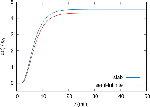
Table A3. The dependence of $n(L,t)/n_0$ on $k_{\text{max}}$ for K = 6, N = 30, M = 40.

$k_{\text{max}}$\t	$5\text{min}$	$10\text{min}$	$15\text{min}$	$20\text{min}$
10	−0.40	2.43	3.30	3.51
20	1.38	3.73	4.39	4.53
30	1.38	3.73	4.39	4.53
40	1.38	3.73	4.39	4.53
50	1.38	3.73	4.39	4.53

Table A4. The dependence of $n(L,t)/n_0$ on M for K = 6, N = 30, $k_{\text{max}}=40.$

M\t	$5\text{min}$	$10\text{min}$	$15\text{min}$	$20\text{min}$
30	1.38	3.73	4.39	4.53
40	1.38	3.73	4.39	4.53
50	1.38	3.73	4.39	4.53
60	1.38	3.73	4.39	4.53

To confirm the convergence of the inverse Laplace transform, we have tried different N, $k_{\text{max}},$ and M.

Remark 4.1.

According to the error analysis in Ganapol (2008), γt must be small. In Ganapol (2008), it is suggested to move γ according to t, and the form $\gamma =\overline{\gamma }+\alpha /t$ is proposed, where $\overline{\gamma },\alpha$ are positive constants.

5. Column experiment

A one-dimensional flow field is achieved in a column. We conducted a column experiment using adsorptive solute of zinc solution.

Before the tracer breakthrough curve was observed, ultra-pure water was injected by the peristaltic pump (MP-1000, Eyela) for 24 hours until the flow field became steady. The flow rate of the injected tracer solution was controlled by the peristaltic pump. Then the tracer solution was injected to displace the fresh water. The discharged solution was collected by the fraction collector (CHF161RA, Advantec) at regular intervals. Column experiments were performed at room temperature of 25–$26°\mathrm{C}.$ The experiment was conducted until the discharge concentration became equal to the influent concentration. For the sake of the accuracy of measurements, we corrected the measurement time error from the tube volume and inlet volume of the column by subtracting the time lag due to the switchover from the breakthrough time.

The filling material is the standard sand (Tohoku silica sand No. 4, Kitanihon Sangyo). The median diameter of the sand is $750\mu \mathrm{m}.$ As a preparation, we eliminate the organic matter that may have been contained in the sand by soaking it in ${\text{HNO}}_3$ solution. The zinc solution was $2\text{ppm}.$ We set a filter on the top of the sand bed made with glass wool and put the same filter at the bottom of the column. A column of length $12.0\text{cm}$ with internal diameter 3.1 cm was used. The bed height was $L=10.7\text{cm}$ and the section area was $7.54{\text{cm}}^2.$ It was confirmed by a blank test that the zinc was not absorbed on the surface of the column wall. The concentration was measured with the atomic absorption photometer (Z-2300, Hitachi High-Technologies), the compressor (SC820, Koki Holdings), and the Neo Cool Circulator (CF700, Yamato). The measured porosity was 0.289 and the flow rate was $11.25{\text{cm}}^3/\mathrm{h}.$

Figure 2 shows the zinc breakthrough curve. The measured values from the column experiment (black open circles) are compared with numerical values calculated from (4.3)(4.3) $$n(t)\approx \frac{2e^{\gamma t}}{t}\sum _{k=-k_{\text{max}}}^{k_{\text{max}}}\hspace{0.17em}\text{cos}\hspace{0.17em}\left(M\varphi (\tau )\right)\mathfrak{R}\widehat{n}\left(\gamma +\frac{iM}{t}\varphi (\tau )\right)\varphi \prime (\tau ),$$(4.3) and (4.4)(4.4) $$n(x,t)={\int }_{-1}^1{\psi }_{\infty }(x,\mu ,t)d\mu ,$$(4.4) using the linear transport equation in the slab geometry (blue dashed line) and half-space geometry (red line). In the left panel of Figure 2, the vertical axis is the relative concentration $C/C_0$ and the horizontal axis is time t. The semilog plot in the right panel of Figure 2 shows $1-C/C_0$ as a function of t. When numerically obtaining $C/C_0,$ we determined the parameters by the Levenberg-Marquardt algorithm (Levenberg 1944; Marquardt 1963) using the FORTRAN library MINPACK (More, Garbow, and Hillstrom 1980). The fitted values are summarized in Table 1. The parameter values for the half space in Table 1 were obtained in Amagai et al. (2020). We note that $C/C_0$ and $n/n_0$ are related as $C/C_0=\beta n/n_0$ with constant β, which is determined by fitting. We see in Figure 2 that two curves from the transport equation are almost identical with different parameter values.

Figure 2. The breakthrough curve of $C/C_0$ (Left) and $1-C/C_0$ (Right) as a function of time. The experimental data (black open circles) are compared with numerical values computed from (4.3) and (4.4) using the linear transport equation in the slab geometry (blue dashed line) and half-space geometry (red line).

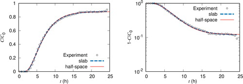
Table 1. Fitted parameters.

	σs (${\mathrm{h}}^{-1}$)	v0 ($\text{cm}/\mathrm{h}$)	u ($\text{cm}/\mathrm{h}$)	β
slab	1.98	3.31	1.52	0.25
half space	2.68	4.12	1.80	0.21

6. Concluding remarks

Although solutions of the transport equation well described experimentally obtained breakthrough curves in Amagai et al. (2020), the half space was assumed in the formulation. To take into account the length of the column, we gave a formulation in the slab geometry, which has both ends and tracer particles enter from one end and exit from the other end. It should be emphasized that indistinguishable breakthrough curves are obtained for different sets of fitted parameters. This means that it is important to impose the boundary conditions which correctly model the experimental setup.

For the numerical inversion of the Laplace transform, we could apply the double-exponential formula after expressing n(t) using $\text{cos}\hspace{0.17em}\omega$ in (4.1)(4.1) $$\begin{array}{cc}n(t)\hfill & =\frac{e^{\gamma t}}{2\pi t}{\int }_{-\infty }^{\infty }{e}^{i\omega }\widehat{n}\left(\gamma +i\frac{\omega }{t}\right)d\omega =\frac{e^{\gamma t}}{\pi t}{\int }_{-\infty }^{\infty }\hspace{0.17em}\text{cos}\hspace{0.17em}\omega \mathfrak{R}\widehat{n}\left(\gamma +i\frac{\omega }{t}\right)d\omega \hfill \\ \hfill & =\frac{2e^{\gamma t}}{\pi t}{\int }_0^{\infty }\hspace{0.17em}\text{cos}\hspace{0.17em}\omega \mathfrak{R}\widehat{n}\left(\gamma +\frac{i\omega }{t}\right)d\omega .\hfill \end{array}$$(4.1) .

In this paper, isotropic scattering is assumed. The introduction of the anisotropy factor $\mathrm{g}\ne 0$ is a future issue.

The most precise geometry for the column experiment is a cylinder in three dimensions. However, the essential nature of the transport is expected to be seen by the one-dimensional transport equation since the experimental setup is designed so that the flow is identical in horizontal directions.

Acknowledgment

The column experiment was conducted by Motoko Yamakawa.

Additional information

Funding

M.M. acknowledges support from Grant-in-Aid for Scientific Research (17K05572, 18K03438) of JSPS.

Appendix A.

Parameters for numerical calculation

References

- Amagai, K., M. Yamakawa, M. Machida, and Y. Hatano. 2020. The linear Boltzmann equation in column experiments of porous media. Transp. Porous Med. 132 (2):311–31.
- Barichello, L. B. 2011. Explicit formulations for radiative transfer problems. In Thermal measurements and inverse techniques, ed. H. R. B. Orlande, O. Fudym, D. Maillet, and R. M. Cotta. Boca Raton, FL: CRS Press.
- Barichello, L. B., and C. E. Siewert. 1999a. A discrete-ordinates solution for a non-grey model with complete frequency redistribution. J. Quant. Spec. Rad. Trans. 62 (6):665–75.
- Barichello, L. B., and C. E. Siewert. 1999b. A discrete-ordinates solution for a polarization model with complete frequency redistribution. Astro. J. 513 (1):370–82.
- Barichello, L. B., and C. E. Siewert. 2001. A new version of the discrete-ordinates method. Proceedings 2 International Conference on Computational Heat and Mass Transfer, Rio de Janeiro, 22–26.
- Barichello, L. B., R. D. M. Garcia, and C. E. Siewert. 2000. Particular solutions for the discrete-ordinates method. J. Quant. Spec. Rad. Trans. 64 (3):219–26.
- Cortis, A., Y. Chen, H. Scher, and B. Berkowitz. 2004. Quantitative characterization of pore-scale disorder effects on transport in “homogeneous” granular media. Phys. Rev. E Stat. Nonlin. Soft Matter Phys. 70 (4 Pt 1):041108. doi:https://doi.org/10.1103/PhysRevE.70.041108
- Ganapol, B. D. 2008. Analytical benchmarks for nuclear engineering applications case studies in neutron transport theory. Paris: Nuclear Energy Agency, OECD.
- Levenberg, K. 1944. A method for the solution of certain non-linear problems in least squares. Quart. Appl. Math. 2 (2):164–8.
- Loyalka, S. K., C. E. Siewert, and J. R. Thomas. Jr., 1981. An approximate solution concerning strong evaporation into a half space. Z. Angew. Math. Phys. 32 (6):745–7.
- Marquardt, D. W. 1963. An algorithm for least-squares estimation of nonlinear parameters. SIAM J. Appl. Math. 11 (2):431–41.
- More, J. J., B. S. Garbow, and K. E. Hillstrom. 1980. User guide for MINPACK-1. Argonne National Laboratory Report ANL-80-74.
- Ooura, T., and M. Mori. 1991. The double exponential formula for oscillatory functions over the half infinite interval. J. Comp. Appl. Math 38 (1-3):353–60.
- Ooura, T., and M. Mori. 1999. A robust double exponential formula for Fourier-type integrals. J. Comp. Appl. Math. 112 (1–2):229–41.
- Scherer, C. S., and L. B. Barichello. 2009. Evaporation effects in rarefied gas flows. Proc. COBEM 2009 COB09:0684.
- Siewert, C. E. 2000. A concise and accurate solution to Chandrasekhar’s basic problem in radiative transfer. J. Quant. Spec. Rad. Trans. 64 (2):109–30.
- Siewert, C. E., and J. R. Thomas Jr. 1981. Strong evaporation into a half space. Z. Angew. Math. Phys. 32 (4):421–33.
- Siewert, C. E., and J. R. Thomas Jr. 1982. Strong evaporation into a half space. II. The three dimensional BGK model. Z. Angew. Math. Phys. 33 (2):202–18.
- Siewert, C. E., and S. J. Wright. 1999. Efficient eigenvalue calculations in radiative transfer. J. Quant. Spec. Rad. Trans. 62 (6):685–8.
- Sugihara, M. 1997. Optimality of the double exponential formula – functional analysis approach. Num. Math. 75 (3):379–95.
- Trefethen, L. N., and J. A. C. Weideman. 2014. The exponentially convergent trapezoidal rule. SIAM Rev. 56 (3):385–458.
- Williams, M. M. R. 1992. A new model for describing the transport of radionuclides through fractured rock. Ann. Nucl. Energy 19 (10–12):791–824.
- Williams, M. M. R. 1992. Stochastic problems in the transport of radioactive nuclides in fractured rock. Nucl. Sci. Eng. 112 (3):215–30.
- Williams, M. M. R. 1993. A new model for describing the transport of radionuclides through fractured rock Part II: Numerical results. Ann. Nucl. Energy 20 (3):185–202.
- Williams, M. M. R. 1993. Radionuclide transport in fractured rock a new model: Application and discussion. Ann. Nucl. Energy 20 (4):279–97.