Modified Fokker-Planck Acceleration for Forward-Peaked Transport Problems in Slab Geometry

Abstract

This paper introduces a new acceleration technique for the convergence of the solution of transport problems with highly forward-peaked scattering. The technique is similar to a conventional high-order/low-order (HOLO) acceleration scheme. The Fokker-Planck equation, which is an asymptotic limit of the transport equation in highly forward-peaked settings, is modified and used for acceleration; this modified equation preserves the angular flux and moments of the (high-order) transport equation. We present numerical results using the Screened Rutherford, Exponential, and Henyey–Greenstein scattering kernels and compare them to established acceleration methods such as diffusion synthetic acceleration (DSA). We observe three to four orders of magnitude speed-up in wall-clock time compared to DSA.

Keywords:

• Fokker-Planck
• transport
• HOLO
• forward-peaked scattering

1. Introduction

Transport problems with highly forward-peaked scattering are prevalent in a variety of areas, including astrophysics, medical physics, and plasma physics (Henyey and Greenstein 1941; Aristova and Gol'din 2000; Patel et al. 2019). For these problems, solutions of the transport equation converge slowly when using conventional methods such as source iteration (SI) (Adams and Larsen 2002) and the generalized minimal residual method (GMRES) (Saad and Schultz 1986). Moreover, diffusion-based acceleration techniques like diffusion synthetic acceleration (DSA) (Alcouffe 1977) and nonlinear diffusion acceleration (NDA) (Knoll et al. 2011) are generally inefficient when tackling these problems, as they only accelerate up to the first moment of the angular flux (Patel et al. 2020). Higher order moments carry important information in problems with highly forward-peaked scattering and can be used to further accelerate convergence (Patel 2016).

This paper focuses on solution methods for the monoenergetic, steady-state transport equation in slab geometry. Under these conditions, the transport equation is given by: (1.1a) $$\mu \frac{\partial }{\partial x}\psi (x,\mu )+{\sigma }_t\psi (x,\mu )={\int }_{-1}^{1}d\mu \prime {\sigma }_s(\mu ,\mu \prime )\psi (x,\mu \prime )+Q(x,\mu ), x\in [0,X],-1\le \mu \le 1,$$(1.1a) with boundary conditions (1.1b) $$\psi (0,\mu )={\psi }_L(\mu ),\hspace{1em}\mu >0,$$(1.1b) (1.1c) $$\psi (X,\mu )={\psi }_R(\mu ),\hspace{1em}\mu <0.$$(1.1c)

Here, $\psi (x,\mu )$ represents the angular flux at position x and direction μ, σ_t is the macroscopic total cross section, ${\sigma }_s(\mu ,\mu \prime )$ is the differential scattering cross section, and Q is an internal source.

Several innovations have paved the way to better solve this equation in systems with highly forward-peaked scattering. For instance, work has been done on P_L acceleration using modified scattering cross section moments to accelerate convergence of anisotropic transport problems (Khattab and Larsen 1991). To speed up the convergence of radiative transfer in clouds, a quasi-diffusion method has been developed (Aristova and Gol'din 2000). In addition, the DSA-multigrid method was developed to solve problems in electron transport more efficiently (Turcksin et al. 2012).

One of the most recent convergence methods developed is Fokker-Planck Synthetic Acceleration (FPSA) (Patel et al. 2020; Patel 2016). FPSA accelerates up to N moments of the angular flux and has shown significant improvement in the convergence rate for the types of problems described above. The method returns a speed-up of several orders of magnitude with respect to wall-clock time when compared to DSA (Patel et al. 2020).

In this paper we introduce a new acceleration technique, called here Modified Fokker-Planck Acceleration (MFPA). This method employs a modified Fokker-Planck (FP) equation that preserves the moments of angular flux given by the transport equation. This preservation of moments is particularly appealing for applications to multiphysics problems (Patel et al. 2019), in which the coupling between transport and the other physics can be done through the (lower order) FP equation. To our knowledge, this is the first implementation of a numerical method that returns a Fokker-Planck-like equation that is discretely consistent with the linear Boltzmann equation.

This paper is organized as follows. Section 2 starts with a brief description of FPSA. Then, we derive the MFPA scheme. In Section 3, we discuss the discretization schemes used in this work and present numerical results for homogeneous and heterogeneous slabs. These are compared against standard acceleration techniques. In Section 4 we present an angularly-discrete Fourier analysis for MFPA, and show that the theoretical and numerical spectral radii are in agreement. We conclude with a discussion in Section 5.

2. Fokker-Planck acceleration

In this section we briefly outline the theory behind FPSA and describe MFPA for monoenergetic, steady-state transport problems in slab geometry.

To solve the transport problem given by Equations (1.1(1.1a) $$\mu \frac{\partial }{\partial x}\psi (x,\mu )+{\sigma }_t\psi (x,\mu )={\int }_{-1}^{1}d\mu \prime {\sigma }_s(\mu ,\mu \prime )\psi (x,\mu \prime )+Q(x,\mu ), x\in [0,X],-1\le \mu \le 1,$$(1.1a) ), we approximate the in-scatter term in Equation (1.1a)(1.1a) $$\mu \frac{\partial }{\partial x}\psi (x,\mu )+{\sigma }_t\psi (x,\mu )={\int }_{-1}^{1}d\mu \prime {\sigma }_s(\mu ,\mu \prime )\psi (x,\mu \prime )+Q(x,\mu ), x\in [0,X],-1\le \mu \le 1,$$(1.1a) with a Legendre moment expansion: (2.1) $$\mu \frac{\partial }{\partial x}\psi (x,\mu )+{\sigma }_t\psi (x,\mu )=\sum _{l=0}^L\frac{(2l+1)}{2}{P}_l(\mu ){\sigma }_{s,l}{\varphi }_l(x)+Q(x,\mu ),$$(2.1) with (2.2) $${\varphi }_l(x)={\int }_{-1}^{1}d\mu P_l(\mu )\psi (x,\mu ).$$(2.2)

Here, ${\varphi }_l$ is the l^th Legendre moment of the angular flux, ${\sigma }_{s,l}$ is the l^th Legendre coefficient of the differential scattering cross section, and P_l is the l^th-order Legendre polynomial. For simplicity, we will drop the notation $(x,\mu )$ in the remainder of this section.

The solution to Equation (2.1)(2.1) $$\mu \frac{\partial }{\partial x}\psi (x,\mu )+{\sigma }_t\psi (x,\mu )=\sum _{l=0}^L\frac{(2l+1)}{2}{P}_l(\mu ){\sigma }_{s,l}{\varphi }_l(x)+Q(x,\mu ),$$(2.1) converges asymptotically to the solution of the following Fokker–Planck equation as scattering angle (as well as energy loss per collision in the energy-dependent case) limits to zero (Pomraning 1992): (2.3) $$\mu \frac{\partial \psi }{\partial x}+{\sigma }_a\psi =\frac{{\sigma }_{tr}}{2}\frac{\partial }{\partial \mu }(1-{\mu }^2)\frac{\partial \psi }{\partial \mu }+Q ,$$(2.3) where ${\sigma }_{tr}={\sigma }_{s,0}-{\sigma }_{s,1}$ is the momentum transfer cross section, and ${\sigma }_a={\sigma }_t-{\sigma }_{s,0}$ is the macroscopic absorption cross section.

Source Iteration (Adams and Larsen 2002) is generally used to solve Equation (2.1)(2.1) $$\mu \frac{\partial }{\partial x}\psi (x,\mu )+{\sigma }_t\psi (x,\mu )=\sum _{l=0}^L\frac{(2l+1)}{2}{P}_l(\mu ){\sigma }_{s,l}{\varphi }_l(x)+Q(x,\mu ),$$(2.1) , which can be rewritten in operator notation: (2.4) $$\mathcal{L}{\psi }^{m+1}=\mathcal{S}{\psi }^m+Q ,$$(2.4) where (2.5) $$\mathcal{L}=\mu \frac{\partial }{\partial x}+{\sigma }_t,\hspace{1em}\mathcal{S}=\sum _{l=0}^L\frac{(2l+1)}{2}{P}_l(\mu ){\sigma }_{s,l}{\int }_{-1}^{1}d\mu P_l(\mu ),$$(2.5) and m is the iteration index. This equation is solved iteratively until a tolerance criterion is met. The FP approximation shown in Equation (2.3)(2.3) $$\mu \frac{\partial \psi }{\partial x}+{\sigma }_a\psi =\frac{{\sigma }_{tr}}{2}\frac{\partial }{\partial \mu }(1-{\mu }^2)\frac{\partial \psi }{\partial \mu }+Q ,$$(2.3) can be used to accelerate the convergence of Equation (2.1)(2.1) $$\mu \frac{\partial }{\partial x}\psi (x,\mu )+{\sigma }_t\psi (x,\mu )=\sum _{l=0}^L\frac{(2l+1)}{2}{P}_l(\mu ){\sigma }_{s,l}{\varphi }_l(x)+Q(x,\mu ),$$(2.1) .

2.1. FPSA: Fokker–Planck synthetic acceleration

In the FPSA scheme (Patel et al. 2020; Patel 2016), the FP approximation is used to synthetically accelerate convergence when solving Equation (2.1)(2.1) $$\mu \frac{\partial }{\partial x}\psi (x,\mu )+{\sigma }_t\psi (x,\mu )=\sum _{l=0}^L\frac{(2l+1)}{2}{P}_l(\mu ){\sigma }_{s,l}{\varphi }_l(x)+Q(x,\mu ),$$(2.1) (cf. (Adams and Larsen 2002) for a detailed description of synthetic acceleration). Synthetic acceleration is mathematically equivalent to preconditioning. When solving Equation (2.4)(2.4) $$\mathcal{L}{\psi }^{m+1}=\mathcal{S}{\psi }^m+Q ,$$(2.4) , the angular flux at each iteration m has an error associated with it. FPSA systematically follows a predict, correct, iterate scheme. A transport sweep, one iteration in Equation (2.4)(2.4) $$\mathcal{L}{\psi }^{m+1}=\mathcal{S}{\psi }^m+Q ,$$(2.4) , is made for a prediction. The FP approximation is used to estimate the error in the prediction. The prediction is corrected and the next iteration is performed if convergence criterion is not met. The equations used are (2.6a) $$\text{Predict}:\mathcal{L}{\psi }^{m+\frac{1}{2}}=\mathcal{S}{\psi }^m+Q ,$$(2.6a) (2.6b) $$\text{Correct}:{\psi }^{m+1}={\psi }^{m+\frac{1}{2}}+{\mathcal{P}}^{-1}\mathcal{S}\left({\psi }^{m+\frac{1}{2}}-{\psi }^m\right),$$(2.6b) where we define $\mathcal{P}$ as (2.7) $$\mathcal{P}=\mathcal{A}-\mathcal{F}=\underset{\mathcal{A}}{\underbrace{\left(\mu \frac{\partial }{\partial x}+{\sigma }_a\right)}}-\underset{\mathcal{F}}{\underbrace{\left(\frac{{\sigma }_{tr}}{2}\frac{\partial }{\partial \mu }(1-{\mu }^2)\frac{\partial }{\partial \mu }\right)}}.$$(2.7)

In this synthetic acceleration method, the FP approximation is used to estimate the error in each iteration of the (high-order) transport Equation (2.6a)(2.6a) $$\text{Predict}:\mathcal{L}{\psi }^{m+\frac{1}{2}}=\mathcal{S}{\psi }^m+Q ,$$(2.6a) . Therefore, there is no consistency between the moments of angular flux in the transport and FP equations.

2.2. MFPA: Modified Fokker–Planck acceleration

Similar to FPSA, MFPA uses the FP approximation to accelerate the convergence of the solution. To force the transport and FP equations to be consistent, we modify the Fokker–Planck equation by adding a consistency term to Equation (2.3)(2.3) $$\mu \frac{\partial \psi }{\partial x}+{\sigma }_a\psi =\frac{{\sigma }_{tr}}{2}\frac{\partial }{\partial \mu }(1-{\mu }^2)\frac{\partial \psi }{\partial \mu }+Q ,$$(2.3) . This consistency term can be defined in a number of ways, and its choice may determine the numerical stability of the method. Here, we present two possible choices for this term: one nonlinear and the other linear.

2.2.1. Nonlinear consistency term

We add the term $D\psi$ to the right-hand side of Equation (2.3)(2.3) $$\mu \frac{\partial \psi }{\partial x}+{\sigma }_a\psi =\frac{{\sigma }_{tr}}{2}\frac{\partial }{\partial \mu }(1-{\mu }^2)\frac{\partial \psi }{\partial \mu }+Q ,$$(2.3) , which yields the modified FP equation: (2.8a) $$\mu \frac{\partial \psi }{\partial x}+{\sigma }_a\psi =\frac{{\sigma }_{tr}}{2}\frac{\partial }{\partial \mu }(1-{\mu }^2)\frac{\partial \psi }{\partial \mu }+D\psi +Q ,$$(2.8a) where D is given by (2.8b) $$D=\frac{\sum _{l=0}^L\frac{(2l+1)}{2}{P}_l{\sigma }_l{\varphi }_l-\frac{{\sigma }_{tr}}{2}\frac{\partial }{\partial \mu }(1-{\mu }^2)\frac{\partial \psi }{\partial \mu }}{\psi }-{\sigma }_{s,0} .$$(2.8b)

Then, the MFPA method is given by the following equations: (2.9a) $$\text{HO}:\mu \frac{\partial {\psi }_{HO}}{\partial x}+{\sigma }_t{\psi }_{HO}=\sum _{l=0}^L\frac{(2l+1)}{2}{P}_l{\sigma }_{s,l}{\varphi }_{l,LO}+Q ,$$(2.9a) (2.9b) $$\text{LO}:\mu \frac{\partial {\psi }_{LO}}{\partial x}+{\sigma }_a{\psi }_{LO}=\frac{{\sigma }_{tr}}{2}\frac{\partial }{\partial \mu }(1-{\mu }^2)\frac{\partial {\psi }_{LO}}{\partial \mu }+D{\psi }_{LO}+Q ,$$(2.9b) (2.9c) $$\text{Consistency}\mathrm{ }\text{term}:D=\frac{\sum _{l=0}^L\frac{(2l+1)}{2}{P}_l{\sigma }_{s,l}{\varphi }_{l,HO}-\frac{{\sigma }_{tr}}{2}\frac{\partial }{\partial \mu }(1-{\mu }^2)\frac{\partial {\psi }_{HO}}{\partial \mu }}{{\psi }_{HO}}-{\sigma }_{s,0},$$(2.9c) where ψ_HO is the angular flux obtained from the HO (transport) equation and ψ_LO is the angular flux obtained from the LO (modified FP) equation. The nonlinear HOLO-plus-consistency system given by Equations (2.9) can be solved using any nonlinear solution technique (Carl 2003). Note that this MFPA scheme generates a modified FP equation that is consistent with HO transport. Moreover, this modified FP equation accounts for large-angle scattering, which the standard FP equation does not. The LO Equation (2.3)(2.3) $$\mu \frac{\partial \psi }{\partial x}+{\sigma }_a\psi =\frac{{\sigma }_{tr}}{2}\frac{\partial }{\partial \mu }(1-{\mu }^2)\frac{\partial \psi }{\partial \mu }+Q ,$$(2.3) can then be integrated into multiphysics models in a similar fashion to standard HOLO schemes (Patel et al. 2014). To solve the nonlinear HOLO-plus-consistency system above, we use Picard iteration (Carl 2003): (2.10a) $$\text{Transport}\mathrm{ }\text{Sweep}\mathrm{ }\text{for}\mathrm{ }\text{HO}:\mathcal{L}{\psi }_{HO}^{k+1}=\mathcal{S}{\psi }_{LO}^k+Q,$$(2.10a) (2.10b) $$\text{Evaluate}\mathrm{ }\text{Consistency}\mathrm{ }\text{Term}:D^{k+1}=\frac{\left(\mathcal{S}-\mathcal{F}\right){\psi }_{HO}^{k+1}}{{\psi }_{HO}^{k+1}}-{\sigma }_{s,0}\mathcal{I},$$(2.10b) (2.10c) $$\text{Solve}\mathrm{ }\text{LO}\mathrm{ }\text{Equation}:{\psi }_{LO}^{k+1}={\left(\mathcal{P}-D^{k+1}\right)}^{-1}Q,$$(2.10c) where $\mathcal{L}$ and $\mathcal{S}$ are given in Equation (2.5)(2.5) $$\mathcal{L}=\mu \frac{\partial }{\partial x}+{\sigma }_t,\hspace{1em}\mathcal{S}=\sum _{l=0}^L\frac{(2l+1)}{2}{P}_l(\mu ){\sigma }_{s,l}{\int }_{-1}^{1}d\mu P_l(\mu ),$$(2.5) , $\mathcal{P}$ and $\mathcal{F}$ are given in Equation (2.7)(2.7) $$\mathcal{P}=\mathcal{A}-\mathcal{F}=\underset{\mathcal{A}}{\underbrace{\left(\mu \frac{\partial }{\partial x}+{\sigma }_a\right)}}-\underset{\mathcal{F}}{\underbrace{\left(\frac{{\sigma }_{tr}}{2}\frac{\partial }{\partial \mu }(1-{\mu }^2)\frac{\partial }{\partial \mu }\right)}}.$$(2.7) , $\mathcal{I}$ is the identity operator, and k is the iteration index. Iteration is done until a convergence criterion is met. The disadvantage of defining the consistency term as Equation (2.8b)(2.8b) $$D=\frac{\sum _{l=0}^L\frac{(2l+1)}{2}{P}_l{\sigma }_l{\varphi }_l-\frac{{\sigma }_{tr}}{2}\frac{\partial }{\partial \mu }(1-{\mu }^2)\frac{\partial \psi }{\partial \mu }}{\psi }-{\sigma }_{s,0} .$$(2.8b) is that instability will occur in problems that have zero (or close to zero) angular flux anywhere in the system.

2.2.2. Linear consistency term

Similarly, to the previous procedure, we add a term D_F to the right-hand side of Equation (2.3)(2.3) $$\mu \frac{\partial \psi }{\partial x}+{\sigma }_a\psi =\frac{{\sigma }_{tr}}{2}\frac{\partial }{\partial \mu }(1-{\mu }^2)\frac{\partial \psi }{\partial \mu }+Q ,$$(2.3) , resulting in the following MFPA method (2.11a) $$\text{HO}:\mu \frac{\partial {\psi }_{HO}}{\partial x}+{\sigma }_t{\psi }_{HO}=\sum _{l=0}^L\frac{(2l+1)}{2}{P}_l{\sigma }_{s,l}{\varphi }_{l,LO}+Q ,$$(2.11a) (2.11b) $$\text{LO}:\mu \frac{\partial {\psi }_{LO}}{\partial x}+{\sigma }_a{\psi }_{LO}=\frac{{\sigma }_{tr}}{2}\frac{\partial }{\partial \mu }(1-{\mu }^2)\frac{\partial {\psi }_{LO}}{\partial \mu }+D_F+Q ,$$(2.11b) where the consistency term D_F is given by (2.11c) $$\text{Consistency}\mathrm{ }\text{term}:D_F=\sum _{l=0}^L\frac{(2l+1)}{2}{P}_l{\sigma }_{s,l}{\varphi }_{l,HO}-\frac{{\sigma }_{tr}}{2}\frac{\partial }{\partial \mu }(1-{\mu }^2)\frac{\partial {\psi }_{HO}}{\partial \mu }-{\sigma }_{s,0}{\psi }_{HO}.$$(2.11c)

Without the multiplication of ψ present in the previous case, the system of equations is linear and will be stable for problems with zero angular flux. Although Picard iteration is typically used for nonlinear problems [Carl 2003], we setup the linear solver similar to Picard iteration used in Equation (2.10): (2.12a) $$\text{Transport}\mathrm{ }\text{Sweep}\mathrm{ }\text{for}\mathrm{ }\text{HO}:\mathcal{L}{\psi }_{HO}^{k+1}=\mathcal{S}{\psi }_{LO}^k+Q,$$(2.12a) (2.12b) $$\text{Evaluate}\mathrm{ }\text{Consistency}\mathrm{ }\text{Term}:D_F^{k+1}=\left(\mathcal{S}-\mathcal{F}-{\sigma }_{s,0}\mathcal{I}\right){\psi }_{HO}^{k+1},$$(2.12b) (2.12c) $$\text{Solve}\mathrm{ }\text{LO}\mathrm{ }\text{Equation}:{\psi }_{LO}^{k+1}={\mathcal{P}}^{-1}\left(D_F^{k+1}+Q\right).$$(2.12c)

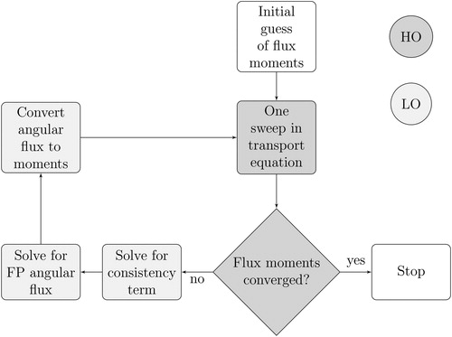
The main advantage of setting up the solver in this fashion is that the stiff matrix for LO needs to be setup and inverted only once, just as with FPSA (Patel et al. 2020; Patel 2016). This has a significant impact on the method’s performance. A flowchart of this algorithm is shown in Figure 1.

Figure 1. MFPA algorithm.

Naturally, Equations (2.11) can also be solved linearly. In that case, we can rewrite them using operator notation as follows: (2.13a) $$\mathcal{L}{\psi }_{HO}=\mathcal{S}{\psi }_{LO}+Q,$$(2.13a) (2.13b) $${\psi }_{LO}={\mathcal{P}}^{-1}\left(\mathcal{S}-\mathcal{F}-{\sigma }_{s,0}\mathcal{I}\right){\psi }_{HO}+{\mathcal{P}}^{-1}Q,$$(2.13b) where we substituted the definition of D_F into Equation (2.13b)(2.13b) $${\psi }_{LO}={\mathcal{P}}^{-1}\left(\mathcal{S}-\mathcal{F}-{\sigma }_{s,0}\mathcal{I}\right){\psi }_{HO}+{\mathcal{P}}^{-1}Q,$$(2.13b) . Substituting the definition of ψ_LO in Equation (2.13b)(2.13b) $${\psi }_{LO}={\mathcal{P}}^{-1}\left(\mathcal{S}-\mathcal{F}-{\sigma }_{s,0}\mathcal{I}\right){\psi }_{HO}+{\mathcal{P}}^{-1}Q,$$(2.13b) into Equation (2.13a)(2.13a) $$\mathcal{L}{\psi }_{HO}=\mathcal{S}{\psi }_{LO}+Q,$$(2.13a) and rearranging, we obtain (2.14) $${\psi }_{HO}={\left(\mathcal{I}-{\mathcal{L}}^{-1}\mathcal{S}{\mathcal{P}}^{-1}\mathcal{B}\right)}^{-1}\left[{\mathcal{L}}^{-1}\left(\mathcal{S}{\mathcal{P}}^{-1}+\mathcal{I}\right)Q\right],$$(2.14) where $\mathcal{B}=\mathcal{S}-\mathcal{F}-{\sigma }_{s,0}\mathcal{I}.$ Equation (2.14)(2.14) $${\psi }_{HO}={\left(\mathcal{I}-{\mathcal{L}}^{-1}\mathcal{S}{\mathcal{P}}^{-1}\mathcal{B}\right)}^{-1}\left[{\mathcal{L}}^{-1}\left(\mathcal{S}{\mathcal{P}}^{-1}+\mathcal{I}\right)Q\right],$$(2.14) can be solved using any linear solution technique, such as GMRES.

Due to the instability generated by having a zero value for the angular flux in the denominator of D for beam problems, the solutions obtained with the nonlinear term $D\psi$ fail to converge to the correct result. Bearing that in mind, from this point forward we only use the consistency term D_F in this paper.

3. Numerical experiments

In Section 3.1 we describe the discretization methods used to implement the algorithms. In Section 3.2 we provide numerical results for two different choices of source $\mathsf{Q}$ and boundary conditions. For each choice we solve the problem for homogeneous and heterogeneous slabs, and use three different scattering kernels, applying three different choices of parameters for each kernel. We provide MFPA numerical results for these cases and compare them against those obtained from FPSA and other methods.

All numerical experiments were performed using MATLAB. Runtime was tracked using the tic-toc functionality (MATLAB 2017), with only the solver runtime being taken into consideration in the comparisons. A 2017 MacBook Pro with a 2.8 GHz Quad-Core Intel Core i7 and 16 GB of RAM was used for all simulations.

3.1. Discretization

The transport and FP equations were discretized using linear discontinuous finite element discretization in space (Warsa and Prinja 2012), and discrete ordinates (S_N) in angle (Lewis and Miller 1993). The FP operator $\mathcal{F}$ was discretized using moment preserving discretization (MPD) (Warsa and Prinja 2012). Details of the derivation of the linear discontinuous finite element discretization can be seen in (Patel 2016; Martin 1976). The finite element discretization for the FP equation follows the same derivation.

A brief review for the angular discretization used for the FP equation is given below. First, we use Gauss-Legendre quadrature to discretize the FP equation in angle (Warsa and Prinja 2012): (3.15) $${\mu }_n\frac{\partial {\psi }_n(x)}{\partial x}+{\sigma }_a{\psi }_n(x)-\frac{{\sigma }_{tr}}{2}{\nabla }_n^2{\psi }_n(x)=Q_n(x),$$(3.15) for $n=1,..,N.$ Here, ${\nabla }_n^2=\frac{\partial }{\partial \mu }(1-{\mu }_n^2)\frac{\partial }{\partial \mu }$ is the discrete form of the angular Laplacian operator evaluated at angle n.

The MPD scheme is then shown as (Warsa and Prinja 2012) (3.16) $${\nabla }_n^2{\psi }_n=M{\psi }_n=V^{-1}LV{\psi }_n,$$(3.16) where M is the MPD discretized operator defined by (3.17a) $$V_{i,j}=P_{i-1}({\mu }_j)w_j$$(3.17a) and (3.17b) $$L_{i,j}=-i(i-1),$$(3.17b) for $i,j=1,\dots ,N.$ Here, $P_i({\mu }_j)$ are the Legendre polynomials evaluated at each angle μ_j and w_j are their respective weights. M is defined as a (N × N) operator for a vector of N angular fluxes $\psi (x)$ at spatial location x.

In summary, if we write the FP equation as (3.18) $$\mathcal{H}\frac{\partial \psi }{\partial x}(x)+{\sigma }_a\psi (x)-\mathcal{F}\psi (x)=\mathsf{Q}(x),$$(3.18) then $\mathcal{H}$ is Diag$({\mu }_n)$ for $n=1,\dots ,N,$ $\mathsf{Q}$(x) is a vector of source terms $Q_n(x),$ and $\mathcal{F}$ is represented by $\frac{{\sigma }_{tr}}{2}M.$

3.2. Numerical results

False convergence has been shown to result in inaccurate solutions for slowly converging problems (Adams and Larsen 2002). To work around this issue, the convergence criterion is modified to use information about the current and previous iteration: (3.19) $$\frac{\left|\right|{\varphi }_0^m(x)-{\varphi }_0^{m-1}(x)|{|}_2}{1-\frac{\left|\right|{\varphi }_0^{m+1}(x)-{\varphi }_0^m(x)|{|}_2}{\left|\right|{\varphi }_0^m(x)-{\varphi }_0^{m-1}(x)|{|}_2}}<{10}^{-8}.$$(3.19)

We simulated homogeneous and heterogeneous slab problems using 200 spatial cells, X = 400, ${\sigma }_a=0,$ L = 15, and N = 16. Problem set 1 has vacuum boundaries and a homogeneous, isotropic source $\mathsf{Q}$ for $0<x<X.$ Problem set 2 has no internal source and an incoming beam at the left boundary. The source and boundary conditions used are shown in Table 1.

Table 1. Problem parameters.

	Problem set 1	Problem set 2
Q(x)	0.5	0
ψL	0	$\delta (\mu -{\mu }_N)$
ψR	0	0

We consider three scattering kernels in this paper: Screened Rutherford (Pomraning 1992), Exponential (Pomraning et al. 1992), and Henyey–Greenstein (Henyey and Greenstein 1941). Three cases for each kernel were tested. The results obtained with MFPA using Picard iteration are compared with those obtained using S_N with DSA and FPSA with the MPD scheme.

Furthermore, results are also given for MFPA and FPSA using GMRES and compared with the results from MFPA using Picard iteration. MATLAB has a GMRES function (MATLAB, 2017) with built-in convergence criterion. The convergence criterion used for Picard iteration was chosen to match MATLAB’s GMRES function such that: (3.20) $$\frac{\left|\right|Q-(\mathcal{L}-S){\psi }_{HO}|{|}_2}{\left|\right|Q|{|}_2}<{10}^{-8}.$$(3.20)

3.2.1. SRK: screened Rutherford Kernel

The Screened Rutherford Kernel (Patel et al. 2020; Pomraning 1992) is a widely used scattering kernel for modeling scattering behavior of electrons (Dixon et al. 2015). The kernel depends on the screening parameter η (Dixon et al. 2015), such that (3.21) $${\sigma }_{s,l}^{\mathit{SRK}}={\sigma }_s{\int }_{-1}^{1}d\mu P_l(\mu )\frac{\eta (\eta +1)}{{(1+2\eta -\mu )}^2}.$$(3.21)

The SRK has a valid FP limit as η approaches 0 (Patel et al. 2020). Three different values of η were used to generate the scattering kernels shown in Figure 2. GMRES, DSA, FPSA, and MFPA all converged to the same solution for both problem sets. Figure 3 shows the solutions for SRK with $\eta ={10}^{-7}.$

Figure 2. Screened Rutherford Kernels.

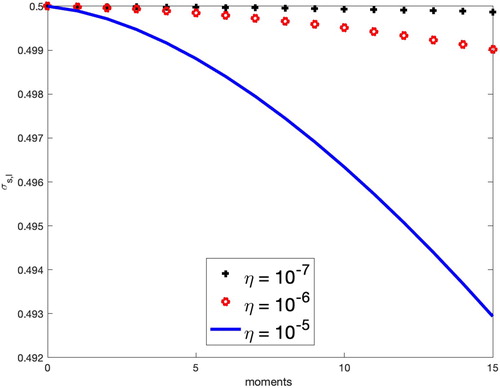
Figure 3. Results for SRK problems with $\eta ={10}^{-7}.$

Runtime and iteration count are shown Tables 2 and 3. We see that MFPA and FPSA have comparable results, both tremendously outperforming DSA in runtime for all cases. We see a reduction in runtime and iterations for FPSA and MFPA as the FP limit is approached, with DSA requiring many more iterations by comparison as η approaches 0.

Table 2. Runtime and iteration counts for Problem 1 with SRK.

Parameter	Solver	Runtime (s)	Iterations
$\eta ={10}^{-5}$	DSA	2380	53,585
	FPSA	1.21	26
	MFPA	1.39	26
$\eta ={10}^{-6}$	DSA	3040	69,156
	FPSA	0.747	16
	MFPA	0.857	16
$\eta ={10}^{-7}$	DSA	3270	73,940
	FPSA	0.475	10
	MFPA	0.542	10

Table 3. Runtime and iteration counts for Problem 2 with SRK.

Parameter	Solver	Runtime (s)	Iterations
$\eta ={10}^{-5}$	DSA	1107	25,072
	FPSA	0.953	20
	MFPA	1.14	20
$\eta ={10}^{-6}$	DSA	1434	32,562
	FPSA	0.730	14
	MFPA	0.857	14
$\eta ={10}^{-7}$	DSA	1470	33,246
	FPSA	0.438	8
	MFPA	0.484	8

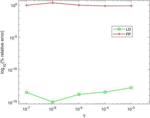
An advantage that MFPA offers is that the moments of angular flux in the LO equation will remain consistent with those of the transport equation even as a problem becomes less forward-peaked. On the other hand, the moments found using only the FP equation and source iteration lose accuracy. To illustrate this, Problem 1 was tested using different Screened Rutherford Kernels with increasing η parameters. The percent errors (relative to the transport solution) for the scalar flux obtained with the modified LO equation and with the standard FP equation at the center of the slab are shown in Figure 4. It can be seen that the percent relative errors in the scalar flux of the FP solution is orders of magnitude larger than the error produced using the LO equation. The same trend can be seen when using the exponential and Henyey–Greenstein kernels.

Figure 4. Log scale of % relative error vs. η for Problem 1 at the center of the slab with SRK.

In Tables 4 and 5, we provide a comparison of MFPA with Picard iteration against MFPA, FPSA, and non accelerated transport using GMRES. Here, the convergence criterion for MFPA-Picard was changed to match that of the MATLAB GMRES function shown in Equation (3.20)(3.20) $$\frac{\left|\right|Q-(\mathcal{L}-S){\psi }_{HO}|{|}_2}{\left|\right|Q|{|}_2}<{10}^{-8}.$$(3.20) .

Table 4. Runtime and iteration counts for Problem 1 with SRK.

Parameter	Solver	Runtime (s)	Iterations
$\eta ={10}^{-5}$	GMRES	143	2210
	FPSA-GMRES	0.589	11
	MFPA-Picard	1.02	18
	MFPA-GMRES	0.539	11
$\eta ={10}^{-6}$	GMRES	216	3780
	FPSA-GMRES	0.367	6
	MFPA-Picard	0.558	10
	MFPA-GMRES	0.399	7
$\eta ={10}^{-7}$	GMRES	168	3600
	FPSA-GMRES	0.274	6
	MFPA-Picard	0.301	5
	MFPA-GMRES	0.311	4

Table 5. Runtime and iteration counts for Problem 2 with SRK.

Parameter	Solver	Runtime (s)	Iterations
$\eta ={10}^{-5}$	GMRES	62.6	810
	FPSA-GMRES	0.608	11
	MFPA-Picard	0.664	12
	MFPA-GMRES	0.517	10
$\eta ={10}^{-6}$	GMRES	107	72
	FPSA-GMRES	0.432	7
	MFPA-Picard	0.347	6
	MFPA-GMRES	0.389	7
$\eta ={10}^{-7}$	GMRES	113	1458
	FPSA-GMRES	0.309	4
	MFPA-Picard	0.237	4
	MFPA-GMRES	0.357	4

We see that FPSA-GMRES, MFPA-Picard, and MFPA-GMRES drastically outperform GMRES in runtime and iterations. FPSA-GMRES and MFPA-GMRES have faster runtimes for most of the SRK problems tested. However, it is important to keep in mind that the setup time for all methods is not taken into account in these results. Setting up the preconditioners in FPSA-GMRES and MFPA-GMRES takes additional time. We note that MFPA-Picard is the fastest method overall.

3.2.2. EK: exponential kernel

The exponential kernel (Patel et al. 2020; Pomraning et al. 1992) is a fictitious kernel made for problems that have a valid Fokker–Planck limit (Pomraning 1992). The zero${}^{\text{th}}$ moment, ${\sigma }_{s,0}^{EK},$ is chosen arbitrarily; we define ${\sigma }_{s,0}^{EK}$ as the same zero${}^{\text{th}}$ moment from the SRK. The Δ parameter determines the kernel: the first and second moments are given by (3.22a) $${\sigma }_{s,1}^{EK}={\sigma }_{s,0}^{EK}(1-\Delta ),$$(3.22a) (3.22b) $${\sigma }_{s,2}^{EK}={\sigma }_{s,0}^{EK}(1-3\Delta +3{\Delta }^2),$$(3.22b) and the relationship for $l\ge 3$ is (3.22c) $${\sigma }_{s,l+1}^{EK}={\sigma }_{s,l-1}^{EK}-\Delta (2l+1){\sigma }_{s,l}^{EK}.$$(3.22c)

As Δ is reduced, the scattering kernel becomes more forward-peaked.

The EK has a valid FP limit (Patel et al. 2020). Three different values of Δ were used to generate the scattering kernels shown in Figure 5. GMRES, DSA, FPSA, and MFPA all converged to the same solution for problem sets 1 and 2. Figure 6 shows the solutions for EK with $\Delta ={10}^{-7}.$

Figure 5. Exponential Kernels.

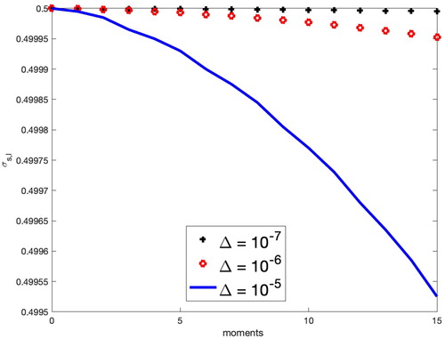
Figure 6. Results for EK Problems with $\Delta ={10}^{-7}.$

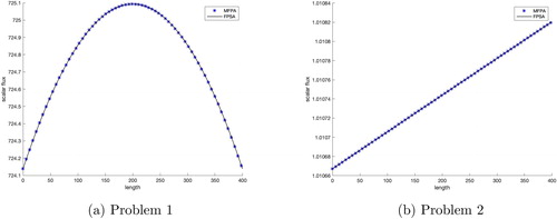
The runtimes and iterations for DSA, FPSA, and MFPA are shown in Tables 6 and 7. We see a similar trend with the EK as seen with SRK, in that smaller Δ values lead to a reduction in runtime and iterations for MFPA and FPSA, which greatly outperform DSA in both categories.

Table 6. Runtime and iteration counts for Problem 1 with EK.

Parameter	Solver	Runtime (s)	Iterations
$\Delta ={10}^{-5}$	DSA	3110	70,140
	FPSA	0.514	11
	MFPA	0.630	11
$\Delta ={10}^{-6}$	DSA	3120	70,758
	FPSA	0.388	7
	MFPA	0.393	7
$\Delta ={10}^{-7}$	DSA	3120	70,851
	FPSA	0.292	6
	MFPA	0.318	6

Table 7. Runtime and iteration counts for Problem 2 with EK.

Parameter	Solver	Runtime (s)	Iterations
$\Delta ={10}^{-5}$	DSA	1455	33,033
	FPSA	0.492	10
	MFPA	0.613	10
$\Delta ={10}^{-6}$	DSA	1470	33,309
	FPSA	0.358	7
	MFPA	0.431	7
$\Delta ={10}^{-7}$	DSA	1470	33,339
	FPSA	0.273	5
	MFPA	0.319	5

The comparison of runtimes and iterations of non accelerated transport, MFPA, and FPSA using GMRES against MFPA using Picard iteration with the updated convergence criterion for the Exponential Kernel are given in Tables 8 and 9.

Table 8. Runtime and iteration counts for Problem 1 with EK.

Parameter	Solver	Runtime (s)	Iterations
$\Delta ={10}^{-5}$	GMRES	206	4140
	FPSA-GMRES	0.320	5
	MFPA-Picard	0.350	6
	MFPA-GMRES	0.298	5
$\Delta ={10}^{-6}$	GMRES	143	2860
	FPSA-GMRES	0.237	3
	MFPA-Picard	0.240	4
	MFPA-GMRES	0.228	3
$\Delta ={10}^{-7}$	GMRES	124	486
	FPSA-GMRES	0.228	3
	MFPA-Picard	0.185	3
	MFPA-GMRES	0.226	3

Table 9. Runtime and iteration counts for Problem 2 with EK.

Parameter	Solver	Runtime (s)	Iterations
$\Delta ={10}^{-5}$	GMRES	96.0	544
	FPSA-GMRES	0.324	5
	MFPA-Picard	0.257	4
	MFPA-GMRES	0.293	5
$\Delta ={10}^{-6}$	GMRES	80.1	533
	FPSA-GMRES	0.236	3
	MFPA-Picard	0.183	3
	MFPA-GMRES	0.226	3
$\Delta ={10}^{-7}$	GMRES	62.8	1110
	FPSA-GMRES	0.237	3
	MFPA-Picard	0.126	2
	MFPA-GMRES	0.182	2

We see a similar behavior to the SRK problems for runtimes and iterations of MFPA-Picard when compared to FPSA-GMRES, MFPA-GMRES, and non accelerated GMRES. Once again, we note that FPSA-GMRES and MFPA-GMRES require extra time for the setup of the preconditioner, adding more time to the results shown in the tables.

3.2.3. HGK: Henyey–Greenstein Kernel

The Henyey–Greenstein Kernel (Henyey and Greenstein 1941; Patel et al. 2020) is most commonly used in light transport in clouds. It relies on the anisotropy factor g, such that (3.23) $${\sigma }_{s,l}^{\mathit{HGK}}={\sigma }_s{g}^l.$$(3.23)

As g goes from zero to unity, the scattering shifts from isotropic to highly anisotropic.

The HGK does not have a valid FP limit (Patel et al. 2020). The three kernels tested are shown in Figure 7. GMRES, DSA, FPSA, and MFPA all converged to the same solution for problem sets 1 and 2. Figure 8 shows the solutions for HGK with g = 0.99. The results of each solver are shown in Tables 10 and 11.

Figure 7. Henyey–Greenstein Kernels.

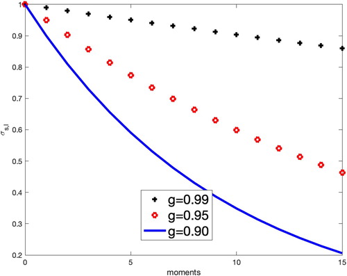
Figure 8. Results for HGK Problems with g = 0.99.

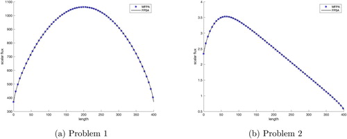
Table 10. Runtime and iteration counts for Problem 1 with HGK.

Parameter	Solver	Runtime (s)	Iterations
g = 0.9	DSA	24.5	554
	FPSA	1.50	32
	MFPA	1.39	27
g = 0.95	DSA	47.7	1083
	FPSA	1.75	38
	MFPA	1.83	35
g = 0.99	DSA	243	5530
	FPSA	3.38	74
	MFPA	3.93	73

Table 11. Runtime and iteration counts for Problem 2 with HGK.

Parameter	Solver	Runtime (s)	Iterations
g = 0.9	DSA	14.8	336
	FPSA	1.15	23
	MFPA	1.35	24
g = 0.95	DSA	29.7	675
	FPSA	1.56	32
	MFPA	1.90	33
g = 0.99	DSA	146	3345
	FPSA	3.31	67
	MFPA	3.99	67

Here we see that MFPA and FPSA do not perform as well compared to their results for the SRK and EK. Contrary to what happened in those cases, both solvers require more time and iterations as the problem becomes more anisotropic. This is somewhat expected, due to HGK not having a valid Fokker–Planck limit. However, both MFPA and FPSA continue to greatly outperform DSA.

Once again, we compare runtimes and iterations of non accelerated transport, MFPA, and FPSA using GMRES against MFPA using Picard iteration with the updated convergence criterion, given in Tables 12 and 13.

Table 12. Runtime and iteration counts for Problem 1 with HGK.

Parameter	Solver	Runtime (s)	Iterations
g = 0.9	GMRES	98.6	92
	FPSA-GMRES	0.494	9
	MFPA-Picard	1.24	21
	MFPA-GMRES	0.512	10
g = 0.95	GMRES	106	2112
	FPSA-GMRES	0.618	12
	MFPA-Picard	1.63	29
	MFPA-GMRES	0.632	13
g = 0.99	GMRES	85.7	1131
	FPSA-GMRES	1.161	24
	MFPA-Picard	3.13	58
	MFPA-GMRES	1.135	26

Table 13. Runtime and iteration counts for Problem 2 with HGK.

Parameter	Solver	Runtime (s)	Iterations
g = 0.9	GMRES	29.1	265
	FPSA-GMRES	0.678	13
	MFPA-Picard	1.07	19
	MFPA-GMRES	0.659	14
g = 0.95	GMRES	36.9	330
	FPSA-GMRES	0.864	17
	MFPA-Picard	1.46	26
	MFPA-GMRES	0.863	19
g = 0.99	GMRES	39.9	14
	FPSA-GMRES	1.53	32
	MFPA-Picard	2.98	54
	MFPA-GMRES	1.49	35

HGK presents a similar trend compared to SRK and EK. FPSA-GMRES, MFPA-Picard, MFPA-GMRES all outperform non accelerated GMRES.

3.2.4. Heterogeneous problems

In order to test the accuracy of the method when dealing with interface conditions, we tested two heterogeneous slab problems. We use the same general parameters as in the previous sections, with the modification of 100 spatial cells, X = 100, and ${\sigma }_a=0.0001.$ We setup the heterogeneous slab similar to the one in Pomraning (2000), with a step function cross section given by (3.24) $${\overline{\sigma }}_{s,0}(x)=\{\begin{array}{cc}{\sigma }_{s,0}(x)(1+ϵ),\hfill & 0\le x\le \frac{X}{2}\hfill \\ {\sigma }_{s,0}(x)(1-ϵ),\hfill & \frac{X}{2}\le x\le X\hfill \end{array}$$(3.24) where ϵ is a constant. We consider the SRK with ${\sigma }_{s,0}=0.5$ and $\eta ={10}^{-7},$ the EK with ${\sigma }_{s,0}=0.5$ and $\Delta ={10}^{-7},$ and the HGK with ${\sigma }_{s,0}=1.0$ and g = 0.99. The values of ϵ are chosen as −0.8, –0.4, 0.4, 0.8. We tested non accelerated GMRES and MFPA using finite element discretization and Picard iteration with the convergence criterion shown in Equation (3.20)(3.20) $$\frac{\left|\right|Q-(\mathcal{L}-S){\psi }_{HO}|{|}_2}{\left|\right|Q|{|}_2}<{10}^{-8}.$$(3.20) .

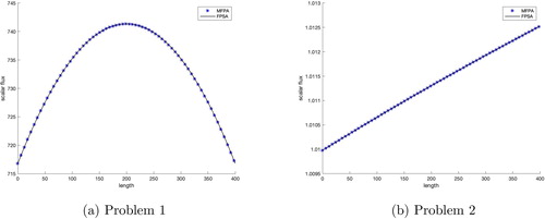
Figures 9 and 10 show the SRK results for the heterogeneous slab problems tested. GMRES and MFPA converged to the same result. We expect to see a reflective relationship due to our choice of ϵ and definition of the cross section as a step function. MFPA showed no loss of accuracy in heterogeneous media using the SRK.

Figure 9. Results for heterogeneous Problem 1 using SRK with $ϵ=\pm 0.4,\pm 0.8.$

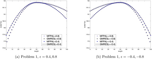
Figure 10. Results for heterogeneous Problem 2 using SRK with $ϵ=\pm 0.4,\pm 0.8.$

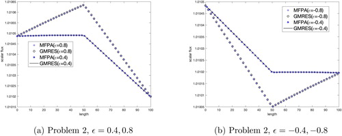
Figure 11. Results for heterogeneous Problem 1 using EK with $ϵ=\pm 0.4,\pm 0.8.$

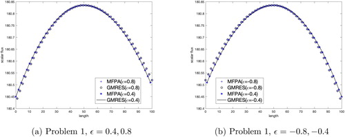
Figure 12. Results for heterogeneous Problem 2 using EK with $ϵ=\pm 0.4,\pm 0.8.$

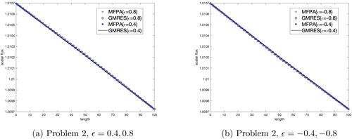
Figure 13. Results for heterogeneous Problem 1 using HGK with $ϵ=\pm 0.4,\pm 0.8.$

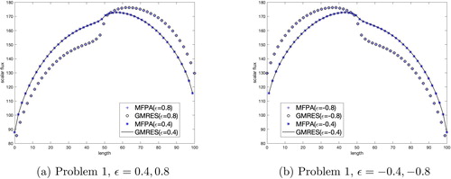
Figure 14. Results for heterogeneous Problem 2 using HGK with $ϵ=\pm 0.4,\pm 0.8.$

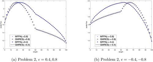
We see similar results in Figures 11 and 12 when testing the EK in the heterogeneous slab problems. The changes in scalar flux are not as significant as in the SRK when using the step function cross section. The accuracy of the MFPA method in this heterogeneous slab has not been negatively affected.

We see interesting results in Figures 13 and 14 when testing the HGK in the heterogeneous slab problems. Once again, MFPA and GMRES converged to the same solution, with MFPA having no loss of accuracy in the heterogeneous slab.

4. Angularly-discrete Fourier analysis for MFPA

In this section we analyze MFPA using angular-discrete Fourier analysis. Our goal is to theoretically determine how efficient the proposed method is through the spectral radius of the iteration matrix. This analysis closely follows the work done in Patel et al. (2020).

We begin with rewriting Equations (2.11(2.11a) $$\text{HO}:\mu \frac{\partial {\psi }_{HO}}{\partial x}+{\sigma }_t{\psi }_{HO}=\sum _{l=0}^L\frac{(2l+1)}{2}{P}_l{\sigma }_{s,l}{\varphi }_{l,LO}+Q ,$$(2.11a) ) using source iteration, as (4.1a) $$\mu \frac{\partial {\psi }_{HO}^{k+1}}{\partial x}+{\sigma }_t{\psi }_{HO}^{k+1}=\sum _{l=0}^L\frac{(2l+1)}{2}{P}_l{\sigma }_{s,l}{\varphi }_{l,LO}^{k+1}+Q ,$$(4.1a) (4.1b) $$\begin{array}{c}\mu \frac{\partial {\psi }_{LO}^{k+1}}{\partial x}+{\sigma }_a{\psi }_{LO}^{k+1}-\frac{{\sigma }_{tr}}{2}\frac{\partial }{\partial \mu }(1-{\mu }^2)\frac{\partial {\psi }_{LO}^{k+1}}{\partial \mu }=\hfill \\ \mathrm{\hspace{1em}}\mathrm{\hspace{1em}}Q+\sum _{l=0}^L\frac{(2l+1)}{2}{P}_l{\sigma }_{s,l}{\varphi }_{l,HO}^k-\frac{{\sigma }_{tr}}{2}\frac{\partial }{\partial \mu }(1-{\mu }^2)\frac{\partial {\psi }_{HO}^k}{\partial \mu }-{\sigma }_{s,0}{\psi }_{HO}^k .\hfill \end{array}$$(4.1b)

Subtracting the exact Equations (2.11a)(2.11a) $$\text{HO}:\mu \frac{\partial {\psi }_{HO}}{\partial x}+{\sigma }_t{\psi }_{HO}=\sum _{l=0}^L\frac{(2l+1)}{2}{P}_l{\sigma }_{s,l}{\varphi }_{l,LO}+Q ,$$(2.11a) and (2.11b)(2.11b) $$\text{LO}:\mu \frac{\partial {\psi }_{LO}}{\partial x}+{\sigma }_a{\psi }_{LO}=\frac{{\sigma }_{tr}}{2}\frac{\partial }{\partial \mu }(1-{\mu }^2)\frac{\partial {\psi }_{LO}}{\partial \mu }+D_F+Q ,$$(2.11b) from Equations (4.1(4.1a) $$\mu \frac{\partial {\psi }_{HO}^{k+1}}{\partial x}+{\sigma }_t{\psi }_{HO}^{k+1}=\sum _{l=0}^L\frac{(2l+1)}{2}{P}_l{\sigma }_{s,l}{\varphi }_{l,LO}^{k+1}+Q ,$$(4.1a) ) returns the error equations (4.2a) $$\mu \frac{\partial {ϵ}_{HO}^{k+1}}{\partial x}+{\sigma }_t{ϵ}_{HO}^{k+1}=\sum _{l=0}^L\frac{(2l+1)}{2}{P}_l{\sigma }_{s,l}{ϵ}_{LO}^{k+1} ,$$(4.2a) (4.2b) $$\begin{array}{c}\mu \frac{\partial {ϵ}_{LO}^{k+1}}{\partial x}+{\sigma }_a{ϵ}_{LO}^{k+1}-\frac{{\sigma }_{tr}}{2}\frac{\partial }{\partial \mu }(1-{\mu }^2)\frac{\partial {ϵ}_{LO}^{k+1}}{\partial \mu }=\hfill \\ \mathrm{\hspace{1em}}\mathrm{\hspace{1em}}\sum _{l=0}^L\frac{(2l+1)}{2}{P}_l{\sigma }_{s,l}{ϵ}_{HO}^k-\frac{{\sigma }_{tr}}{2}\frac{\partial }{\partial \mu }(1-{\mu }^2)\frac{\partial {ϵ}_{HO}^k}{\partial \mu }-{\sigma }_{s,0}{ϵ}_{HO}^k ,\hfill \end{array}$$(4.2b) where the error in the HO and LO angular flux are defined as (4.3a) $${\widehat{ϵ}}_{HO}^{k+1}={\psi }_{HO}^{k+1}-{\psi }_{HO},$$(4.3a) (4.3b) $${\widehat{ϵ}}_{HO}^k={\psi }_{HO}^k-{\psi }_{HO},$$(4.3b) (4.3c) $${\widehat{ϵ}}_{LO}^{k+1}={\psi }_{LO}^{k+1}-{\psi }_{LO}.$$(4.3c)

To perform Fourier analysis, we introduce the following Fourier mode ansatz for the HO and LO errors: (4.4a) $${\widehat{ϵ}}_{HO}^{k+1}={ϵ}_{HO}^{k+1}(\mu )e^{i{\sigma }_t\lambda x},$$(4.4a) (4.4b) $${\widehat{ϵ}}_{HO}^k={ϵ}_{HO}^k(\mu )e^{i{\sigma }_t\lambda x},$$(4.4b) (4.4c) $${\widehat{ϵ}}_{LO}^{k+1}={ϵ}_{LO}^{k+1}(\mu )e^{i{\sigma }_t\lambda x}.$$(4.4c)

Substituting Equations (4.4a)(4.4a) $${\widehat{ϵ}}_{HO}^{k+1}={ϵ}_{HO}^{k+1}(\mu )e^{i{\sigma }_t\lambda x},$$(4.4a) and (4.4c)(4.4c) $${\widehat{ϵ}}_{LO}^{k+1}={ϵ}_{LO}^{k+1}(\mu )e^{i{\sigma }_t\lambda x}.$$(4.4c) into Equation (4.2a)(4.2a) $$\mu \frac{\partial {ϵ}_{HO}^{k+1}}{\partial x}+{\sigma }_t{ϵ}_{HO}^{k+1}=\sum _{l=0}^L\frac{(2l+1)}{2}{P}_l{\sigma }_{s,l}{ϵ}_{LO}^{k+1} ,$$(4.2a) and simplifying, leads to (4.5) $$\left({\sigma }_t+i{\sigma }_t\lambda \mu \right){ϵ}_{HO}^{k+1}=\sum _{l=0}^L\frac{(2l+1)}{2}{P}_l{\sigma }_{s,l}{ϵ}_{LO}^{k+1}$$(4.5)

Next, we take the $n^{\text{th}}$ Legendre moment of Equation (4.5)(4.5) $$\left({\sigma }_t+i{\sigma }_t\lambda \mu \right){ϵ}_{HO}^{k+1}=\sum _{l=0}^L\frac{(2l+1)}{2}{P}_l{\sigma }_{s,l}{ϵ}_{LO}^{k+1}$$(4.5) and use the orthogonality property of Legendre polynomials, which allows us to write (4.6) $$\underset{-1}{\overset{1}{\int }}d\mu P_l(\mu )\left({\sigma }_t+i{\sigma }_t\lambda \mu \right){ϵ}_{HO}^{k+1}=\underset{-1}{\overset{1}{\int }}d\mu P_l(\mu ){\sigma }_{s,l}{ϵ}_{l,LO}^{k+1},$$(4.6) where ${ϵ}_{l,LO}^{k+1}$ represents the LO flux moment error. Here, the flux moment error is defined as (4.7) $${ϵ}_l^k={\int }_{-1}^{1}d\mu P_l(\mu ){ϵ}^k=\sum _{n=1}^N{w}_n{P}_l({\mu }_n){ϵ}^k .$$(4.7)

We can now rewrite the integrals as weighted sums: (4.8) $$\underset{Y}{\underbrace{\sum _{n=1}^N{P}_l({\mu }_n)w_n\left({\sigma }_t+i{\sigma }_t\lambda {\mu }_n\right)}}{ϵ}_{HO}^{k+1}=\underset{Z}{\underbrace{\sum _{n=1}^N{P}_l({\mu }_n)w_n{\sigma }_{s,l}}}{ϵ}_{LO}^{k+1},$$(4.8) and further simplify this equation to get the HO matrix equation (4.9) $${ϵ}_{HO}^{k+1}=\underset{\widehat{A}}{\underbrace{Y^{-1}Z}}{ϵ}_{LO}^{k+1}.$$(4.9)

Here, $\widehat{A}$ is part of the MFPA iteration matrix.

Similarly, substituting Equations (4.4b)(4.4b) $${\widehat{ϵ}}_{HO}^k={ϵ}_{HO}^k(\mu )e^{i{\sigma }_t\lambda x},$$(4.4b) and (4.4c)(4.4c) $${\widehat{ϵ}}_{LO}^{k+1}={ϵ}_{LO}^{k+1}(\mu )e^{i{\sigma }_t\lambda x}.$$(4.4c) into Equations (4.2b)(4.2b) $$\begin{array}{c}\mu \frac{\partial {ϵ}_{LO}^{k+1}}{\partial x}+{\sigma }_a{ϵ}_{LO}^{k+1}-\frac{{\sigma }_{tr}}{2}\frac{\partial }{\partial \mu }(1-{\mu }^2)\frac{\partial {ϵ}_{LO}^{k+1}}{\partial \mu }=\hfill \\ \mathrm{\hspace{1em}}\mathrm{\hspace{1em}}\sum _{l=0}^L\frac{(2l+1)}{2}{P}_l{\sigma }_{s,l}{ϵ}_{HO}^k-\frac{{\sigma }_{tr}}{2}\frac{\partial }{\partial \mu }(1-{\mu }^2)\frac{\partial {ϵ}_{HO}^k}{\partial \mu }-{\sigma }_{s,0}{ϵ}_{HO}^k ,\hfill \end{array}$$(4.2b) and simplifying returns (4.10) $$\begin{array}{l}\left(i{\sigma }_t\lambda \mu +{\sigma }_a-\frac{{\sigma }_{tr}}{2}\frac{\partial }{\partial \mu }(1-{\mu }^2)\frac{\partial }{\partial \mu }\right){ϵ}_{LO}^{k+1}=\hfill \\ \mathrm{\hspace{1em}}\mathrm{\hspace{1em}}\left(\sum _{l=0}^L\frac{(2l+1)}{2}{P}_l{\sigma }_{s,l}-\frac{{\sigma }_{tr}}{2}\frac{\partial }{\partial \mu }(1-{\mu }^2)\frac{\partial }{\partial \mu }-{\sigma }_{s,0}\right){ϵ}_{HO}^k .\hfill \end{array}$$(4.10)

Now, we operate on Equation (4.10)(4.10) $$\begin{array}{l}\left(i{\sigma }_t\lambda \mu +{\sigma }_a-\frac{{\sigma }_{tr}}{2}\frac{\partial }{\partial \mu }(1-{\mu }^2)\frac{\partial }{\partial \mu }\right){ϵ}_{LO}^{k+1}=\hfill \\ \mathrm{\hspace{1em}}\mathrm{\hspace{1em}}\left(\sum _{l=0}^L\frac{(2l+1)}{2}{P}_l{\sigma }_{s,l}-\frac{{\sigma }_{tr}}{2}\frac{\partial }{\partial \mu }(1-{\mu }^2)\frac{\partial }{\partial \mu }-{\sigma }_{s,0}\right){ϵ}_{HO}^k .\hfill \end{array}$$(4.10) by ${\int }_{-1}^{1}d\mu P_l(\mu ),$ rewrite the integrals as weighted sums, and use moment preserving discretization (MPD) (Warsa and Prinja 2012) for the Fokker–Planck in-scattering term $\frac{\partial }{\partial \mu }(1-{\mu }^2)\frac{\partial }{\partial \mu }.$ This yields the LO matrix equation (4.11) $$\begin{array}{c}\underset{\widehat{B}}{\underbrace{\sum _{n=1}^N{P}_l({\mu }_n)w_n\left(i{\sigma }_t\lambda \mu +{\sigma }_a+\frac{{\sigma }_{tr}}{2}l(l+1)\right)}}{ϵ}_{LO}^{k+1}\hfill \\ =\underset{\widehat{C}}{\underbrace{\sum _{n=1}^N{P}_l({\mu }_n)w_n\left({\sigma }_{s,l}-{\sigma }_{s,0}-\frac{{\sigma }_{tr}}{2}l(l+1)\right)}}{ϵ}_{HO}^k.\hfill \end{array}$$(4.11)

Finally, we combine Equations (4.9)(4.9) $${ϵ}_{HO}^{k+1}=\underset{\widehat{A}}{\underbrace{Y^{-1}Z}}{ϵ}_{LO}^{k+1}.$$(4.9) and (4.11)(4.11) $$\begin{array}{c}\underset{\widehat{B}}{\underbrace{\sum _{n=1}^N{P}_l({\mu }_n)w_n\left(i{\sigma }_t\lambda \mu +{\sigma }_a+\frac{{\sigma }_{tr}}{2}l(l+1)\right)}}{ϵ}_{LO}^{k+1}\hfill \\ =\underset{\widehat{C}}{\underbrace{\sum _{n=1}^N{P}_l({\mu }_n)w_n\left({\sigma }_{s,l}-{\sigma }_{s,0}-\frac{{\sigma }_{tr}}{2}l(l+1)\right)}}{ϵ}_{HO}^k.\hfill \end{array}$$(4.11) to obtain the final matrix equation (4.12) $${ϵ}_{HO}^{k+1}=\widehat{A}{\widehat{B}}^{-1}\widehat{C}{ϵ}_{HO}^k,$$(4.12) where $\widehat{A}{\widehat{B}}^{-1}\widehat{C}$ is the iteration matrix, such that its spectral radius determines the convergence rate of MFPA with MPD.

Next, we test the results of this analysis against our numerical results. The theoretical spectral radius (ρ_th) was tested using ${\sigma }_a=0.0001{\sigma }_{s,0},$ L = 15, and N = 16. The numerical spectral radius (ρ_nu) was tested for a homogeneous slab with vacuum boundaries and an isotropic source Q = 0.5 for $0<x<X.$ We used 200 spatial cells, X = 400, ${\sigma }_a=0.0001{\sigma }_{s,0},$ L = 15, and N = 16. The 2-norm with a tolerance of ${10}^{-10}$ was used for convergence. Table 14 shows the results for ρ_th and ρ_nu.

Table 14. Theoretical spectral radius results for MFPA.

Kernel	Parameter	ρth	ρnu
SRK	$\eta ={10}^{-7}$	0.298	0.299
EK	$\Delta ={10}^{-7}$	0.114	0.110
HGK	g = 0.99	0.760	0.759

We observe that the numerical and theoretical spectral radii are in close agreement for all kernels. We also compare the MFPA theoretical spectral radius for each kernel with the theoretical spectral radius of source iteration and FPSA, as shown in Figure 15.

Figure 15. Results of ρ_th for SRK, EK, and HGK.

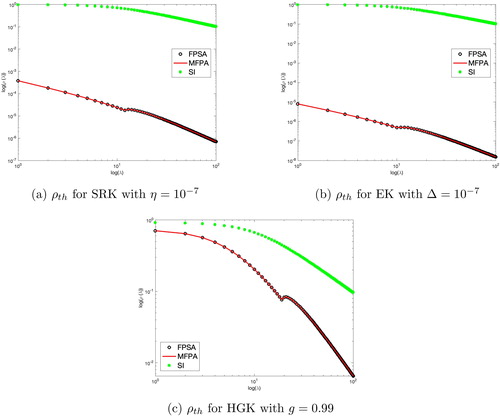
We see that the spectral radii of MFPA and FPSA are very close, which is expected due to the similarity of the methods. Both MFPA and FPSA have significantly smaller spectral radii compared to source iteration.

5. Discussion

This paper introduced the Modified FP Acceleration technique for steady-state, monoenergetic transport in slab geometry. Upon convergence, the modified FP and the transport models are consistent; in other words, the (lower order) modified FP equation preserves the moments of angular flux of the (higher order) transport equation.

MFPA was tested on both homogeneous and heterogeneous media with an isotropic internal source with vacuum boundaries, and with no internal source and an incoming beam in the left boundary. For both sets of problems, three different scattering kernels were used. The runtime and iterations of MFPA and FPSA were shown to be similar to each other, both vastly outperforming DSA for all cases by orders of magnitude. However, MFPA has the feature of preserving the moments of angular flux of the HO equation, which offers the advantage of integrating the LO model into multiphysics models.

MFPA, FPSA, and non accelerated transport using GMRES were compared to MFPA using Picard iteration. MFPA using both solvers and FPSA using GMRES notably outperformed non accelerated GMRES. Furthermore, although solver runtimes were similar for MFPA using both solvers and FPSA-GMRES, the setting up times of the preconditioners for the GMRES approaches were relatively large, making them slower overall than MFPA with Picard iteration.

Angularly-discrete Fourier analysis was performed on MFPA. The numerical and theoretical spectral radii were determined and found to be consistent. The MFPA theoretical spectral radii were compared with those of FPSA and source iteration.

In the future, we will investigate whether there is a formal mathematical relationship between FPSA and MFPA. We intend to test MFPA capabilities for a variety of multiphysics problems and analyze its performance. Moreover, we remark that in order to apply the proposed method to more realistic problems, it needs to be adapted to address geometries with higher order spatial dimensions. In future work, we will expand to more realistic problems as we continue to develop the method.

Acknowledgments

The authors would also like to thank Dr. James Warsa for his synthetic acceleration codes, and both Dr. Warsa and Dr. Anil Prinja for discussions involving Fokker–Planck acceleration. The statements, findings, conclusions, and recommendations are those of the authors and do not necessarily reflect the view of the U.S. Nuclear Regulatory Commission.

Additional information

Funding

The authors acknowledge support under award number NRC-HQ-84-15-G-0024 from the Nuclear Regulatory Commission.

References

- Adams, M. L., and E. W. Larsen. 2002. Fast iterative methods for discrete ordinates particle transport problems. Prog. Nucl. Energy 40 (1):3–159. doi:https://doi.org/10.1016/S0149-1970(01)00023-3
- Alcouffe, R. E. 1977. Diffusion synthetic acceleration for diamond-differenced discrete-ordinates equations. Nucl. Sci. Eng. 64 (2):344–55. doi:https://doi.org/10.13182/NSE77-1
- Aristova, E. N., and V. Y. Gol'din. 2000. Computation of anisotropy scattering of solar radiation in atmosphere (monoenergetic case). J. Quant. Spectrosc. Radiat. Transf. 67 (2):139–57. doi:https://doi.org/10.1016/S0022-4073(99)00201-0
- Carl, K. 2003. Solving Nonlinear Equations with Newton’s Method. Philadelphia: SIAM.
- Dixon, D. A., A. K. Prinja, and B. C. Franke. 2015. A computationally efficient moment-preserving Monte Carlo electron transport method with implementation in GEANT4. Ph.D. thesis, the University of New Mexico, Albuquerque. doi:https://doi.org/10.1016/j.nimb.2015.07.009
- Henyey, L. C., and J. L. Greenstein. 1941. Diffuse radiation in the galaxy. Astrophys. J. 93:70–83. doi:https://doi.org/10.1086/144246
- Khattab, K. M., and E. W. Larsen. 1991. Synthetic acceleration methods for linear transport problems with highly anisotropic scattering. Nucl. Sci. Eng. 107 (3):217–27. doi:https://doi.org/10.13182/NSE91-A23786
- Knoll, D. A., H. Park, and K. Smith. 2011. Application of the Jacobian-free Newton-Krylov method to nonlinear acceleration of transport source iteration in slab geometry. Nucl. Sci. Eng. 167 (2):122–32. doi:https://doi.org/10.13182/NSE09-75
- Lewis, E. E., and W. F. Miller, Jr. 1993. Computational methods of neutron transport. La Grange Park, IL: American Nuclear Society.
- Martin, W. R. 1976. The application of the finite element method to the neutron transport equation. Ph.D. thesis., The University of Michigan, Ann Arbor, MI.
- MATLAB, version 9.3.0.713579 (R2017b). 2017. The MathWorks Inc., Natick, Massachusetts.
- Patel, J. K. 2016. Fokker–Planck-based acceleration for SN equations with highly forward-peaked scattering in slab geometry. Ph.D. thesis., The University of New Mexico, Albuquerque, NM.
- Patel, J. K., H. Park, C. R. E. de Oliveira, and D. A. Knoll. 2014. Efficient multiphysics coupling for fast burst reactors in slab geometry. J. Comput. Theor. Transp. 43 (1–7):289–313. doi:https://doi.org/10.1080/00411450.2014.915222
- Patel, J. K., R. Vasques, and B. D. Ganapol. 2019. Towards a multiphyiscs model for tumor response to combined-hyperthermia-radiotherapy treatment. In Proceedings of International Conference on Mathematics & Computational Methods Applied to Nuclear Science & Engineering, Portland, OR, August 25–29.
- Patel, J. K., J. S. Warsa, and A. K. Prinja. 2020. Accelerating the solution of the SN equations with highly anisotropic scattering using the Fokker–Planck approximation. Ann. Nucl. Energy. 147:107665. doi:https://doi.org/10.1016/j.anucene.2020.107665
- Pomraning, G. C. 1992. The Fokker–Planck operator as an asymptotic limit. Math. Models Methods Appl. Sci. 2 (1):21–36. doi:https://doi.org/10.1142/S021820259200003X
- Pomraning, G. C. 2000. The screened Rutherford pencil beam problem with heterogeneities. Nucl. Sci. Eng. 136 (1):1–14. doi:https://doi.org/10.13182/NSE00-A2144
- Pomraning, G. C., A. K. Prinja, and J. W. VanDenburg. 1992. An asymptotic model for the spreading of a collimated beam. Nucl. Sci. Eng. 112 (4):347–60. doi:https://doi.org/10.13182/NSE92-A23983
- Saad, Y., and M. H. Schultz. 1986. GMRES: A generalized minimal residual algorithm for solving nonsymmetric linear systems. SIAM J. Sci. Stat. Comput. 7 (3):856–69. doi:https://doi.org/10.1137/0907058
- Turcksin, B., J. C. Ragusa, and J. E. Morel. 2012. Angular multigrid preconditioner for Krylov-based solution techniques applied to the Sn equations with highly forward-peaked scattering. Transp. Theory Stat. Phys. 41:1–22.
- Warsa, J. S., and A. K. Prinja. 2012. A moment preserving SN discretization for the one-dimensional Fokker–Planck equation. Trans. Am. Nucl. Soc. 106:362–5.