System-level operational cyber risks identification in industrial control systems

ABSTRACT

In Industrial Control Systems (ICS), where complex interdependencies abound, cyber incidents can have far-reaching consequences. Dependency modelling, a valuable technique for assessing cyber risks, aims to decipher relationships among variables. However, its effectiveness is often hampered by limited data exposure, hindering the analysis of direct and indirect impacts. We present a unique method that transforms dependency modelling data into a Bayesian Network (BN) structure and leverages causality and reasoning to extract inferences from seemingly unrelated events. Using operational ICS data, we confirm our method enables stakeholders to make better decisions about system security, stability, and reliability.

KEYWORDS:

• Industrial controls systems
• cyber risk
• dependency modelling
• Bayesian network

1. Introduction

The cyber security landscape in the Industrial Control Systems (ICS) continues to evolve rapidly, and it is vital for asset owners to adapt their risk identification process to protect their assets from cyber-attacks [1]. While external threats often dominate discussions on cyber security, it is essential to recognise that the inherent architecture and operational dependencies within an ICS environment can be a breeding ground for vulnerabilities and introduce points of exposure. For instance, the lack of well-defined access controls can permit unauthorised personnel to access critical control functions, leading to potential disruptions or unauthorised alterations of processes. In today’s ever-changing field, where the digital landscape is both a playground and a battleground, the pursuit of cyber security is a continuous journey, navigating through evolving threats, embracing innovation, and ensuring uninterrupted service delivery. It is a continuum that varies based on evolving threats, vulnerabilities, and organisational measures. It relies not solely on technological solutions but is deeply intertwined with human factors, policies, and practices [2,3].

1.1. Motivation and challenges

In a 2023 SANS’ survey, the risk associated with ICS showed a steady upward trajectory from 38% of those surveyed who categorised ICS threats as ‘high’ in 2020 to 44% in 2023 [4]. Table 1 illustrates notable ICS cyber attacks between 2000 and 2023. It shows a significant upsurge in cyber incidents post-2010 compared to the previous decade regarding attack frequency, surface, sophistication, and impact.

Table 1. Notable ICS cyberattacks (2000 – 2023).

Year	Target	Method
2000	Australian Sewage Plant	Insider
2010	Iranian Uranium Enrichment	Stuxnet
2013	ICS Supply Chain attack	Havex
2014	German Still Mill	Stuxnet
2015	Ukraine Power Grid	BlackEnergy
2016	Ukraine Substation	CrashOveride
2017	Global shipping company	NotPetya
2017	Healthcare, Automotive, others	WannaCry
2017	Saudi Arabia Petrochemical	Triton/Trisis
2019	SolarWinds Supply Chain attack	Sunburst
2019	Norwegian Aluminum Company	LockerGaga
2021	Colonial Pipeline	Ransomware
2021	JBS Food	Ransomware
2023	Johnson Controls International (JCI)	Ransomware
2023	Dole Food	Ransomware

Additionally, the intricate nature and interconnectedness of the ICS environment harbours the potential for unforeseen or unique events, which have remained a challenge yet to be adequately addressed. It is known to have properties that can fail due to a combination of unrelated stochastic events and phenomena [5]. These phenomena, namely interactive complexity and tight coupling [6], are a product of the intricate interplay of components within an ICS, rendering ICS susceptible to known cyber risks and sophisticated, previously unforeseen targeted attacks, posing substantial risks to industrial processes’ operational and safety aspects [7]. These phenomena have manifested in recent successful attacks in the ICS environment, hence the focus of this research.

1.2. Tight coupling and interactive complexity

Each set of components in the ICS environment is designed to function in a specific manner to facilitate the execution of operations. These components are interconnected within their respective sets and across multiple sets, forming a network connection, referred to as coupling [8,9]. The coupling concept denotes components” interconnection and mutual dependence, varying from loose to tight associations. In numerous industrial processes, optimal efficiency and precision hinge upon tightly coupled interactions. These interactions are widely detailed in Operation manuals, system architecture, and User guides. Therefore, system engineers and operators are thoroughly familiar with these interconnections [10].

Tight coupling signifies the extent of interdependence among diverse components or subsystems. When tightly coupled, alterations or disruptions in one section of the system can swiftly and substantially impact other segments, potentially resulting in unforeseen cascading effects. This heightened interdependence poses challenges in industrial settings, as it amplifies the vulnerability to cascading failures. For instance, a malfunctioning single component or a flawed control algorithm in one part of the system can quickly disrupt the entire operational chain, resulting in losses in production, safety hazards, and significant economic consequences. Consequently, understanding tight coupling is a frequently sought-after objective in ICS behaviour, aiming to bolster system stability, reliability, and maintenance simplicity. The 2015 cyber-attack on Ukraine’s power grid is an example of how tight coupling can amplify the impacts of a targeted attack [11].

The concept of interactive complexity is closely related to the tight coupling phenomenon. It refers to interdependence among diverse components and subsystems within the ICS, stemming from the imperative of real-time coordination and communication among various subsystems and devices [12]. Such interdependencies are unknown to the system engineers and operators and are not documented in the User or Operation manual. These interactions can be challenging to predict or manage, especially when there are numerous feedback loops, interconnected processes, and dependencies.

The interconnectedness and interdependencies of ICS components render them vulnerable to interactive complexity, where the behaviour of one part can profoundly impact others, potentially yielding unintended consequences during operational disruption [13]. This complexity heightens the challenge of detecting and mitigating cyber attacks, given that a breach in one component could trigger a chain reaction throughout the system, leading to domino effect disruptions and potentially catastrophic failures.

The combination of interactive complexity and tight coupling in ICS environments creates several cyber security challenges such as increased attack surface, with more entry points and potential vulnerabilities for attackers to exploit, difficult risk assessment, limited isolation and containment, and unpredictable consequences where seemingly minor issues can escalate into major incidents due to the intricate relationships between components. This reality was starkly illustrated in the Colonial Pipeline attack. Similarly, the Stuxnet worm’s impact on Iran’s nuclear facilities showcased how an attack on a seemingly isolated section of the ICS could propagate throughout the entire system.

1.3. Research gap and research questions

Researchers have directly or indirectly proposed approaches and techniques to mitigate the challenges of interactive complexity and tight coupling. The main difficulty lies in developing a systematic approach that integrates all the factors and comprehensively understands the system’s behaviour, dependencies, and potential risks associated with tight coupling and interactive complexity.

Cyber risk practitioners have employed the conventional method of risk matrix scoring table. Here, assets are categorised and aggregated into portfolios, which are then plotted against other portfolios to determine the risk of most importance [14]. However, despite their utility, this approach often overlooks the subtleties inherent to individual assets and their specific contextual environments [15]. Also, an ongoing discourse has underscored the mathematical inadequacies and inconsistencies in risk matrices, underscoring the critical importance of meticulous calibration and nuanced consideration of their limitations [16].

To overcome these limitations, the United Kingdom’s National Cyber Security Centre proposed a system-driven concept of top-down analysis in their cyber risk framework [1]. Additionally, research techniques such as the Comprehensive Risk Identification Model (CRIM) for SCADA Systems [17] and Attack-Defense Trees (ADTool) [18] have studied the relationships and interactions between various components. They offer visual representations of possible attack pathways and defensive tactics. However, they typically concentrate mainly on technical and system elements, which can result in the neglect of the behaviour-based aspects of risk identification. These methods fall short in tackling the issue of detecting cyber risks in ICS arising from interactive complexity and tight coupling.

Other methods, such as System Theoretic Process Analysis for Security (STPA-Sec) [19] and Dependency Modelling (DM) [20], emphasised analysing the system to gain a comprehensive understanding of its unique components and contexts. While the STPA-Sec and DM methods offer analysis and understanding of the interconnectedness among the components and resources, their visibility into cyber risks within complex systems remains limited, and their analysis has not sufficiently addressed the cyber security risks in ICS that result from the interactive complexity and tight coupling phenomena.

In particular, DM struggles to assess how changes in a system’s state may impact other aspects of the model and cannot analyse changes from multiple independent nodes that may occur sequentially or simultaneously. The focus of our research is to answer the question: How can an existing operational risk identification methodology be enhanced and expanded to detect hidden and unpredictable risks within complex industrial systems more effectively?

1.4. Contribution

The overarching aim of this research is to address the difficulties associated with identifying and discovering hidden risks within ICS, brought about by the interactive complexity and tight coupling nature of the environment. Such risks, which can elude detection through existing methodologies, are embedded within the intricate architectures of the ICS domain.

Our contribution involved integrating causal inference into DM, enabling an in-depth analysis of numerous independent nodes while considering alterations simultaneously or sequentially within the model. This multi-nodal analysis significantly augments the detection of risks, particularly aligning with the phenomena of tight coupling characteristics present in complex systems, where multiple events can fail synchronously. The proposed approach operates based on causal reasoning to achieve this objective. By amalgamating the Bayesian Network (BN) method with the Variable Elimination (VE) technique, we developed a tool named RiskED, which amplifies the capabilities of the established DM methodology, facilitating the identification of risks associated with interactive complexity and tight coupling in complex systems. Through the utilisation of RiskED, hitherto unidentified risks were identified, and subtle alterations in system states were discerned. By leveraging RiskED, a significant contribution is made towards advancing comprehensive risk identification in complex systems.

The rest of this paper is organised as follows: Section 2 discusses the background and related work within Bayes’ theorem, dependency and cyber risk domains, Section 3 provides a description of the method used to build RiskED and the integration of various techniques, Section 4 provides the case study, the data, and the analysis of results obtained, Section 5 provides discussions and limitations of the proposed approach, and Section 6 concludes the paper.

2. Background and related work

The original approach of the DM methodology is primarily oriented towards identifying the factors crucial for the overall success of a system rather than focusing on isolated process failures. It achieves this by inquiring about the essential dependencies for each process, specifically asking, ‘What factors contribute to achieving the operational objectives?’ The approach focuses on the ultimate goals of a system’s successful operation instead of dwelling on hypothetical component failures, avoiding questions such as, ‘What if this component were to fail?’

[21]. This original concept means that the DM was designed to analyse and identify single independent nodes with the highest influence on the goal.

In the context of cyber risk, DM represents risk as the uncertainty surrounding the achievement of a desired state of a system or process. The probability of attaining the desired state, while being influenced by external factors beyond the understanding or control of the system’s owner, determines the level of risk. This probability indicates the likelihood of being in a particular state rather than the severity of its impact. Statistically, DM is used to identify and analyse the relationships and dependencies between variables in a model [22]. Often represented using a directed acyclic graph (DAG), which shows the dependencies between variables and the probabilities that describe these relationships, the probabilistic inferences compute the likelihood of each subsystem’s state. The graph demonstrates the impact of dependencies by tracing changes in the state of lower subsystems to upper subsystems, up to the root node of the entire system [20].

As shown in Figure 1, the concept of dependency conditional probability is visualised using a Probabilistic Graphical Model (PGM).

Figure 1. Dependency modelling graph.

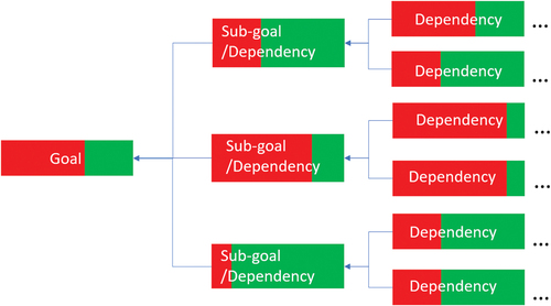
In this model, the graph consists of nodes representing goals, including sub-goals and acyclic edges that signify the probabilistic dependency relationship. Travelling from right to left, where the leftmost node is the ‘goal’ or ‘root’ , the success probability of a root node is determined based on the success probabilities of its ‘parent’ nodes. Within this model, the rightmost nodes, without any parents, are the ‘leaf’ nodes. They are known as ‘uncontrollable’ nodes, meaning that the availability of such nodes is out of the control of the system owners. The colour coding employed in the model illustrates that the red segment represents the probability of not achieving the required state of the goal or sub-goal. In contrast, the green segment represents the probability of attaining the desired state

While DM features robust techniques, its application for risk identification in ICS is currently limited. These limitations hinder the complete adaptation of DM for this of addressing the interactive complexity and tight coupling phenomena:

• Notably, DM falls short in providing a comprehensive analysis of the broader system’s impact and lacks a formalised approach to measure both the direct and indirect consequences of a state change on other parts of the model tree. Additionally, it lacks the formalism required to stochastically test multiple and independent failures in a complex system, a common occurrence in ICS environments.

• DM can only reveal the impact on its branch but cannot understand or accurately assess any direct or indirect impact of a state change on other parts of the model tree.

• DM techniques are limited in their ability to analyse multiple simultaneous or sequential changes in independent nodes within the model. Due to interactive complexity and tight coupling phenomena, this limitation restricts the comprehensive analysis that can be achieved through DM.

• Operationally, the DM technique could be more resource-efficient if it were to perform extended statistical analysis, such as causal inference and predictions in a substantial ICS estate.

BN exhibits some features that give it notable advantages over DM; hence, its adoption by researchers as a robust technique for modelling and managing risk, uncertainty, and decision-making [23]. Similar to DM, BN represents relationships among variables and their dependencies through a DAG. However, BN has the additional capability to allow each variable to take on a finite set of values and conditional dependency between two variables. Furthermore, it allows the learning of the joint probability distribution of all variables of interest, thereby enabling probabilistic modelling, which is perfect for causal reasoning, risk prediction, and decision-making under uncertainty [24]. This is possible using Bayes’ theorem, which states that the probability of an event occurring given some evidence is proportional to the prior probability of the event and the probability of the evidence given the event.

BN, as a member of the family of probabilistic graphical models (PGMs), is a practical choice for risk identification. Its ability to efficiently handle large amounts of uncertain and incomplete data, a common scenario in risk management, is a significant advantage. By leveraging PGM, BN can identify variables that are most likely to contribute to the risk profile and quantify the level of risk associated with each variable reliably. Moreover, BN’s capability to capture the intricate relationships between variables in such systems enhances the accuracy and comprehensiveness of risk identification.

BN often starts with a graph based on an expert understanding of causal relationships among parameters. However, BN has an advantage because it explicitly encodes the independence of distributions from its predecessors. In a BN, each parameter’s probability distribution is determined by a subset of preceding parameters, chosen such that knowing this subset makes the distribution independent of the other predecessors. This subset defines the incoming arcs for each node in the graph. When applied to dependency modelling, BN can use causal inference to identify the most critical and relevant variables, making the relationships clearer and more manageable.

2.1. Related work

In identifying related work, the focus was on research and tools that used probability inference to analyse relationships and dependencies among components in complex systems.

2.1.1. Generic

Both [25] and [26] presented a generic overview of BN. On the one hand [25], provided a framework for developing comprehensive models of CPSs that can be used to discover and analyse interdependencies among different components. On the other hand [26], provided an overview of the literature on the use of BNs for risk assessment and management and discussed the advantages and limitations of BNs for risk analysis. Although these publications offered a generic overview, they did not address DM and the application of BN as a method to enhance its capabilities.

2.1.2. Techniques

Mo et al. [27] proposed a BN-based approach to evaluate cyber risk via the construction of a security risk score model which employs a set of probabilistic values for capturing the inter-dependencies between threats and vulnerabilities in the network. Similarly [28], utilised BN to capture the severity, scope, and potential countermeasures of network intrusion events in real-time. Both approaches explored the dependency relationship between components but did not use causal inference to analyse the relationship or the impact of network intrusion.

2.1.3. Risk

CyberRiskDELPHI was proposed by [29] as a modified version of the Delphi method to address the dynamic threat landscape of mission-critical systems. Subjectivity and variability in cyber risk assessment for mission-critical systems. The authors demonstrated the use of CyberRiskDELPHI for risk identification and prioritisation, but the work did not address the identified phenomena in ICS. Both [30] and [31] focused on the application of BN to risk assessment. While [31] proposed the use of BN in risk assessment for oil and gas processing equipment [30], proposed a BN-based method to validate and improve risk assessment and decision-making process. Neither of these research works provides a focus on risk identification nor addresses the issue of interactive complexity and tight coupling concerning complex systems.

2.1.4. Tools

There exist three commercial tools for building Bayesian network models and performing probability inference: Netica [32], AgenaRisk [33], and Genie [34]. All these software support building Bayesian network models using a graphical interface that specifies variable relationships assigns probability distributions to variables and performs probabilistic inference to calculate outcome probabilities. Sensitivity analysis is also provided in all three tools, enabling the identification of the most significant variables in the model and evaluation of the robustness of the results to altered model parameters. While sharing similar principles with our proposed approach, these three commercial tools differ in their outcomes. They are suited only for less complex models, whereas our proposed tool offers scalability and the ability to handle large and complex models. Moreover, the three tools are incapable of analysing multiple independent nodes.

3. Our approach

To understand the interactive complexity and tight coupling characteristics of a complex system, our research constructs a model capable of sufficiently describing the system’s current state and reflecting the dependency relationships between components and tasks. This is built as a statistical, computational model that relies on the overall function of the system and how the presence (or absence) of each component impacts the overall goal. To achieve this, RiskED was developed as a new approach that integrates four multivariate methods and techniques within a unified model-fitting framework for modelling a DAG causal system by applying BN and causal inference principles to DM to infer connections among unrelated events and reveal concealed insights. In this approach, we leveraged and upheld the underlying assumption of BN that the occurrence of Event B following Event A indicates causal influence from A to B, rather than assuming a specific temporal order between events A and B [35]. By considering both events as distinct and independent occurrences within the BN framework, their relationship can effectively be analysed, and meaningful insights can be uncovered.

To comprehend the interactive complexity and tightly coupled characteristics inherent in a complex system, the research endeavours to construct a model that effectively describes the system’s current state while reflecting the dependency relationships among its components and tasks. This model is developed as a statistical and computational framework that relies on the overall functionality of the system and the impact of each component’s presence or absence on the overarching objective. RiskED is underpinned by a set of proprietary scripts developed in Python and using Python libraries to manipulate data. RiskED accepts variables or nodes to include in a causal model. Attributes of these variables include name, dependency relationship (children and/or parents), and the probability of their state (availability).

The DAG principle was used to transform these variables into a dependency model, revealing the interdependencies among nodes and events. The dependency model is illustrated through an abstract model that captures the relationship between a goal and its dependent components, as well as the dependencies among these components and subsequent dependencies that follow. The process flow of RiskED is illustrated in Figure 2, and the following are the explanations for each step in the process flow:

Figure 2. RiskED process flow.

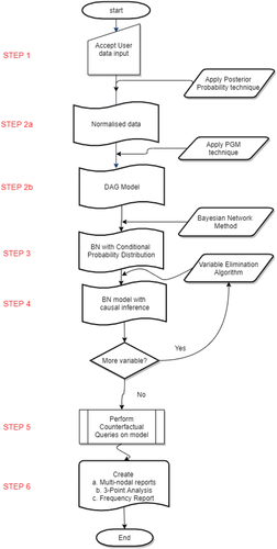
• STEP 2b: BN belongs to the PGM family, which employs edges to represent direct causal relationships between variables [30]. PGMs provide a compact and interpretable representation of dependencies, enabling efficient inference and handling of uncertainty. Leveraging PGM techniques enables the identification of variables that are most likely to contribute to the risk profile and reliably quantifies the associated risks for each variable [24]. The intricate relationships between variables in the model were captured in a DAG model, leading to a more comprehensive and accurate risk identification [36,37]. The result of this Step is the DAG model.

• STEP 3: To investigate the dependencies and the strength of coupling, BN methodology is integrated into RiskED to compute the conditional probability of unknown variables based on observed values of other variables. RiskED assumes that each random variable is independent of its non-descendants when its parents are known. Each node has a set of associated variables known as its parents, which describe cause-and-effect relationships between the parents and the variable (child). Here, each node in the model is treated as conditionally independent of the other. Each node can be in either of two states: $S_0$ and $S_1$, where $S_0$ represents a failed state and $S_1$ represents an optimum functional state. RiskED represents each node as a TabularCPD python class object in a graphical model [36]. The result of this Step is the BN with conditional probabilities.

• STEP 4: To draw probabilistic inferences about the BN model, the result obtained in Step 3 is passed to the Variable Elimination (VE) algorithm. VE provides a systematic inference approach to calculating the marginal probabilities of a target variable by eliminating the other network variables that are irrelevant to the target variable. It is one of the inference algorithms used in BN for probabilistic reasoning. The VE algorithm proceeds by iteratively eliminating variables from the joint distribution, exploiting the conditional independence relationships encoded in the graphical model.

• STEP 5: This is a pivotal step in the process. It involves building hypothetical ‘what-if’ scenarios based on the causal relationships within the Bayesian network result of Step 4. The aim is to understand the potential consequences of different interventions. This is achieved by determining how the values of certain variables would change if other variables were set to different values. The step requires identifying the variables to intervene on and setting them to the desired values. These are the variables used to estimate the resulting changes.

• This process flow is further explained with Algorithm 1, which describes Steps 2, 3, and 4 and how Variable Elimination (VE) was adapted to compute inference in RiskED.

Algorithm 1. RiskED Process Flow

1: procedure transform

2:      global root infer, labellist, t0

3:      f ← open(”posterior.csv”, ”rt”, encoding = ”utf − 8”)

4:      for x in range(len(valuea)) do

5:            valueb.append(round(float(1 − valuea[x]), 4))

6:      end for

7:      values ← [valueb, valuea]

8:      if len(evidence) == 0 then

9:            model.add node(labellist[num])

10:          cpd[num] ← TabularCPD(variable = labellist[num], variable card = 2, values = values)

11:         model.add cpds(cpd[num])

12:    else

13:        model.add node(labellist[num])

14:       for x in range(len(evidence)) do

15:           model.add edge(evidence[x], labellist[num])

16:       end for

17:      cpd[num] ← TabularCPD(variable = labellist[num], variable card = 2, values = values, evidence = evidence, evidence card = evidence card)

18:      model.add cpds(cpd[num])

19:    end if

20:    root infer ← VariableElimination(model)

21:    rootvariable ← root infer.query(variables = [labellist[0]])

22:    t0 ← rootvariable.get value(labellist[0], 1)

23: end procedure

24: return

As an illustration, Figure 3 presents a high-level depiction of the dependency model utilised in this research study. In this model, the variable Secured system serves as the primary goal (root node), while its dependencies (parents) include variables such as SPE1, SPE2, SPE3, SPE4, SPE5, SPE6, SPE7, and SPE8. Similarly, the node labelled SPE2 relies on both the Inventory management and Change control nodes.

Figure 3. High-level depiction of the dependency model.

Due to the complexity and size of the complete dependency model, it is impractical to display it in its entirety within this paper; instead, the model is available in PNG format at this https://git.cardiff.ac.uk./c1001323/RiskED/-/blob/main/eDependency.pnglink

To investigate these dependencies and the level of coupling, BN methodology is integrated to compute the conditional probability of unknown variables based on observed values of other variables. RiskED assumes that each random variable is independent of its non-descendants when its parents are known. Each variable has a set of associated variables known as its parents, which describe cause-and-effect relationships between the parents and the variable (child). Here, each variable in the model is treated as conditionally independent of the other, and each variable can be in either of two states: $S_0$ and $S_1$, where $S_0$ represents a failed state and $S_1$ represents a functional state. RiskED represents each variable as a TabularCPD python class object in a graphical model [36]. For instance, the TabularCPD for the Secured System variable is defined as a variable with two states. It has eight parents, each of which can be in two states. Consequently, the probability value associated with the Secured System variable combines 32 ($8\times 2\times 2$) arguments or possible outcomes. This probability value reveals additional information not available to decision makers [36].

Causal inference provides system owners with the knowledge of which uncontrollable factor holds the greatest positive or negative impact on the overall goal’s state. It serves as a crucial element in comprehending the most significant risk location in the model. Based on the VE algorithm, the inference query to obtain the hidden data from the model is in the form of $\mathit{P}(\mathit{Y}|\mathit{E}=\mathit{e})$ where Y and E are disjoint variables in the model, and E is observed taking value e [36,38]. As an example in the data used in this research, $\mathit{P}(\mathit{SecuredSystem}|\mathit{SPE}1=0)$ is interpreted as: ‘What is the probability of the Secured System given that SPE1 fails or is not available?’  With causal inference, the current state of the system is already known. We, therefore, choose counterfactual scenarios to perform a ‘what-if’ analysis.

4. Case study and analysis

The subject of this case study is a process-driven manufacturing enterprise operating on the IEC 62,443 framework for industrial automation and control systems security [39]. Within this framework, roles and processes are well-defined, and the responsibility for the overall cyber security program lies with the Board. Additionally, business and process owners are accountable for the security of their respective segments.

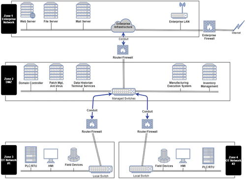
The network segmentation and control follows the ‘zones’ and ‘conduits’ concepts to isolate critical systems and control the flow of information, enhancing security and reducing the potential impact of cyber threats. ‘zones’ represent logical or physical divisions within an ICS network that group together devices and systems with similar security requirements for the purpose of providing separation and control between different areas of the network to limit the impact of potential cyber threats.

The case study comprises three zones, namely: Enterprise Network Zone, Demilitarise Zone (DMZ) and OT Network zone, as shown in Figure 4. ‘Conduits’ serve as controlled entry and exit points for data flow between zones while enforcing security policies and preventing unauthorised access. ‘Conduit’ ensure that only authorised communication is permitted and that traffic is inspected and filtered according to predetermined rules and policies [39,40]. The operational activities of the case study are segmented into independent zones and connected using conduits.

Figure 4. Communication network segmentation showing zones and conduits.

4.1. Data

The data utilised in this study was acquired from a risk assessment conducted on the operational technology (OT) security practices within the ICS enterprise. In accordance with the IEC 62,443 standard’s functional requirements (FR), there are eight secure, productive environments (SPE) criteria that offer guidance for achieving and maintaining a secure and productive environment. The risk assessment measures maturity against the FR capabilities within the SPE, evaluating the cyber security profile of the environment and assigning scores based on a four-scale maturity level: 1 - Initial, 2 - Managed, 3 - Defined, and 4 - Improving. As shown in Table 2, the goal of the assessment is to measure the system’s overall security.

Table 2. Risk assessment data based on IEC 62,443 method.

SPE 1			SPE 2
	Maturity			Maturity
Control	Desired	Actual	Control	Desired	Actual
ORG 1 – Security related organisation and policies			CM 1 – Inventory management of IACS hardware/software components and network communications
ORG 1.1: Information security management system (ISMS)	3	2	CM 1.1: Asset inventory baseline	3	3
ORG 1.2: Background checks	3	2	CM 1.2: Infrastructure drawings/documentation	3	3
ORG 1.3: Security roles and responsibilities	3	2	CM 1.3: Configuration settings	3	3
ORG 1.4: Security awareness training	3	2	CM 1.4: Change control	3	3
ORG 1.5: Security responsibilities training	3	2
ORG 1.6: Supply chain security	3	2
ORG 2 – Security assessments and reviews
ORG 2.1: Security risk mitigation	3	2
ORG 2.2: Processes for discovery of security anomalies	3	2
ORG 2.3: Secure development and support	3	2
ORG 2.4: SP reviews	3	2
ORG 3 – Security of physical access
ORG 3.1: Physical access control	4	4
SPE 3			SPE 4
NET 1 – System segmentation			COMP 1 – Devices and media
NET 1.1: Segmentation from non-IACS networks	3	2	COMP 1.1: Device hardening	2	0
NET 1.2: Documentation of network segment interconnections	3	2	COMP 1.2: Dedicated portable media	2	1
NET 1.3: Network segmentation from safety systems	3	2	COMP 2 – Malware protection
NET 1.4: Network autonomy	3	2	COMP 2.1: Malware free	2	0
NET 1.5: Network disconnection from external networks	3	2	COMP 2.2: Malware protection	2	0
NET 1.6: Internal network access control	3	2	COMP 2.3: Malware protection software validation and installation	2	0
NET 1.7: Device connections	3	2	COMP 3 – Patch management
NET 1.8: Network accessible services	3	2	COMP 3.1: Security patch authenticity/integrity	2	0
NET 1.9: User messaging	3	2	COMP 3.2: Security patch validation and installation	2	0
NET 1.10: Network time distribution	3	2	COMP 3.3: Security patch status	2	0
NET 2 – Secure wireless access			COMP 3.4: Security patching retention of security	2	0
NET 2.1: Wireless protocols	2	0	COMP 3.5: Security patch mitigation	2	0
NET 2.2: Wireless network segmentation	2	0
NET 2.3: Wireless properties and addresses	2	0
NET 3 – Secure remote access
NET 3.1: Remote access applications	3	2
NET 3.2: Remote access connections	3	2
NET 3.3: Remote access termination	3	2
SPE 5			SPE 6
DATA 1 – Protection of data			USER 1 – Identification and authentication
DATA 1.1: Data classification	2	2	USER 1.1: User identity assignment	2	2
DATA 1.2: Protection of data	2	2	USER 1.2: User identity removal	2	2
DATA 1.3: Safety system configuration mode	2	2	USER 1.3: User identity persistence	2	2
DATA 1.4: Failure-state	2	2	USER 1.4: Access rights assignment	2	2
DATA 1.5: Data retention	2	2	USER 1.5: Least privilege	2	1
DATA 1.6: Data purging	2	2	USER 1.6: Software service authentication	2	2
DATA 1.7: Cryptographic mechanisms	2	2	USER 1.7: Software services interactive login rights	2	2
DATA 1.8: Key management	2	2	USER 1.8: User authentication	2	2
DATA 1.9: Public key infrastructure (PKI)	2	2	USER 1.9: Multifactor authentication	2	1
			USER 1.10: Mutual authentication	2	2
			USER 1.11: Password protection	2	1
			USER 1.12: Shared and disclosed/compromised passwords	2	1
			USER 1.13: User login display information	2	1
			USER 1.14: User login failure displays	2	1
			USER 1.15: Consecutive login failures	2	2
			USER 1.16: Session integrity	2	1
			USER 1.17: Concurrent sessions	2	2
			USER 1.18: Screen lock	2	2
			USER 2 – Authorisation and access control
			USER 2.1: Authorisation	2	1
			USER 2.2: Administrative rights authorization	2	1
			USER 2.3: Multiple approvals	2	1
			USER 2.4: Manual elevation of privileges	2	1
SPE 7			SPE 8
EVENT 1 – Event and incident management			AVAIL 1 – System availability and intended functionality
EVENT 1.1: Event detection	2	1	AVAIL 1.1: Continuity management	2	1
EVENT 1.2: Event reporting	2	1	AVAIL 1.2: Resource management	2	1
EVENT 1.3: Event reporting interfaces	2	1	AVAIL 1.3: DoS attacks	2	1
EVENT 1.4: Logging	2	1	AVAIL 2 – Backup/restore/archive
EVENT 1.5: Log entries	2	1	AVAIL 2.1: Backup	2	1
EVENT 1.6: Log access	2	1	AVAIL 2.2: Backup non-interference	2	1
EVENT 1.7: Event analysis	2	1	AVAIL 2.3: Backup verification	2	1
EVENT 1.8: Incident handling and response	2	1	AVAIL 2.4: Backup media	2	1
EVENT 1.9: Vulnerability handling	2	1	AVAIL 2.5: Backup restoration	2	1

The goal was labelled Secured System (not shown in the table), whose dependencies are the eight SPEs. The Control column is the name of each FR. For example, there are three groups of FRs in SPE1 (in bold letters), each with dependent FRs. For each FR, there are two maturity values; ‘Desired’ and ‘Actual’. The process or business owners have previously determined the ‘Desired’ maturity state based on the overall goal of the enterprise. The desired maturity is the target they want to attain. The ‘Actual’ maturity value is assessed based on penetration testing, system logs, cyber security policies, vulnerability and threat analysis, observations, operator experience, and interviews. So the Background checks FR has a desired maturity of 3 and actual maturity of 2, while Physical access control has a value of 4 for both maturities. There are a total of 114 components (variables) in the data.

To convert the risk assessment values to probability values, the ‘Actual’ Maturity value is normalised against the ‘Desired’ Maturity values, translating the scores into corresponding probability values between zero and one (0–1). For example, the actual value of Background checks translates to 67% ($2/3=0.67$) and Physical access control to 100% ($4/4=1$).

A dependency model that shows the interdependencies among the various components of the SPE criteria was built using a structured table format with the following attributes:

• Label: A numeric value used as an identifier to represent the node name. The full list of labels and corresponding node names is available in a CSV format at this https://git.cardiff.ac.uk./c1001323/RiskED/-/blob/main/modellist.csvlink

• Node: The components comprising the model.

• Child Node: Child Nodes depend on other nodes.

• Dependants: The number of child nodes that depend on this node.

• Probability: The maturity values converted to probability values.

The full data is available in a CSV format at this https://git.cardiff.ac.uk./c1001323/RiskED/-/blob/main/Converted_data.csvlink

Table 3 shows the analysed model. There are three types of nodes in this table, namely, the root node, leaf nodes, and child nodes. The root node is the goal of the model, Child nodes rely on other nodes, while leaf nodes are the nodes without dependants (zero values in the Dependants column). In addition, child nodes have values greater than zero in the Dependants column. It is worth noting that, given the hierarchical nature of the dependency model, a child node may also act as a parent to other nodes.

Table 3. Case study: dependency model.

Label	Node	Child Node	Dependants	Probability
0	Secured System		8	0.011
1	SPE1	Secured System	3	0.5366668
2	SPE2	Secured System	1	0.9942488
3	SPE3	Secured System	3	0.01
4	SPE4	Secured System	3	0.01
11	Security of Physical Access	SPE1	1	0.9985591
12	Information Security Management System (ISMS)	Security Related Organisation and Policies	0	0.9333333
13	Background Checks	Security Related Organisation and Policies	0	0.9333333
14	Security Roles and Responsibilities	Security Related Organisation and Policies	0	0.9333333
28	System Segmentation	SPE3	10	0.2426199
48	Malware Protection	SPE4	3	0.0010323
103	Vulnerability handling	Event and incident management	0	0.7667
104	System availability and intended functionality	SPE8	3	0.4506884
105	Backup/restore/archive	SPE8	5	0.2649277
109	Backup	Backup/restore/archive	0	0.7667
110	Backup non-interference	Backup/restore/archive	0	0.7667
111	Backup verification	Backup/restore/archive	0	0.7667
112	Backup media	Backup/restore/archive	0	0.7667
113	Backup restoration	Backup/restore/archive	0	0.7667

To normalise the values associated with leaf nodes, the posterior probability technique proposed by [41] was utilised, resulting in the Probability column within Table 3. The probability values in black letters are normalised values, and those in red letters are computed values using PGM techniques.

To interpret the entry for each node, it can be read as follows:

• The probability of Backup restoration (label 113) being in the desired state is 76.7%, or

• The probability of SPE1 (Label 1) achieving the desired state is 53.6%.

4.2. Analysis

RiskED was used to apply the axioms of Bayesian networks to the data presented in Table 3. By employing this approach, we computed both conditional probability and joint probability values for each node within the model. Our primary focus was on the marginal probability, which represents the present state of the overall model. Specifically, the probability of the Secured System attaining the desired state is 0.32956%. This value signifies the current condition of the system and serves as a crucial factor for all subsequent analyses conducted on the model. We subsequently performed causal inference counterfactual queries on the model to know how the overall goal (Secured System) is affected in different scenarios. Specifically, we want to understand the following:

• What is the impact on the model’s state if a single component fails or becomes unavailable versus when the same component is fully functional? In other words, what happens to the model if the actual maturity of a specific node is 0% or if the actual maturity equals the desired maturity (i.e. 100%)?

• What is the impact on the model’s state if multiple stochastic components fail or become unavailable versus when the same components are fully functional? This query addresses the interactive complexity and tight coupling phenomena.

Using VE to obtain causal inferences and counterfactuals for single and multi nodes combinations analysis, we present the results obtained for single-node analysis, as well as two- and three-nodal combinations, in the Tables 4, 5, and 6. Here, the top 10 most sensitive (negative) nodes are included. An explanation of each column in the tables is as follows:

• Node label: This label corresponds to each node name in the model.

• Marginal Probability: This represents the probability of the model as mentioned previously. It reflects the current true state of the system in the present time.

• P(G|E1 = 0) This denotes the causal inference of a new probability for the Secured System, given that the state or event (E) of a specific node is 0 (unavailable). Here, we determine the probability of achieving the goal when a single node or a combination of nodes is turned off or failed. This value represents a probability.

• P(G|E1 = 1) This refers to the causal inference of a new probability for the Secured System, given that the state of a specific node is 1 (100% present). In this case, we compute the probability of achieving the goal when a single node or a combination of nodes is set to 100% availability. This value represents a probability.

• P1 This indicates the normalised difference between the marginal probability and the computed causal inference when the node is absent. It is computed as the marginal probability minus the value of P(G|E1 = 0).

• P2 This represents the normalised difference between the computed causal inference when the node is fully present and the marginal probability. It is computed as the value of P(G|E1 = 0) minus the marginal probability.

Table 4. Causal inference with single node.

Node Label	Marginal Probability	$\mathit{P}(\mathit{G}|$ E1=0)	$\mathit{P}(\mathit{G}|$ E1=1)	P1	P2
[24]	0.32957	0.00420	0.32989	0.98742	0.01258
[25]	0.32957	0.00420	0.32989	0.98742	0.01258
[26]	0.32957	0.00420	0.32989	0.98742	0.01258
[27]	0.32957	0.00420	0.32989	0.98742	0.01258
[66]	0.32957	0.02002	0.33050	0.94289	0.05711
[65]	0.32957	0.02002	0.33050	0.94289	0.05711
[63]	0.32957	0.02002	0.33050	0.94289	0.05711
[62]	0.32957	0.02002	0.33050	0.94289	0.05711
[61]	0.32957	0.02002	0.33050	0.94289	0.05711
[64]	0.32957	0.02002	0.33050	0.94289	0.05711

Table 5. Causal inference with two nodes.

Node Label	Marginal Probability	$\mathit{P}(\mathit{G}|$ E1&E2=0)	$\mathit{P}(\mathit{G}|$ E1&E2=1)	P1	P2
[26+66]	0.32957	0.00003	0.33082	0.99992	0.00008
[26+67]	0.32957	0.00003	0.33082	0.99992	0.00008
[24+60]	0.32957	0.00003	0.33082	0.99992	0.00008
[24+61]	0.32957	0.00003	0.33082	0.99992	0.00008
[24+62]	0.32957	0.00003	0.33082	0.99992	0.00008
[24+63]	0.32957	0.00003	0.33082	0.99992	0.00008
[24+64]	0.32957	0.00003	0.33082	0.99992	0.00008
[24+65]	0.32957	0.00003	0.33082	0.99992	0.00008
[24+67]	0.32957	0.00003	0.33082	0.99992	0.00008
[27+66]	0.32957	0.00003	0.33082	0.99992	0.00008

Table 6. Causal inference with three nodes.

Node Label	Marginal Probability	$\mathit{P}(\mathit{G}|$ E1,E2,E3=0)	$\mathit{P}(\mathit{G}|$ E1,E2,E3=1)	P1	P2
[24+25+65]	0.32957	0.00023	0.33115	0.99930	0.00070
[25+26+68]	0.32957	0.00023	0.33115	0.99930	0.00070
[24+25+64]	0.32957	0.00023	0.33115	0.99930	0.00070
[25+26+67]	0.32957	0.00023	0.33115	0.99930	0.00070
[25+26+66]	0.32957	0.00023	0.33115	0.99930	0.00070
[25+26+65]	0.32957	0.00023	0.33115	0.99930	0.00070
[25+26+64]	0.32957	0.00023	0.33115	0.99930	0.00070
[25+26+63]	0.32957	0.00023	0.33115	0.99930	0.00070
[25+26+62]	0.32957	0.00023	0.33115	0.99930	0.00070
[25+27+61]	0.32957	0.00023	0.33115	0.99930	0.00070

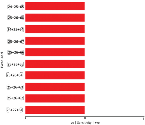
We conducted computations for two-nodal combinations, P(G|E1,E2 = 0) and P(G|E1,E2 = 1), by assigning probabilities of zero and one to nodes E1 and E2. Similarly, we also computed three-nodal combinations, P(G|E1,E2,E3 = 0) and P(G|E1,E2,E3 = 1), by assigning probabilities of zero and one to nodes E1, E2, and E3. The rationale behind these two-nodal and three-nodal analyses is to address the complexity of interactions and the phenomenon of tight coupling. These analyses provide insights into the outcomes when two or three components fail simultaneously or synchronously, even if they are not directly connected.

The columns P1 and P2 in our model represent sensitivity values that have been derived as normalised values to ensure their sum equals 1. These values were used to construct the three-point sensitivity analysis (3PS) for the model as shown in the tornado charts in Figures 5–7. The tornado chart enables the identification of events or variables that have the most influence on the overall outcome. The vertical axis of the tornado chart represents the different events being analysed. Each variable is listed on the axis in descending order of importance. The horizontal axis represents the impact of the events on the outcome. The axis is divided into positive and negative sections, with the zero point in the middle. The length of the bars represents the magnitude of the impact. Each event is represented by a bar in the chart. The length of the bar indicates the impact on the outcome. Longer bars indicate a higher impact, while shorter bars represent a lower impact. The colour of the bars, either red or green, indicates the direction of influence (negative or positive, respectively). The junction between the colour bars reveals the level of sensitivity in relation to the marginal probability (the goal). Furthermore, the sensitivity values offer valuable insights into the potential magnitude of the negative impact that a node can have on the model.

Figure 5. Single node 3-point sensitivity using causal inference.

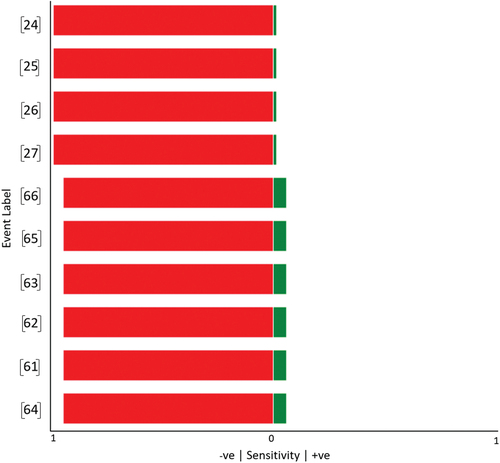
Figure 6. Two-nodal 3-point sensitivity analysis using causal inference.

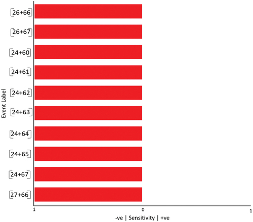
Figure 7. Three-nodal 3-point sensitivity analysis using causal inference.

Analysing Figure 5, we observe that nodes 24, 25, 26, and 27 (Asset Inventory Baseline, Infrastructure Drawings/Documentation, Configuration Settings, and Change Control, respectively) are the most sensitive nodes within the model. Failure of any of these nodes would lead to a significant decrease in the probability of success, dropping from 0.32957% to 0.00420%. Conversely, investing in these nodes would slightly enhance the overall success rate to 0.329895%, as demonstrated in Table 4.

Figure 6 illustrates the outcomes of the top 10 combinations of two nodes that have the greatest negative impact on the probability of achieving the goal. Interestingly, regardless of the specific combination chosen, the top 10 combinations exhibit the same level of impact. For instance, the combination of nodes 26 and 66 (Configuration Settings and Cryptographic Mechanisms) or nodes 24 and 60 (Asset Inventory Baseline and Data Classification) both lead to a significant decrease in the probability of the goal, ‘Secured system’, from 0.32957% to 0.00003%.

These results suggest that there is no tight coupling or direct connection between the chosen combinations of nodes. In other words, the probability of achieving the root node, ‘Secured system’, based on a particular combination of two nodes (e.g. nodes 24 and 60) is independent of the values of other combinations (e.g. nodes 24 and 63). This outcome was expected since the nodes being analysed are leaf nodes. In addition, a 100% improvement in these nodes increased the success rate to 0.33082%

Furthermore, it is worth noting that the sensitivity is higher (in a negative sense) in the two-nodal combinations (0.00003%) compared to the individual node scenario (0.00420%). This indicates that if cyber incidents were to target two nodes simultaneously or sequentially, the risk to the system would be greater.

Among the top 10 in a three-nodal combination, the combinational failure of nodes 24, 25, and 65 (Asset Inventory Baseline, Infrastructure Drawings/Documentation, and Data Purging) or nodes 25, 27, and 61 (Infrastructure Drawings/Documentation, Change Control, and Data Protection) leads to a significant reduction in the probability of achieving the goal, dropping from 0.32957% to 0.00023%. On the other hand, a 100% improvement in these nodes can have a positive impact on the goal, increasing the success rate to 0.33115%, regardless of the specific combination of nodes.

In both Figures 6 and 7, the visibility of the green bars is limited due to the significant difference in the ratio between P1 and P2, as well as the scale of the graphs. Although there is an increase in the probability when the nodes are fully available (100%), the negative impact is substantially higher in comparison.

Following the multi-nodal causal inference analysis, we conducted a frequency analysis to identify the most influential nodes based on their frequency of occurrence in multi-nodal combinations. As presented in Figure 8, node 24 (Asset Inventory Baseline) emerged as the most influential in a 2-nodal combination, occurring seven times, twice as frequently as the next most frequent (node 66), which occurs three times. The frequency results suggest that node 24 possesses higher interactive complexity in comparison to the other nodes.

Figure 8. Two-nodal frequency analysis - negative impact.

In contrast, nodes 25 and 26 are the most influential nodes in a 3-nodal causal inference combination, occurring ten and seven times, respectively, as demonstrated in Figure 9.

Figure 9. Three-nodal frequency analysis - negative impact.

The results of the frequency analysis, depicted in Figures 8 and 9 align with the findings of the single-nodal causal inference analysis presented in Figure 5, with nodes 24 and 25 being identified as highly important in both analyses. This emphasised their significance in contributing to the overall outcome of the goal and underscored the notion that the inclusion or exclusion of any of these nodes can notably impact the model’s performance. Remarkably, the persistent occurrences of these critical nodes across the three graphs within Figures 5–7 suggest the potential confounding variables that may affect the model’s predictability in the absence or alteration of these nodes.

In relation to our scenario, a detailed asset inventory (node 24) and infrastructure documentation (node 25) provide a foundation upon which all other cyber security activities are built. Along with node 26 (Configuration settings), these three nodes form the basis for the second requirement of a secure, productive environment (SPE) under the IEC 62,443 standard, which conveys the idea that it is difficult to safeguard or defend something if you are unaware of its existence or its value. Organisations must be aware of the components, data, and information they possess in order to protect them from unauthorised access or breaches, particularly in complex systems such as ICS, where there are numerous components, including remote locations.

5. Discussions and limitations

System owners gain direct insight into the underlying mechanisms driving a system by examining the relationships between different factors and identifying those directly impacting others. This knowledge can aid in informed decision-making and interventions. One key benefit of our proposed technique is its ability to identify causal relationships between variables. In our study, we utilised this technique to identify crucial factors contributing to a specific outcome and to reveal hidden inferences not directly observable with traditional dependency modelling. Within our scenario, our technique exposed the two characteristics of complex systems discussed in Section 1.

This paper focused on conducting causal inference queries and analysis exclusively on leaf nodes. However, the model structure, as described in Section 4.2, offers the flexibility to expand the scope of queries by incorporating other nodes. This is possible because each node in the Bayesian network is represented as a conditionally independent node, allowing for the inclusion of additional nodes in the analysis.

There are several noteworthy observations from this research that project limitations. One key issue is that BNs do not inherently provide a mechanism to select a prior. To address this, we employed a novel technique that allowed us to calculate the posterior probability for the nodes. Another issue is that causal inference with DM is based on the assumption that relationships between variables remain stable over time. However, as can occur in complex systems, the relationships between variables may change over time, resulting in inaccurate predictive models. To address this, we propose a risk identification process that can be triggered automatically in the event of changes to the component of the model. Furthermore, two- and three-combination queries were used as a proof of concept, and while effective in identifying significant factors, the computational complexity increased significantly. With a dataset of 114 nodes, including 89 leaf nodes, a two-combinational query produced over 3000 combination results, while a three-combinational query resulted in over 100,000 combinations. Clearly, extending this technique to more complex, larger models presents significant computational challenges.

This limitation became apparent in RiskED because automated causal inference requires a repeated operation that’s carried out on the full collection of leaf nodes in the model. The computational complexity of the RiskED’s algorithm involves iterations roughly proportional to the factorial of the number of leaf nodes, represented as O(X!). In this context, the Big O symbolises the maximum growth rate of the algorithm function. The computational challenge of O(X!), where X! represents the factorial of X, is that the factorial function grows extremely rapidly as X increases, making algorithms with a time complexity of O(X!) highly computationally intensive.

The factorial of a number X is the product of all the positive integers less than or equal to X. Mathematically, it is represented as:

$\mathit{O}(\mathit{X}!)=\mathit{x}\times [\mathit{x}-1]\times [\mathit{x}-2]\times \dots \times 3\times 2\times 1$

Where:

• x is the total number of leave nodes

• O(X!) is the factorial time complexity, which is incredibly inefficient

6. Conclusion and future work

Our research is aimed at improving the capacity of DM to effectively assess the impact of system risks and detect unpredictable phenomena. While DM is an established technique in the field of cyber risk assessment, it has limitations when dealing with complex systems due to the difficulty of establishing explicit probability distributions across all branches of the model. To address this issue, we proposed RiskED as an approach that leverages the capabilities of Bayesian networks to enhance the capability of DM by incorporating inferences. The application of RiskED was tested and evaluated using a small sample of data from an ICS manufacturing environment. The results of this proof-of-concept demonstration highlighted the potential of the RiskED approach to scale up to more comprehensive models, providing interpretable and repeatable results for cyber risk identification. This indicates RiskED’s capacity to significantly improve upon existing risk identification techniques used in ICS contexts.

Specifically, the approach enabled the successful identification and analysis of previously unknown risks associated with the interactive complexity and tight coupling phenomena prevalent in ICS environments. These types of risks can potentially lead to unpredictable system behaviours and out-of-control events. By incorporating a suite of enhanced techniques, RiskED was able to adapt and improve the capability of DM to address these complex cyber risk identification challenges.

Further research and development are needed to fully explore and optimise the capabilities of RiskED and to broaden its applications in the field of cyber risk identification. In future research, we intend to explore innovative computational approaches that can efficiently manage the resources in analysing large datasets. One such approach is the System-thinking approach that identifies negligible nodes and empowers asset owners to select a combination of nodes from the model’s complete list of nodes to minimise computation time spent in identifying all possible combinations within the model, albeit at the cost of performing single sets of combinations at a time. While a promising step forward, further work is needed to determine its efficacy. In addition to further exploring efficient computational approaches, we seek to leverage RiskED to make predictions about future outcomes based on past data and develop predictive models to forecast future cyber risk trends. Doing so would enable organisations to better plan for potential threats and vulnerabilities and make more informed decisions.

Overall, we believe that the application of this approach can contribute meaningfully to the enhancement of cyber risk management in complex system environments.

Acknowledgments

This work has been supported by the Knowledge Economy Skills Scholarships (KESS2) - a major pan-Wales operation supported by European Social Funds (ESF) through the Welsh Government and Thales UK.

Disclosure statement

No potential conflict of interest was reported by the author(s).

Data availability statement

All data is provided in full in the results section of this paper. No new data was created during this study.

Additional information

Funding

The work was supported by the EPSRC [EP/W003325/1].

Notes on contributors

Ayodeji O. Rotibi

Ayodeji O. Rotibi received the B.SC. degree in computer science from the University of Benin, Nigeria, in 1990 and the M.Sc. degree in computer system security from the University of Glamorgan, Pontypridd, United Kingdom, in 2006. He also received an M.Sc. degree in information security and privacy from Cardiff University, Cardiff, United Kingdom, in 2018. He has recently completed a PhD degree in cyber security at Cardiff University, Cardiff, UK. His research interests include cyber risk assessment and analysis in complex environments and the development of tools to simplify cyber risk identification.

Neetesh Saxena

Neetesh Saxena is currently an Associate Professor in Cyber Security with the School of Computer Science and Informatics at Cardiff University, United Kingdom, with 17-plus years of teaching/research experience. Before joining Cardiff University, he was an Assistant Professor at Bournemouth University, United Kingdom. Prior to this, he was a post-doctoral researcher at the School of Electrical and Computer Engineering at the Georgia Institute of Technology, USA, and with the Department of Computer Science at Stony Brook University, USA, and SUNY Korea. He was a DAAD Scholar at Bonn-Aachen International Center for Information Technology (B-IT), Rheinische-Friedrich-Wilhelms Universität, Bonn, Germany and a TCS Research Scholar. His current research interests include cyber security and critical infrastructure security, including cyber-physical system security: smart grid, V2G and cellular communication networks

Pete Burnap

Pete Burnap is a professor of data science and cyber security at Cardiff University, United Kingdom. He is the Director of Cardiff’s NCSC/EPSRC Academic Centre of Excellence in Cyber Security Research. He also leads artificial intelligence for cyber security research at Airbus DTO. His research interests include socio-technical security and the understanding of risks to society from cyber-enabled systems.

Craig Read

Craig Read is the Head of Engineering and Research and is part of the Thales SIX Technical Directorate. In his role as Head of Engineering and Research, Craig is responsible for the definition of engineering and research strategy as well as setting up the engineering process, controls and governance needed to deliver projects. Craig also works alongside clients, delivering presentations and developing proposals to help them achieve their goals. Craig is a respected technical architect and consultant with a wealth of experience and a proven track record within network solutions, PKI, key management, tactical data links, data management/control/protection, service provision and general cyber security with over 15 years” extensive experience in both military and government systems and communications.

References

- NCSC. Risk management guidance. 2017 [cited 2022 May 30]. Available from: https://tinyurl.com/47mym4nz
- Hagerott M. Stuxnet and the vital role of critical infrastructure operators and engineers. Int J Crit Infrastruct Prot. 2014;7(4):244–246. doi: 10.1016/j.ijcip.2014.09.001
- Lee R. The sliding scale of cybersecurity. Rockville, USA: SANS Institute; January 2015; 24:2018.
- Parsons D. Five startling findings in 2023’s ics cybersecurity data. 2023 [cited 2024 Feb 27]. Available from: https://tinyurl.com/czwbbk9v
- Wolf FG. Operationalizing and testing normal accident theory in petrochemical plants and refineries. Prod Ops Manag. 2001;10(3):292–305. doi: 10.1111/j.1937-5956.2001.tb00376.x
- Perrow C. Normal accidents: living with high risk technologies - updated edition. Revised ed. New Jersey, USA: Princeton University Press; 1999.
- Ten C, Manimaran G, Liu C. Cybersecurity for critical infrastructures: attack and defense modeling. IEEE Trans Syst Man Cybern A. 2010;40(4):853–865. doi: 10.1109/TSMCA.2010.2048028
- Duggan D, Berg M, Dillinger J, et al. Penetration testing of industrial control system. 2005 [cited 2022 Mar 20]. Available from: https://tinyurl.com/3t9tvrre
- Hirsch GB, Levine R, Miller RL. Using system dynamics modeling to understand the impact of social change initiatives. Am J Community Psychol. 2007;39(3–4):239–253. doi: 10.1007/s10464-007-9114-3
- Ahmed D, Diaz E, Domínguez J. Novel multi-imu tight coupling pedestrian localization exploiting biomechanical motion constraints. Sensors. 2020;20(18):53–64. doi: 10.3390/s20185364
- Sullivan JE, Kamensky D. How cyber-attacks in Ukraine show the vulnerability of the us power grid. The Electricity J. 2017;30(3):30–35. doi: 10.1016/j.tej.2017.02.006
- Tvedt IM. A conceptual exploration of a collaborative environment in the construction industry when working with temporary socio-technical processes. In: Pasquire C, and Hamzeh F, editors. Proc. 27th Annual Conference of the International Group for Lean Construction (IGLC). Dublin, Ireland. 2019. p. 785–796.
- Ding D, Han Q, Wang Z, et al. A survey on model-based distributed control and filtering for industrial cyber-physical systems. IEEE Trans Ind Inf. 2019;15(5):2483–2499. doi: 10.1109/TII.2019.2905295
- Hubbard DW, Seiersen R. How to measure anything in cybersecurity risk. New Jersey, USA: John Wiley & Sons; 2016.
- Cox AL Jr. What’s wrong with risk matrices? Risk analysis. An Int J. 2008;28(2):497–512. doi: 10.1111/j.1539-6924.2008.01030.x
- Ball DW, Watt J. Further thoughts on the utility of risk matrices. Risk Anal. 2013;33(11):2068–2078. doi: 10.1111/risa.12057
- Elhady AM, El-Bakry HM, Abou Elfetouh A. Comprehensive risk identification model for scada systems. Secur Commun Network. 2019;2019:1–24. doi: 10.1155/2019/3914283
- Kordy B, Kordy P, Mauw S, et al. Adtool: security analysis with attack–defense trees. In: International Conference on Quantitative Evaluation of Systems. Buenos Aires, Argentina: Springer; 2013. p. 173–176.
- Young W, Leveson N. Systems thinking for safety and security. In: Proceedings of the 29th Annual Computer Security Applications Conference; (NY), NY (USA). Association for Computing Machinery; 2013. p. 1–8; ACSAC ‘13. doi: 10.1145/2523649.2530277
- Slater D. Open group standard dependency modelling. 2016 [cited 2022 Mar 20]. Available from: https://tinyurl.com/4ck8ns45
- Burnap P, Baker C, Gordon J, et al. Dependency modeling. 2012 [cited 2022 Jan 15]. Available from: https://publications.opengroup.org/c133
- Slater D. A dependency modelling manual - working paper. 2016 [cited 2022 Mar 20]. Available from: https://tinyurl.com/2p9jp2b4
- Gupta A, Slater JJ, Boyne D, et al. Probabilistic graphical modelling for estimating risk of coronary artery disease: applications of a flexible machine-learning method. Med Decis Making. 2019;39(8):1032–1044. doi: 10.1177/0272989X19879095
- Koller D, Friedman N. Probabilistic graphical models: principles and techniques. Cambridge, MA, USA: MIT press; 2009.
- Akbarzadeh A, Katsikas S. Towards comprehensive modeling of cpss to discover and study interdependencies. In: Computer Security. ESORICS 2022 International Workshops: CyberICPS 2022, SECPRE 2022, SPOSE 2022, CPS4CIP 2022, CDT&SECOMANE 2022, EIS 2022, and SecAssure 2022; Copenhagen, Denmark. Springer; 2023. p. 5–25. [2022 Sep 26–30], Revised Selected Papers.
- Kaikkonen L, Parviainen T, Rahikainen M, et al. Bayesian networks in environmental risk assessment: a review. Integr Environ Assess Manag. 2021;17(1):62–78. doi: 10.1002/ieam.4332
- Mo SYK, Beling PA, Crowther KG. Quantitative assessment of cyber security risk using bayesian network-based model. In: 2009 Systems and Information Engineering Design Symposium. Charlottesville, VA, USA: IEEE; 2009. p. 183–187.
- Xie P, Li JH, Ou X, et al. Using bayesian networks for cyber security analysis. In: 2010 IEEE/IFIP International Conference on Dependable Systems & Networks (DSN); Chicago, Illinois, USA. IEEE. 2010. p. 211–220.
- Papakonstantino N, Van Bossuyt DL, Hale B, et al. CyberRiskDELPHI: towards objective cyber risk assessment for complex systems; (international design engineering technical conferences and computers and information in engineering conference. In: 43rd Computers and Information in Engineering Conference (CIE)); 2023 08; Vol. 2. doi: 10.1115/DETC2023-114783
- Fenton N, Neil M. Risk assessment and decision analysis with bayesian networks. Boca Raton FL, USA: CRC Press; 2018.
- Unnikrishnan G. Oil and gas processing equipment: risk assessment with bayesian networks. Boca Raton FL, USA: CRC Press; 2020.
- Norsys. Netica application software. 2020 [cited 2023 Jan 16]. Available from: https://tinyurl.com/yc2kkave
- Fenton N, Neil M. agena.Ai modellier. 2018 [cited 2023 Jan 15]. Available from: https://www.agena.ai/
- BayesFusion. Genie modeler: complete modeling freedom. 2020 [cited 2023 Jan 16]. Available from: https://tinyurl.com/2jmpc9fu
- Pearl J. Causality. Cambridge university press; 2009.
- Ankan A, Panda A. Mastering probabilistic graphical models using python. Birmingham, UK: Packt Publishing Ltd; 2015.
- Zhang Q, Geng S. Dynamic uncertain causality graph applied to dynamic fault diagnoses of large and complex systems. IEEE Trans Rel. 2015;64(3):910–927. doi: 10.1109/TR.2015.2416332
- Gao A. Cs 486/686 lecture 13 - variable elimination algorithm. 2021 [cited 2023 Feb 1]. Available from: https://tinyurl.com/ymdft4vy
- Automation TIS. Quick start guide: an overview of isa/iec 62443 standards. 2020 [cited 2022 Feb 11]. Available from: https://tinyurl.com/2rhyds29
- Piggin R. Development of industrial cyber security standards: Iec 62443 for scada and industrial control system security. In: IET Conference on Control and Automation 2013: Uniting Problems and Solutions; Birmingham, UK. IET. 2013. p. 1–6.
- Rotibi AO, Saxena N, Burnap P, et al. Extended dependency modelling technique for cyber risk identification in ics. In: IEEE Access. 2023;11:37229–37242. doi: 10.1109/ACCESS.2023.3263671