Evaluation of groundwater quality using multivariate, parametric and non-parametric statistics, and GWQI in Ibadan, Nigeria

ABSTRACT

An attempt was made to assess the properties of groundwater in the Ibadan Metropolitan area, Nigeria by applying multivariate statistical methods on samples collected from various parts of the study area. Out of all the physio-chemical features of groundwater, the quality is a major concern since the long-term progress of groundwater researches in numerous study fields is reliant on the accessibility to high-quality groundwater. Several quantitative methodologies have been successfully used to analyze groundwater hydrochemistry. One other major way to explaining groundwater quality is multivariate statistical analysis, of which hierarchical cluster analysis (HCA) and principal component analysis (PCA) comprise. The Kruskal–Wallis Test, Pearson Correlation, and the Independent Sample Test were employed in assessing water quality. The groundwater quality index was used to examine the suitability of water for ingestion. pH is significantly correlated with Na⁺ and Ca²⁺, (0.480 and 0.257), and negatively correlated with Cl⁻ and HCO₃^_, (−416 and −0.398). TDS levels correlated with K⁺ concentration levels (0.228). Na⁺ significantly correlated with Ca²⁺ and Mg²⁺ (0.849 and 0.968). pH, EC, magnesium and chloride, were significantly influenced by the lithology (p < 0.05). Furthermore pH, K⁺, Na⁺, Mg²⁺, Ca²⁺, HCO₃⁻, and NO₃⁻, all differ significantly from the WHO limits (p < 0.05). The water quality index indicates that the water from the different sampling point fall under the good category of the index. Various statistical analysis assists in determining the spatiality of main explanatory variables and in determining the extent to which planning is required.

KEYWORDS:

• Groundwater
• hierarchical cluster analysis
• principal component analysis
• multivariate statistics
• GWQI

1. Introduction

Groundwater is an important commodity, particularly in semi-arid and arid regions that constitute around 15% of the land surface of Earth and is the sole resource available for people living in many arid and semiarid regions (Díaz-Alcaide & Martínez-Santos, 2019; Elubid et al., 2019). Groundwater has become an indispensable source of drinking water worldwide and especially in developing countries, becoming a primary water resource whose quality supporting is the prerequisite of groundwater usage, and is crucial to human health and social development (Xiao et al., 2018). The consumption of groundwater is to a large extent by a substantial portion of the world population, qualifying it as the most significant natural resource (Belkhiri, Tiri, & Mouni, 2020). Groundwater contributes for roughly 95% of accessible freshwater globally and 31.5% of average water usage (Murphy, Prioleau, Borchardt, & Hynds, 2017). Groundwater quality science has advanced rapidly during the last three decades, and significant progress has been made (Li, He, & Guo, 2019).

Out of all the physio-chemical features of groundwater, the quality is a major concern since the long-term progress of groundwater researches in numerous study fields is reliant on the accessibility to high-quality groundwater (Mohamed & Elmahdy, 2015). In this regard, one of the most important tasks in the current study is the evaluation of subsurface hydro-chemical characteristics (Das & Nag, 2017). Surface contaminants often have an impact on surface water, however, underlying geological, extent of diagenesis, recharge quality, groundwater level, some surface element sources, and so on all have a significant impact on groundwater through interaction (Kaur, Bhardwaj, & Arora, 2016; Thomas, 2021). As a result, the quality of groundwater is affected by the interplay of both geologic and hydrologic mechanisms (Das, Mondal, Ghosh, & Sutradhar, 2019).

Several quantitative methodologies have been successfully used to analyze groundwater hydrochemistry. A correlation matrix, for instance, is an essential statistical approach for studying the relationship between diverse hydro-geochemical variables. It aids in determining the relationship between groundwater chemical components (Loganathan & Ahamed, 2017; Viswanath, Kumar, Ammad, & Kumari, 2015). Some other major way to explaining groundwater quality is multivariate statistical analysis, of which principal component analysis (PCA) is one; it is mostly used to decrease the complexity of multiple input parameters and to isolate the primary components from a vast amount of data (Loganathan & Ahamed, 2017; Noshadi & Ghafourian, 2016). Factor analysis (FA), a PCA approach, may aid in the transformation of interconnected sets of data known as principal components (PCs). Furthermore, if multivariate processing is effectively implemented for the comprehension of environmental data, it would aid in the better management of environmental systems (Dhakate, Mahesh, Sankaran, & Gurundha Rao, 2013).

In the present day, the multivariate method is widely regarded as a quantitative tool for assessing groundwater quality (Das, Mondal, Ghosh, & Sutradhar, 2019; Omo-Irabor, Olobaniyi, Oduyemi, & Akunna, 2008). Among the different multivariate statistical approaches, principal component analysis (PCA) and cluster analysis (CA) are capable of extracting and clearly explaining the link between multiple variables. As a result, PCA was used in this study to extract the key active compounds for assessing quality of groundwater in the area.

Several Studies have been conducted in the study area utilizing various statistical and spatial techniques. Thomas (2021), utilized Pearson correlation statistical Technique and Mann Whitney U test, in examining the influence of Temperature on Dissolve Oxygen and Total dissolved solids, and to assess the difference in the stream temperature of two rivers in the study area. Emenike, Tenebe, and Jarvis (2018), utilized multivariate combined with spatial statistical technique of Empirical Bayesian Kriging to assess Fluoride contamination in groundwater sources in Southwestern Nigeria. Egbinola and Amanambu (2014), utilized descriptive and inferential statistics to assess groundwater contamination in Ibadan, south-west Nigeria. Amanambu (2015), assessed geogenic contamination in terms of the hydrogeochemical processes and relationships in shallow aquifers of Ibadan, south-west Nigeria using multivariate statistical methods. These studies utilized different statistical techniques in evaluating groundwater quality assessment, however they did not attempt a comparison of method in terms of effectiveness in utility in answering and evaluating the research objective to yield a concise and succinct inference and conclusion.

The aim of this research is to identify the hydrochemistry parameter of groundwater from randomly selected wells from within the Ibadan Metropolitan Area consisting of five different Local municipalities and to utilize a number of statistical and multivariate statistical methods for groundwater quality. This study will also attempt to compare the effectiveness of these techniques in quantification of groundwater quality assessment.

1.1. Study area description

1.1.1. Location and climate

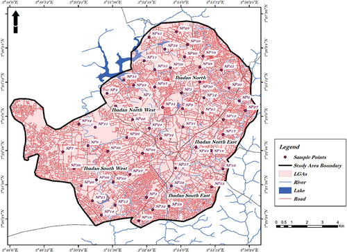
Ibadan (the capital of Oyo State, Nigeria) is located in the heart of Southwest Nigeria, and with respect to the geographical area, it is the largest city In Nigeria (Figure 1). Ibadan has an alternating wet, of up to 8 months, and dry, of about 4 months, seasons with relatively constant atmospheric temperature per annum. The mean maximum temperature of Ibadan is about 26.46°C, the mean minimum temperature of 21.42°C, and relative humidity of 74.55% (Amanambu, 2015). The month of June has the highest record of mean monthly rainfall of approximately 125 mm, with January having the lowest of approximately 18 mm. The mean annual rainfall is about 1205 mm, which falls for about 3 months and 19 days, having two peaks in June and September (Egbinola & Amanambu, 2014). A total of 60 sampling points were selected to cut across the identified land use activities in the study area.

Figure 1. Map of Ibadan Metropolis showing sample points.

1.1.2. Geology

The study site is underlain by a basement complex, characterized by igneous and metamorphic rocks of the Precambrian era. Granite quartzite and migmatite are the major rock types (Egbinola & Amanambu, 2014). Usually, the rock types found within this area are regarded as poor aquifers, given their low permeability and porosity (Amanambu, 2015; Egbinola & Amanambu, 2014). Though, some levels of porosity and permeability are developed through fractures and weathering, which in turn depends on the parent material. Therefore, the accessibility of groundwater depends on the weathered material’s level and the extent to which joints and fractures are present (Egbinola & Amanambu, 2014).

1.2. Materials and methods

1.2.1. Sampling

The sampling area is the metropolitan area of Ibadan consisting of five local government areas, Ibadan North, Ibadan North east, Ibadan North west, Ibadan South East and Ibadan South west. (Figure 1). This research required mainly data on the groundwater quality parameters. To assess the level of groundwater contamination, sampling of groundwater was done from hand dug wells located in the study area across the identified land use or prevalent anthropogenic activity. These include; Residential, Commercial, Industrial, Educational, and Agricultural areas. Furthermore, prevalent factors of possible contamination were identified in this area and were categorized broadly as follows: use of pesticides & herbicides, fertilizers, septic discharge, leachates from landfill and dumpsites, effluents and industrial wastes.

Good quality narrow mouth screw-capped polypropylene bottles of two-liter capacity were utilized in collection of the water sample. Bottles were pre-washed with dilute nitric acid, and rinsed with DM (Demineralized) water afterward to ensure that collected samples are not tainted by pre-existing water or impurities in the bottles. The groundwater samples retrieved in a prewashed polyethylene bottles were analyzed for the following parameters; pH, E.C, and TDS were taken onsite with the aid of a multi-parameter water meter. The concentrations of Calcium (Ca+) and Magnesium (Mg+) were measured by the volumetric method in the presence of an aqueous EDTA solution; this method was also used for titration of carbonates (HCO₃). Chloride (Cl⁻) was determined in the neutral medium by a titrated solution of silver nitrate in the presence of potassium chromate. The measurement of nitrates (NO₃⁻) and sulphate (SO₄²⁻) was carried out by a spectrophotometric method (Bashir et al., 2020), and that potassium (K⁺) and sodium (Na+) was determined by a flame photometer (Bouteraa, Mebarki, Bouaicha, Nouaceur, & Laignel, 2019). The coordinates of the sample points in the study area were obtained using a global positioning system (GPS) device, and then inputted into the ArcGIS environment in generating a map of the study area showing the sample points (Thomas, 2023). These coordinates were also utilized in the spatial analysis model employed.

1.2.2. Techniques

Hierarchical Cluster Analysis (HCA) is a valuable data classification technique used to categorize groundwater samples in Q-mode HCA or physicochemical indices in R-mode HCA. This analysis enables the identification of independent clusters, providing insights into the factors that influence groundwater chemistry (Wu, Li, Wang, Ren, & Wei, 2019). The Ward’s linkage method, proposed by Ward in 1963, was employed for this purpose. The analysis was performed on normalized data, using the squared Euclidean distances as a measure of similarity (Venkatramanan, Chung, Kim, Kim, & Selvam, 2016). The Ward’s linkage method is a powerful grouping mechanism that utilizes an analysis of variance approach to evaluate the distances between clusters (Das, Mondal, Ghosh, & Sutradhar, 2019). Its objective is to minimize the sum of squares of any clusters that can be formed at each step of the analysis. To ensure the reliability and comparability of the data, standardization was applied to the sample data. This standardization is necessary because different components of water quality may have varying units. By standardizing the data, each variable carries equal weight and influence in the analysis, facilitating accurate comparisons and interpretations of the results (Dhakate, Mahesh, Sankaran, & Gurundha Rao, 2013).

In order to conduct accurate hydro-chemical analysis of groundwater data, the technique of principal component analysis (PCA) was utilized to effectively reduce the dimensionality of the dataset (Ahamed, Loganathan, Ananthakrishnan, Ahmed, & Ashraf, 2017; Grande, González, Beltrán, & Sánchez-Rodas, 1996; Thapa, Gupta, & Reddy, 2017). The computation of Principal Component Analysis (PCA) was performed using IBM SPSS statistical software version 20. PCA effectively captures essential insights into the components of extensive datasets while minimizing information loss. The analyzed groundwater samples were subjected to Principal component analysis (PCA) in order to acquire an overall idea about assembling the samples in a multidimensional space specified by the assessed parameters. Principal component analysis is a valuable approach for gaining a better understanding of the connection between variables and identifying groupings (or clusters) that are mutually associated within a data body. PCA is expressed mathematically as follows:

(1) $Z_1=a_1{x}_1+a_2{x}_2+...+a_n{x}_n$(1)

where Z₁ is the first principal component, x₁, x₂, … , x_n are the original variables (e.g. PH, EC, Ca, Mg, Na, etc.) and a₁, a₂, … a_n are the coefficient or weight of each variable for the first principal component Z_1.

By combining HCA and PCA, a comprehensive understanding of groundwater chemistry can be achieved, shedding light on the underlying factors that shape its characteristics and behavior.

1.2.3. Kruskal–Wallis test

The Kruskal–Wallis test was employed to examine the variation of the concentration level of the selected water quality parameters. It is used for comparing more than two independent samples of same of different sample sizes (Kruskal & Wallis, 1952). It is expressed mathematically as:

(2) $\text{{bf{it{H}}} = left({{bf{it{N}}} - 1} right){{mathop sum limits^ \_{{{it{g}}}}\_{{bf{it{i}}} = 1}{{bf{it{n}}}\_{bf{it{i}}}}{{left({acute{{{bf{it{r}}}\_{{{i}}}}} - {{{acute r}}}} right)}^2}} over {mathop sum limits^ {{{it{g}}}}\_\_{{bf{it{i}}} = 1}mathop sum limits^ {{{{it{n}}}\_{{it{i}}}}}\_{{bf{it{j}}} = 1}{{left({{{bf{it{r}}}\_{{bf{it{ij}}}}} - {{{acute r}}}} right)}^2}}}}$(2)

Where:

N = total number of observations across all groups

G = number of groups

n_i = number of observations in group i

r_ij = rank of observations j from group i

${\acute{r}}_{i.}=\hspace{0.17em}\frac{\sum _{j=1}^{n_i}{r}_{ij}}{n_i}$ is the average rank of all observations in group i

$\acute{r}=\hspace{0.17em}\frac{1}{2}\hspace{0.17em}\left(N+1\right)$ is the average of all the r_ij

1.2.4. Correlation analysis

This is a quantification of the connection between two variables. It shows the direction of relationship (positive or negative) and the extent of the relationship (weak or strong) (Pearson, 1904). These methods generate values that indicate the direction of the relationship between variables as well as the extent of the relationship. A correlation coefficient of zero (0) implies that the two variables being observed are not related or no association exists between them, while a correlation coefficient value of 1 implies that the variables being measured are perfectly related (Metsamuuronen, 2022; Thapa, Gupta, & Reddy, 2017). It is also noteworthy that the correlation or association between two variables can neither be lesser nor greater than 1. Correlation matrix of Karl Pearson has been prepared to present the association between individual parameters of groundwater chemical and to identify the link between them (Egbueri, Mgbenu, & Chukwu, 2019; Loganathan & Ahamed, 2017; Wenning & Erickson, 1994). The correlation value of > .05 represents very high correlation between variables, <.05 demarcated poor correlation between variables and .05 value of correlation represents moderate relationship between variables (Das, Mondal, Ghosh, & Sutradhar, 2019). The Pearson product-moment correlation (PPMC) coefficient statistics, is also referred to as the Bivariate correlation and denoted by r is obtained by substituting values into the formula shown below;

$\text{r={frac{Sigmaleft(u-{bar u}right)left(y\_i- {bar y}}right)}over{sqrt{Sigmaleft(u-{bar u}right)^2}sqrtSigmaleft(y\_i-{bar y}right)^2}}}$

where r = Pearson coefficient

u_i = values of u-variable in the sample

Ū = average values of the u-variables

y_i = values of y-variable in the sample

Ӯ = average value of the y-variables

Also, for PPMCC, −1 ≤ r ≤ +1 implying that the correlation coefficient can neither be lesser nor greater than 1. This was utilized to scrutinize the relationship between the climatic data and the concentration level of the geogenic contaminants in the study area.

1.2.5. Groundwater quality index (GWQI)

This index gives an unbiased evaluation of water quality by taking into account all of the factors evaluated for each water sample. The Ground Water Quality Index (GWQI) is a relatively new tool for determining groundwater quality at a glimpse. In the current investigation, the GWQI calculations for each sampling point required three phases (Li et al., 2011). The first phase was “weight assignment,” where each of the parameters that were allocated weights (W_i), based on their respective relevance in terms of overall drinking water quality. The most important characteristics were assigned a weight of 5, while the least significant were assigned a weight of 1 (Mahmud, Sikder, & Joardar, 2020).

The next stage will be to compute relative weights for each water quality characteristic. The relative weight (W_i) was computed using Equation 1(1) $Z_1=a_1{x}_1+a_2{x}_2+...+a_n{x}_n$(1) as pointed out by (Mahmud, Sikder, & Joardar, 2020).

(3) $W_i=\frac{w_i}{{\mathrm{\Sigma }}_{i=1}^n{w}_i},$(3)

where: W_i is the relative weight, w_i is the weight of each parameter, and n is the number of parameters.

The next step was to calculate the quality rating scale. The quality rating scale (q_i) for each parameter was calculated using Equation 2(2) $\text{{bf{it{H}}} = left({{bf{it{N}}} - 1} right){{mathop sum limits^ \_{{{it{g}}}}\_{{bf{it{i}}} = 1}{{bf{it{n}}}\_{bf{it{i}}}}{{left({acute{{{bf{it{r}}}\_{{{i}}}}} - {{{acute r}}}} right)}^2}} over {mathop sum limits^ {{{it{g}}}}\_\_{{bf{it{i}}} = 1}mathop sum limits^ {{{{it{n}}}\_{{it{i}}}}}\_{{bf{it{j}}} = 1}{{left({{{bf{it{r}}}\_{{bf{it{ij}}}}} - {{{acute r}}}} right)}^2}}}}$(2) (Iwar, Ogedengbe, Katibi, & Jabbo, 2021):

(4) $qi=\hspace{0.17em}\frac{C_i}{S_i\hspace{0.17em}}\ast 100,$(4)

where, qi is the quality rating, C_i is the concentration of each chemical parameter in each water sample in mg/L, except pH and E.C, and S_i is the WHO standard for each chemical parameter.

Finally, the W_i and q_i were used to compute the SI_i for each chemical parameter (Equation. 3(3) $W_i=\frac{w_i}{{\mathrm{\Sigma }}_{i=1}^n{w}_i},$(3) ), and then the WQI was calculated using Equation 4.(4) $qi=\hspace{0.17em}\frac{C_i}{S_i\hspace{0.17em}}\ast 100,$(4)

(5) $S{I}_i=W_i\ast qi$(5)

(6) $WQI=\hspace{0.17em}\sum _{i=1}^{n}S{I}_i$(6)

where, SI_i is the sub-index of each parameter, qi is the rating based on concentration of each parameter, and n is the number of parameters.” Furthermore, the Inverse Distant weight interpolation in ArcGIS was employed to depict the spatial distribution of the GWQI.

1.3. Results and discussion

The difference in the concentration levels of the examined water quality parameters of the study area across sixty (60) sample points was investigated for inherent differences with respect to the prevalent human activity around the sample points. Nine main lithological classes were identified in the study area; garnel amphibolite, augen gneiss, biotite gneiss, gneiss, granite, granite gneiss, pegmatite quartz and quartz-vein. Pearson correlation statistical technique was employed to investigate the relationship between the water quality parameters. Hierarchical Cluster Analysis (HCA) was used to categorize groundwater samples into sample point across lithology and physicochemical indices. Principal Component Analysis technique was used to examine the relationship in concentration levels of groundwater parameters and to ascertain the presence of any form of influence of the underlying lithology on the concentration levels. Principal Component Analysis technique was also employed used to examine the relationship between prevalent anthropogenic factor and the concentration levels of water quality parameters. Five prevalent anthropogenic factors were identified in the field from the dominant land uses adjoining the sample points, and this were employed to examine which of these factors exerts the most influence on the concentration levels of parameters.

1.3.1. Lithological influence on groundwater hydrochemistry

The R mode HCA clusters the physicochemical data into several groups. Based on the Figure 2, three main clusters can be identified among lithological class variables labeled 1, 2, and 3, respectively. The first cluster is also divided into two sub-divisions; the first sub-cluster within cluster two consists of NO₃⁻, SO₄^2-, Ca²⁺, Mg²⁺, and pH. The second sub-cluster within the second cluster division consists of Na⁺ and K⁺. The second cluster is further sub-divided into two clusters, the first sub-cluster consists of TDS alone, while the second sub-cluster within cluster one consists of carbonates (HCO₃⁻) and Cl⁻. The third cluster identified consist of E.C only.

Figure 2. R mode Dendrogram of HCA of groundwater physicochemical variables.

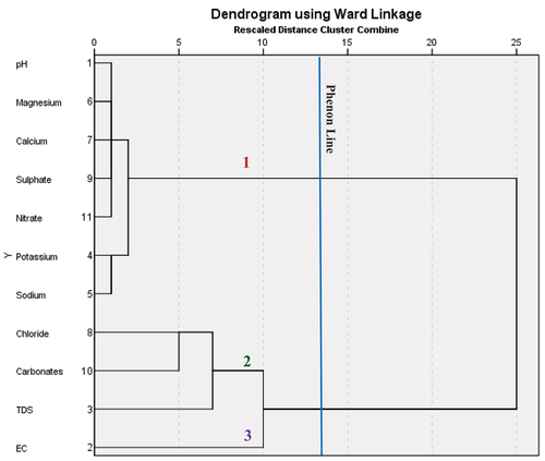
The first sub-cluster of the of the first main cluster is likely from natural processes, whereas the second subcluster of this category may be attributed by anthropogenic sources such as agricultural practices, sewage activities, and wastewater and effluents from industries. The second and third main clusters can be inferred to be affected mainly by mineral dissolution and second cluster be attributed by multiple factor; there are many processes that influencing the geochemistry of groundwater. Cl⁻ in the first sub-cluster represents flushing of evaporated minerals from sedimentary influence.

The Q mode HCA clusters the sampling point data into groups based on the lithological class in Figure 3. Observation of the Q mode HCA dendrogram reveals that the three clusters have distinctive lithological characteristics. Based on the Figure 3, two main clusters can be identified among lithological class variables labeled Clusters 1, 2, and 3, respectively. Cluster 1 includes 19 groundwater samples, and is further sub-divided into two sub-clusters, the first sub-cluster is further divided into two subdivisions; the first subdivision consists of points 27, 51, 42, 55, 38, and 56; while the second subdivision of the first sub-cluster consists of 34, 44, 43, 45, 35, 50, and 29, showing the highest mean concentration of NO₃⁻, SO₄^2-, Ca²⁺, Mg²⁺. The second sub-cluster of Cluster 1 is also divided into two, the first subdivision consists of points 39, 47, 41, 52, and 37; while the second subdivision of the first sub-cluster consists of only point 40, showing the highest mean concentration of Na⁺ and K⁺. This cluster is mainly dominated by the following lithological classes; biotite-gneiss, Pegmatite, Granite gneiss, Quartz-vein, and Gneiss, and further suggesting the strongest natural mineral dissolution processes and a few anthropogenic contaminations of groundwater across those sample points.

Figure 3. Q mode dendrogram of HCA of Lithological Class of sample points.

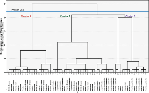
Cluster 2 includes 27 groundwater samples, and is further sub-divided into two sub-clusters, the first consists of points 10, 11, 12, 7, and 14. The second sub-cluster is further divided into two subdivisions; the first subdivision was further divided into two subdivisions which consists of four points (22, 46, 4, and 6), and 10 points (32, 59, 30, 28, 53, 31, 60, 48, 49, and 54), respectively, these cluster show the highest mean concentration of carbonates (HCO₃⁻), and Cl⁻. The second subdivision of the second sub-cluster consists of two subdivisions as well which consists two points (9 and 57) and six points (8, 19, 16, 17, 3, and 5) these cluster show the highest mean concentration of TDS (Das & Nag, 2017). This cluster is mainly dominated by the following lithological classes; augen-gneiss, garnel-amphibolite, quartz, pegmatite, granite-gneiss, quartz-vein, and biotite-gneiss suggesting dissolution of minerals of metamorphic origin and a great degree of mineralization which may be attributed to both natural and anthropogenic origin.

Finally, cluster 3 includes 14 groundwater samples, and is further sub-divided into two sub-clusters, the first consists of points 20, 21, and 23. The second sub-cluster is further divided into two subdivisions; the first subdivision was further divided into two subdivisions which consists of four points (33, 58, 36, and 26), and seven points (2, 24, 1, 13, 15, 25, and 18), respectively. These cluster and its subclusters show the highest mean concentration of E.C (Bouteraa, Mebarki, Bouaicha, Nouaceur, & Laignel, 2019). This cluster is mainly dominated by the following lithological classes; garnel-amphibolite, quartz, gneiss, quartz-vein, granite, and biotite-gneiss suggesting high mineral dissolution either of natural or anthropogenic origin (Egbueri, Mgbenu, & Chukwu, 2019). The natural origin is indicative of the dissolution of minerals such as salts, carbonates, and sulfates; which may have originate from geological formations through the weathering and leaching of rocks and minerals. The anthropogenic origin may be attributed to introduction of pollutants and elevated levels of ions and chemicals from industrial effluents, runoff from agricultural fields, and improper waste disposal can into groundwater.

1.3.2. Correlation analysis

Pearson correlation analysis was carried out on 60 samples with 11 physicochemical parameters each, and the correlation coefficient matrix is shown in Table 1. pH is significantly correlated with Na⁺ and Ca²⁺, with corresponding positive correlation coefficients of 0.480 and 0.257, while pH was negatively correlated with Cl⁻ and HCO₃⁻ , with negative correlation coefficients of −416 and −0.398, which indicates that any concentration fluctuations in pH levels, there is a counter effect on chloride and carbonates in the opposite direction. In other words, the more alkaline the pH is, the lower the chloride and carbonate levels, and vice-versa. TDS levels were significantly positively correlated with K⁺ concentration levels with a correlation coefficient of 0.228.

Table 1. Correlation Matrix.

	pH	EC	TDS	K^+	Na^+	Mg^2+	Ca^2+	Cl^−	HCO3^−	SO4^−	NO3^−
pH	1
EC	.086	1
	.511
TDS	.212	.097	1
	.100	.457
K^+	.060	.213	.288	1
	.646	.099	.024
Na^+	.480	−.004	.194	−.049	1
	.000	.977	.133	.708
Mg^2+	.191	−.180	−.040	−.220	.771	1
	.140	.165	.758	.088	.000
Ca^2+	.257	−.195	−.025	−.226	.849	.968	1
	.045	.132	.850	.081	.000	.000
Cl^−	−.416	.095	−.076	.111	−.320*	−.073	−.095	1
	.001	.468	.558	.395	.012	.576	.466
HCO3^−	−.398	−.146	−.217	−.082	−.248	.030	−.009	.302	1
	.002	.261	.093	.532	.054	.816	.942	.018
SO4^−	.178	.055	−.091	−.134	.128	−.174	.125	−.182	−.218	1
	.172	.674	.489	.307	.331	.185	.340	.164	.094
NO3^−	.092	−.026	−.079	−.023	.011	.017	.127	−.177	−.289	.244	1
	.484	.847	.551	.864	.934	.899	.335	.177	.025	.060

Furthermore, Na⁺ was observed to be statistically significantly correlated with Ca²⁺ and Mg²⁺ with correlation coefficients given as, 0.849 and 0.968, which indicate strong correlation. In other words, the presence of sodium at a sample point or well, informs the presence of calcium and magnesium. This implies that the underlying lithology from which dissolution of minerals occur are likely of the class (Li et al., 2018; Pophare, Balpande, & Nawale, 2018). On the one hand, that Cl⁻ was observed to exhibit a strong positive correlation with the presence of HCO₃⁻, with a correlation coefficient of 0.302, while on the other hand, HCO₃⁻ is also negatively significantly correlated with NO₃ with correlation coefficient of −0.289. This implies that both parameters are in opposite direction connoting that any fluctuation or flux in one will result in the alteration in the concentration level of the other. It is logical to infer that the dissolution of chemicals of anthropogenic origin having accumulated over time, might be responsible for these levels of chloride and carbonates. Higher HCO₃ content may promote higher alkalinity level, which may consequently affect human health. This correlates with findings of Wu, Li, Wang, Ren, and Wei (2019) and (Das, Mondal, Ghosh, & Sutradhar, 2019).

1.3.3. Multivariate statistical techniques

1.3.3.1. Kaiser–Maiyer–Olkin (KMO) and bartlett sphericity

All samples were subjected to PCA analysis, which revealed a 0.558 value for the Kaiser–Maiyer–Olkin (KMO) and a value of 129.697 (p 0.000) for Bartlett’s sphericity (Table 2), indicating that PCA was effective in giving significant reductions in dimensionality.

Table 2. KMO and Bartlett Result.

Kaiser–Meyer–Olkin Measure of Sampling Adequacy.		.558
Bartlett’s Test of Sphericity	Approx. Chi-Square	129.697
	df	55
	Sig.	.000

1.3.3.2. Communalities

In explaining the proportion of variables that are explainable by the underlying lithology which in this case are the principal components, the principal component analysis gave the proportion of variance of the variables (Table 3), to depict the amount of influence the underlying lithology has on the concentration level of water quality parameter. To this end, this analysis explains how much of the observed concentration levels of the selected water quality parameter is explainable by the lithological classes across the study area. This proportion is observable from the extent by which the extraction values deviate from the Initial values which is usually denoted as 1. Firstly, the PCs were discovered to only account for 58.7% and 56% of the factors that influence pH and TDS levels of groundwater in the study area. The PCs account for 60%, 62.3%, and 67.2% of the factors that influence the concentration levels of SO₄⁻, HCO₃⁻, and NO₃⁻ observed in the study area. Next the PCs account for 70.6%, 72.7%, 75.5%, 77.3%, of the factor responsible for the observed concentration levels of Cl⁻, K⁺, E.C, and Mg²⁺. Finally, the PCs accounted for 81.3% and 87.2% of the factors that appeared to have exerted influence on the recorded concentration levels of Na⁺ and Ca²⁺.

Table 3. Explainable variance by PCs.

Parameters	Initial	Extraction	Extraction (%)
pH	1.000	.587	58.7
EC	1.000	.755	75.5
TDS	1.000	.560	56.0
Potassium	1.000	.727	72.7
Sodium	1.000	.813	81.3
Magnesium	1.000	.773	77.3
Calcium	1.000	.872	87.2
Chloride	1.000	.706	70.6
Carbonates	1.000	.623	62.3
Sulphates	1.000	.600	60.0
Nitrates	1.000	.672	67.2

1.3.3.3. Principal component analysis

From the result of the PCA (Table 4), pH, Na⁺, and TDS marked component 1, which explained 25.543% of the total variance. Factor 1 had a high positive loading on pH (0.735), Na⁺ (0.855), and TDS (0.429), respectively. High positive loadings indicated strong linear correlation between the factor and parameters. The class of highly mineralized lithology can be marked as factor 1 which exerts influence on the amount of TDS found in the water samples. Factor 2, with higher positive loading of K⁺ and partly TDS explained 14.657% of variance with loading of 0.610 and 0.551, respectively. Component 2 in agreement with factor one is premised on the nature of the underlying rock within the study area, in other words, the levels of potassium and TDS can be accrued to the dissolution of rock minerals through regular interaction of rock and water. Component 3 accounted for 10.404% of total variance and best mainly represented by Calcium 0.706. Groundwater of high TDS value encourages the mobilization of compound contaminants such as carbonates, and nitrates. This single fact confirms the relationship between TDS and other compound contaminants. Leaching through downward washing of dissolved minerals through the soil profile can increase the calcium of the groundwater and the process is evidenced in higher TDS values. Dissolved solids produce hard water, which leaves deposits and films on fixtures, and on the insides of hot water pipes and boilers. Soaps and detergents do not produce as much lather with hard water as with soft water. As well as this, high amounts of dissolved solids can stain household fixtures, corrode pipes, and have a metallic taste. Component 4 was responsible for 10.092 % of total variance and partly represented by potassium; 0.504 and calcium; 0.527. Groundwater of high sodium value is probably indicative of natural occurrence. This is an indication that groundwater with high levels of dissolved inorganic salts must have originated from water that has flowed through a region where the rocks have a high salt content (Amanambu, 2015). Groundwater of high calcium value encourages the higher dissolution of solids leading to hardness of water. The human body needs calcium for strong teeth and bones. Finally, component 5 accounted for 9.198% of the total variance and is represented by E.C (0.584) and chloride (0.488), in agreement with the findings of Amanambu (2015).

Table 4. Loading matrix of principal components and variance of explanation.

Parameters	Components
	1	2	3	4	5
pH	.735	−.007	−.088	−.193	−.043
EC	.271	.365	−.298	.345	.584
TDS	.429	.551	−.068	−.146	−.215
Potassium	.257	.610	.067	.504	−.175
Sodium	.855	.204	.199	−.016	.014
Magnesium	−.471	.089	−.496	.370	−.401
Calcium	.196	−.208	.706	.527	−.114
Chloride	−.572	.340	.056	.145	.488
Carbonates	−.680	.112	.384	.013	−.024
Sulphates	.330	−.558	−.049	.143	.395
Nitrates	.235	−.520	−.319	.471	−.150
Total	2.810	1.612	1.144	1.110	1.012
% of Variance	25.543	14.657	10.404	10.092	9.198
Cumulative %	25.543	40.200	50.604	60.696	69.894

1.3.3.4. Scree plot

A Scree plot is a basic linear graph that illustrates the proportion of total variation explained or represented by each element in the data. The factors are arranged, and therefore given a number label, in decreasing order of contribution to total variance. A scree plot is a graph of eigenvalues in ascending order of magnitude. It demonstrates a clear distinction between the slope angle of the strong eigenvalues and the progressive falling off of the remaining components. The five extracted components (eigenvalues >1) appropriately represented the aggregate dimensions of the data set and compensated for 69.894% of the total variance in the current research, whereas the other six factors (eigenvalues <1) accounted for just 30.106% of the total variance (Figure 4).

Figure 4. Scree Plot of Component Loading.

1.4. Groundwater hydrochemistry, land use and permissible limits

1.4.1. Variation in groundwater hydrochemistry across anthropogenic activity

Five main human activities were identified in the field reflective of the dominant land uses identified in the study area; pesticides and herbicides, fertilizers, septic discharge, landfill and dumpsite, and industrial effluents and discharge. The difference in the concentration levels of the examined water quality parameters of the study area across sixty (60) sample points was investigated for inherent relationship with respect to the prevalent anthropogenic activity around the sample points. The Kruskal–Wallis statistical technique was used to examine these in concentration levels of groundwater parameters and to ascertain the presence of any form of influence of the prevalent anthropogenic activity on the concentration levels.

From Table 5, the Kruskal–Wallis test ranked the factor with respect to their relative impact on the respective parameters. This made it possible to identify the factor that contributed the most to the concentration level of the water quality parameters in the study area. With respect to pH, the use of fertilizers emerged as the major factor influencing pH level in the study area (mean rank of = 52.8), this implies that over time leachates of fertilizers have been washed down the soil profile to impact the contamination of the groundwater. Next to this is seepage from landfill and dumpsite (mean rank = 31.9), and third is septic discharge and seepage (mean rank = 31.2). These three factors exert greater influence on the pH levels of groundwater across the study area.

Table 5. Mean effect ranking of anthropogenic activity.

Factor	pH	EC	TDS	K^+	Na^+	Mg^2+	Ca^2+	Cl^−	HCO3^−	SO4^−	NO3^−
Use of pesticides & herbicides	29.2	26.6	23.0	28.3	27.6	31.3	32.4	26.4	33.7	28.1	31.9
Fertilizers	52.8	44.8	38.0	41.5	43.5	26.1	35.3	14.4	19.8	37.8	16.8
Septic discharge and seepage	31.2	27.4	29.5	29.1	29.3	26.4	32.3	32.0	31.0	27.2	32.5
Landfill and dumpsites	31.9	23.8	41.6	28.4	39.1	26.7	21.1	28.7	23.0	40.4	32.7
Industrial effluents and waste	12.8	42.3	32.1	32.4	22.2	47.9	26.3	47.3	37.4	30.7	30.3

Furthermore, fertilizer application also exerted the dominant influence on E.C (mean rank = 44.8). This may probably be alluded to the presence of potassium in the fertilizers been used. Second in this category is industrial effluents and waste (mean rank = 42.3). Fertilizer application was also the dominant factor affecting the concentration levels of K⁺, Na⁺, and Ca²⁺ with mean rank of effects as; 41.5, 43.5, 35.3, respectively, for each parameter, as pertaining to fertilizer application.

Land fill and dumpsites exerted more influence on the levels of TDS, SO₄⁻, and NO₃⁻ with mean ranks 41.6, 40.4, 32.7, respectively. Industrial effluents and wastes were found to exert the most dominance on the concentration levels of Mg²⁺, Cl⁻, and HCO₃⁻; with mean ranks of 47.9, 47.3, 37.4.

In Table 6, the Kruskal–Wallis test further examined the statistical significance of the power of the mean ranking of effects. The result (Table 6) revealed that pH, EC, Magnesium and Chloride, were significantly influenced by the prevailing factors across the study area. This was revealed by the p < 0.05. However, TDS, potassium, sodium, calcium, carbonates, sulphates, nitrates appeared not to have been significantly influenced by the prevalent anthropogenic activity across the study area. Albeit, if there any form of influences on these parameters exerted by the prevalent activities, it is not statistically significant

Table 6. Kruskal–Wallis test of prevailing factor.

Parameter	Chi-Square	p value	Remark
pH	18.479	.001	Significant
EC	10.251	.036	Significant
TDS	6.870	.143	Not Significant
K+	2.965	.564	Not Significant
Na+	7.372	.117	Not Significant
Mg2+	10.069	.039	Significant
Ca2+	3.363	.499	Not Significant
Cl-	13.600	.009	Significant
HCO3-	5.337	.254	Not Significant
SO4-	4.417	.353	Not Significant
NO3-	4.188	.381	Not Significant

1.4.2. Groundwater hydrochemistry and WHO standard

The concentration levels of parameters of water quality recorded from the laboratory analysis of the samples obtained from the study area were compared against the WHO permissible limit for drinking water. This was done to examine the potability of the water sample obtained across different sample points in the study area. Table 7 gives the permissible limits of hydrochemistry parameters for drinking water as recommended by the WHO against the mean observed concentration levels of parameters. However, the statistical analysis was carried by comparing the observed values of each sample point to the WHO standard.

Table 7. Guideline for potable water (WHO, and observed).

Parameter	Minimum	Maximum	Mean	Std. Deviation	WHO
pH	4.40	7.10	6.49	.49104	7.5
EC	270.00	1870.00	893.56	326.55731	400
TDS	142.00	1720.00	536.88	290.22752	500
K+	9.80	99.60	56.97	19.38374	20
Na+	5.10	59.52	31.96	13.94075	200
Mg2+	3.73	9.50	6.02	1.25199	50
Ca2+	1.30	7.37	4.71	1.33943	100
Cl-	57.60	1476.00	445.01	304.69540	250
SO4-	.00	6.10	2.26	1.30636	250
HCO3-	100.50	609.00	253.00	111.75046	240
NO3-	.00	6.09	1.36	.98732	50

Furthermore, a chart (Figure 5) was employed to examine the inherent differences between the observed values and the World Health Organization (WHO) standard. It can be observed that, on the overall, the observed EC, TDS, chloride and carbonates concentration levels were higher than the permissible limit of the WHO, while the remaining parameters; pH, Potassium, sodium, magnesium, calcium, sulphate, and nitrate were lower than the WHO limit with respect to concentration level.

Figure 5. Observed hydrochemistry levels and WHO limits.

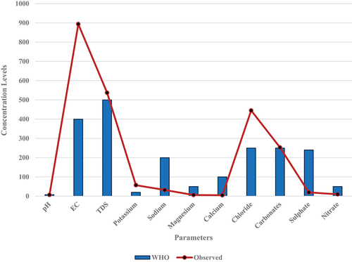
The Two samples”>independent or two samples “t” distribution test was employed to ascertain if there are statistically significant differences in the observed value of parameters recorded from field observation across the 60 sample points, and the WHO standard (Table 8). The analysis was conducted at a threshold of 95% confidence interval and a probability level of p ≤ 0.05. The result of the analysis is given in Table 8, which reveals that pH (Sig. = .021), EC (Sig. = .031), K⁺ (Sig. = .000), Na⁺ (Sig. = .000), Mg²⁺ (Sig. = .000), Ca²⁺ (Sig. = .000), HCO₃⁻ (Sig. = .000), and NO₃⁻ (Sig. = .000); all differ significantly from the WHO limits. On the other hand, TDS (Sig. = .928), Chloride (Sig. = .321), and Sulphates (Sig. = .761) all exhibited a non-statistically significant difference from the WHO limits.

Table 8. Statistical comparison between observed concentration levels and WHO standard.

Parameters	N	DoF		t	P value (2-tailed)	Remark
pH	60	59	−2.803		.021	Significant
EC	60	59	2.562		.031	Significant
TDS	60	59	.093		.928	Not Significant
K+	60	59	7.935		.000	Significant
Na+	60	59	−14.168		.000	Significant
Mg2+	60	59	−58.572		.000	Significant
Ca2+	60	59	−138.974		.000	Significant
Cl-	60	59	1.050		.321	Not Significant
HCO3-	60	59	.313		.761	Not Significant
SO4-	60	59	−41.943		.000	Significant
NO3-	60	59	−10.045		.000	Significant

Going further, the pH value of the water significantly differs from the WHO limits. pH plays a crucial role in the taste and acceptability of water for consumption. These observed deviations may affect the palatability of the water. The EC is an indicator of the water’s mineral content and salinity., and raised levels of EC suggest the presence of dissolved solids, which can affect the taste and potentially have health implications. The TDS value does not exhibit a statistically significant difference from the WHO limits, while it may represents the overall concentration of dissolved solids in water, it is important to monitor TDS levels to ensure water quality and taste.

The following ions K⁺, Na⁺, Mg^2+, Ca²⁺, HCO₃⁻, and NO₃⁻, all demonstrated a significant difference from the WHO limits. Elevated levels of these ions affect the water’s taste, odor, and potentially pose health risks upon consumption. It imperative to constantly engage in monitoring and control of these parameters to ensure water safety. It is still important to monitor the levels chloride and sulphates parameters, as high concentrations impact the taste of water and have health implications in certain cases. Hence, deviations from the WHO standard limits should not be great and remediation mechanics should be initiated for contaminated well irrespective of the degree of contamination.

1.5. Groundwater suitability

The mean of computed WQI values for each location was categorized (Table 9), and the detailed computations for the GWQI for each location and parameter is provided in the spatial distribution map of GWQI below (Al-Omran, Al-Barakah, Altuquq, Aly, & Nadeem, 2015; Bashir et al., 2020).

Table 9. Relative weights of parameters in the study area.

Parameters	WHO Standard	Unit Weight	Wi	Qi	WiQi
pH	7.5	0.1333	0.46	86.67	39.55
EC	400	0.0025	0.01	223.39	1.91
TDS	500	0.0020	0.01	107.38	0.74
K+	200	0.0050	0.02	15.98	0.27
Na+	50	0.0200	0.07	12.04	0.82
Mg2+	100	0.0100	0.03	4.71	0.16
Ca2+	250	0.0040	0.01	178.00	2.44
Cl-	12	0.0833	0.29	18.79	5.36
HCO3-	125	0.0080	0.03	202.40	5.54
SO4-	250	0.0040	0.01	7.87	0.11
NO3-	50	0.0200	0.07	19.32	1.32
Σ			1.00		58.23

Based on the total weight of the GWQI, the water in the research region falls into the good water category of the groundwater categorization (Table 10) (Sahu & Sikdar, 2008), indicating that the groundwater available in the region is suitable for consumption however doesn’t negate the fact that the quality can be improved to contain little of not contaminants or that the level of the contaminants be brought to the barest minimum even below the recognized standards (Belkhiri, Tiri, & Mouni, 2020).

Table 10. Classification of groundwater based on GWQI.

Range	Type of water
<50	Excellent
50–100.1	Good water
100–200.1	Poor Water
200–300.1	Very Poor Water
>300	Water Unsuitable for drinking purposes

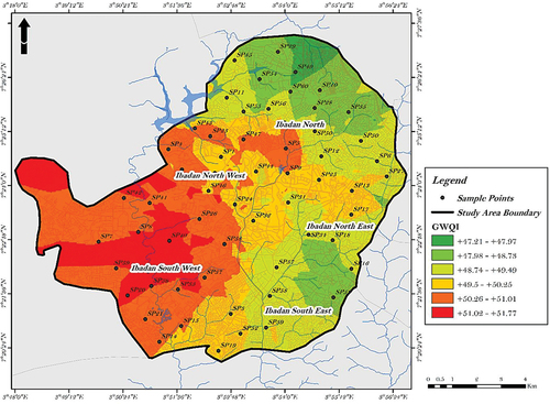
A spatial distribution of Groundwater Quality Index (GWQI) was mapped using the individual water quality index of the sample points (Figure 6). Analyzing the WQI values, we can categorize the sample points into two major water quality classifications. Points with a WQI below 50 falls into the “Excellent” category. These sample points represent excellent water quality in other words, the well or aquifer is not at risk of contamination. In the “Good water” category, which encompasses WQI values between 50 and 100.1, we find sample points that represent water with good quality, implying that the water in this well is at risk of being contaminated further, either by unchecked anthropogenic activities or effect of these activities.

Figure 6. Spatial Variation of GWQI across study area.

2. Conclusion

In conclusion, this research study has generated several significant findings. The application of multivariate statistics has proven effective in reducing the dimensionality of large datasets, allowing for the extraction of essential determinants for controlling groundwater quality. The analysis identified five components that collectively account for 69.9% of the total variance, highlighting their pivotal role as major factors influencing water quality. The study identifies that variations in groundwater quality parameters are primarily associated with natural water–rock interactions and anthropogenic influences. Moreover, the spatial analysis conducted through various statistical techniques assists in understanding the geographical distribution of key explanatory variables.

Furthermore, the use of statistical tools and graphical representation goes beyond basic research, as it facilitates the identification of regions with greater susceptibility to groundwater quality issues. This knowledge is crucial as it sheds light on potential negative impacts on human health and allows for appropriate interventions. The study’s assessment of groundwater quality using the Groundwater Quality Index (GWQI) revealed overall good drinking water quality throughout the study area, confirming the suitability of groundwater for human consumption.

This knowledge is invaluable for informed decision-making, benefiting environmentalists, hydrologists, and town planners. The findings support the optimization of groundwater quality, the sustainable management of groundwater resources, and the well-being of the general public. Importantly, the results of this study hold relevance for government and local authorities, providing them with valuable insights to inform policy and management strategies related to groundwater resources. By incorporating these findings into decision-making processes, steps can be taken to safeguard and improve groundwater quality, ensuring its long-term sustainability for the benefit of communities and the environment.

Disclosure statement

No potential conflict of interest was reported by the author.

References

- Ahamed, A. J., Loganathan, K., Ananthakrishnan, S., Ahmed, J. K. C., & Ashraf, M. A. (2017). Evaluation of graphical and multivariate statistical methods for classification and evaluation of groundwater in Alathur Block, Perambalur District, India. Applied Ecology and Environmental Sciences, 15, 105–116. https://doi.org/10.15666/aeer/1503_105116
- Al-Omran, A., Al-Barakah, F., Altuquq, A., Aly, A., & Nadeem, M. (2015). Drinking water quality assessment and water quality index of Riyadh, Saudi Arabia. Water Quality Research Journal of Canada, 50, 287–296. https://doi.org/10.2166/wqrjc.2015.039
- Amanambu, A. C. (2015). Geogenic contamination: Hydrogeochemical processes and relationships in shallow aquifers of Ibadan, South-West Nigeria. Bulletin of Geography Physical Geography Series, 9, 5–20. https://doi.org/10.1515/bgeo-2015-0011
- Bashir, N., Saeed, R., Afzaal, M., Ahmad, A., Muhammad, N. … Hameed, S. (2020). Water quality assessment of lower Jhelum canal in Pakistan by using geographic information system (GIS). Groundwater for Sustainable Development, 10. https://doi.org/10.1016/j.gsd.2020.100357
- Belkhiri, L., Tiri, A., & Mouni, L. (2020). Spatial distribution of the groundwater quality using kriging and Co-kriging interpolations. Groundwater for Sustainable Development, 11, 100473. https://doi.org/10.1016/j.gsd.2020.100473
- Bouteraa, O., Mebarki, A., Bouaicha, F., Nouaceur, Z., & Laignel, B. (2019). Groundwater quality assessment using multivariate analysis, geostatistical modeling, and water quality index (WQI): A case of study in the Boumerzoug-El Khroub valley of Northeast Algeria. Acta Geochimica, 38, 796–814. https://doi.org/10.1007/s11631-019-00329-x
- Das, N., Mondal, P., Ghosh, R., & Sutradhar, S. (2019). Groundwater quality assessment using multivariate statistical technique and hydro-chemical facies in Birbhum District, West Bengal, India. SN Applied Sciences, 1, 1–21. https://doi.org/10.1007/s42452-019-0841-5
- Das, S., & Nag, S. K. (2017). Application of multivariate statistical analysis concepts for assessment of hydrogeochemistry of groundwater — a study in Suri I and II blocks of Birbhum District, West Bengal, India. Applied Water Science, 7(2), 873–888. https://doi.org/10.1007/s13201-015-0299-6
- Dhakate, R., Mahesh, J., Sankaran, S., & Gurundha Rao, V. V. S. (2013). Multivariate statistical analysis for assessment of groundwater quality in talcher coalfield area, Odisha. Journal of the Geological Society of India, 82, 403–412. https://doi.org/10.1007/s12594-013-0167-7
- Díaz-Alcaide, S., & Martínez-Santos, P. (2019). Review: Advances in groundwater potential mapping. Hydrogeology Journal, 27, 2307–2324. https://doi.org/10.1007/s10040-019-02001-3
- Egbinola, C. N., & Amanambu, A. C. (2014). Groundwater contamination in Ibadan, South-West Nigeria. Springerplus, 3(1), 2–7. https://doi.org/10.1007/s10040-019-02001-3
- Egbueri, J. C., Mgbenu, C. N., & Chukwu, C. N. (2019). Investigating the hydrogeochemical processes and quality of water resources in Ojoto and environs using integrated classical methods. Modeling Earth Systems and Environment, 5, 1443–1461. https://doi.org/10.1007/s40808-019-00613-y
- Elubid, B. A., Huag, T., Ahmed, E. H., Zhao, J., Elhag, K. M., Abbass, W., & Babiker, M. M. (2019). Geospatial distributions of groundwater quality in Gedaref state using geographic information system (GIS) and drinking water quality index (DWQI). International Journal of Environmental Research and Public Health, 16, 1–20. https://doi.org/10.3390/ijerph16050731
- Emenike, C. P. G., Tenebe, I. T., & Jarvis, P. (2018). Fluoride contamination in groundwater sources in Southwestern Nigeria: Assessment using multivariate statistical approach and human health risk. Ecotoxicology and Environmental Safety, 156, 391–402. https://doi.org/10.1016/j.ecoenv.2018.03.022
- Grande, J. A., González, A., Beltrán, R., & Sánchez-Rodas, D. (1996). Application of factor analysis to the study of contamination in the aquifer system of ayamonte-huelva (Spain). Groundwater, 34, 155–161. https://doi.org/10.1111/j.1745-6584.1996.tb01875.x
- Iwar, R. T., Ogedengbe, K., Katibi, K. K., & Jabbo, J. N. (2021). Fluoride levels in deep aquifers of Makurdi, North-central, Nigeria: An appraisal based on multivariate statistics and human health risk analysis. Environmental Monitoring and Assessment, 193(8), 1–15. https://doi.org/10.1007/s10661-021-09230-8
- Kaur, T., Bhardwaj, R., & Arora, S. (2016). Assessment of groundwater quality for drinking and irrigation purposes using hydrochemical studies in Malwa region, southwestern part of Punjab, India. Applied Water Science, 7(6), 3301–3316. https://doi.org/10.1007/s13201-016-0476-2
- Kruskal, W. H., & Wallis, W. A. (1952). Use of ranks in one-criterion variance analysis William. Journal of the American Statistical Association, 47(260), 583–621. https://doi.org/10.1080/01621459.1952.10483441
- Li, M., Zhu, X., Zhu, F., Ren, G., Cao, G., & Song, L. (2011). Application of modified zeolite for ammonium removal from drinking water. Desalination, 271(1–3), 295–300. https://doi.org/10.1016/j.desal.2010.12.047
- Li, P., He, X., & Guo, W. (2019). Spatial groundwater quality and potential health risks due to nitrate ingestion through drinking water: A case study in Yan’an City on the Loess Plateau of northwest China. Human & Ecological Risk Assessment, 25(1–2), 11–31. https://doi.org/10.1080/10807039.2018.1553612
- Li, P., Wu, J., Tian, R., He, S., He, X., Xue, C., & Zhang, K. (2018). Geochemistry, hydraulic connectivity and quality appraisal of multilayered groundwater in the hongdunzi coal mine, Northwest. Mine Water and the Environment, 0, 0. https://doi.org/10.1007/s10230-017-0507-8
- Loganathan, K., & Ahamed, A. J. (2017). Multivariate statistical techniques for the evaluation of groundwater quality of Amaravathi River Basin: South India. Applied Water Science, 7(8), 4633–4649. https://doi.org/10.1007/s13201-017-0627-0
- Mahmud, A., Sikder, S., & Joardar, J. C. (2020). Assessment of groundwater quality in Khulna city of Bangladesh in terms of water quality index for drinking purpose. Applied Water Science, 10. https://doi.org/10.1007/s13201-020-01314-z
- Metsamuuronen, J. (2022). Reminder of the directional nature of the product–moment correlation coefficient, academia letters. Academia Letters. https://doi.org/10.20935/al5313
- Mohamed, M. M., & Elmahdy, S. I. (2015). Natural and anthropogenic factors affecting groundwater quality in the eastern region of the United Arab Emirates. Arabian Journal of Geosciences, 8, 7409–7423. https://doi.org/10.1007/s12517-014-1737-8
- Murphy, H. M., Prioleau, M. D., Borchardt, M. A., & Hynds, P. D. (2017). Review: Epidemiological evidence of groundwater contribution to global enteric disease, 1948–2015. Hydrogeology Journal, 25, 981–1001. https://doi.org/10.1007/s10040-017-1543-y
- Noshadi, M., & Ghafourian, A. (2016). Groundwater quality analysis using multivariate statistical techniques (case study: Fars province, Iran). Environmental Monitoring and Assessment, 188(7). https://doi.org/10.1007/s10661-016-5412-2
- Omo-Irabor, O. O., Olobaniyi, S. B., Oduyemi, K., & Akunna, J. (2008). Surface and groundwater water quality assessment using multivariate analytical methods: A case study of the Western Niger Delta, Nigeria. Physics and Chemistry of the Earth, 33, 666–673. https://doi.org/10.1016/j.pce.2008.06.019
- Pearson, K. (1904). Mathematical contributions to the theory of evolution XIII: On the theory of contingency and its relation to association and normal correlation (p. 46). 37 SOHO SQUARE, W., London: Drapers’ Company Research Memoirs: Biometric Series I. DULAU AND CO.
- Pophare, A. M., Balpande, U. S., & Nawale, V. P. (2018). Hydrochemistry of groundwater in Suketi river basin, Himachal Himalaya, India. Journal of Geosciences Research, 3, 67–83.
- Sahu, P., & Sikdar, P. K. (2008). Hydrochemical framework of the aquifer in and around East Kolkata Wetlands, West Bengal, India. Environmental Geology, 55, 823–835. https://doi.org/10.1007/s00254-007-1034-x
- Thapa, R., Gupta, S., & Reddy, D. V. (2017). Application of geospatial modelling technique in delineation of fluoride contamination zones within Dwarka Basin, Birbhum, India. Geoscience Frontiers, 8, 1105–1114. https://doi.org/10.1016/j.gsf.2016.11.006
- Thomas, E. O. (2021). Effect of temperature on D.O and T.D.S: A measure of Ground and Surface Water Interaction. Water Science, 35, 11–21. https://doi.org/10.1080/11104929.2020.1860276
- Thomas, E. O. (2023). Spatial evaluation of groundwater quality using factor analysis and geostatistical Kriging algorithm: A case study of Ibadan Metropolis, Nigeria. Water Practice & Technology, 18, 592–607. https://doi.org/10.2166/wpt.2023.023
- Venkatramanan, S., Chung, S. Y., Kim, T. H., Kim, B. W., & Selvam, S. (2016). Geostatistical techniques to evaluate groundwater contamination and its sources in Miryang City, Korea. Environmental Earth Sciences, 75(11). https://doi.org/10.1007/s12665-016-5813-0
- Viswanath, N. C., Kumar, P. G. D., Ammad, K. K., & Kumari, E. R. U. (2015). Ground water quality and multivariate statistical methods. Environmental Processes, 2, 347–360. https://doi.org/10.1007/s40710-015-0071-9
- Wenning, R. J., & Erickson, G. A. (1994). Interpretation and analysis of complex environmental data using chemometric methods. Trends in Analytical Chemistry, 13, 446–457. https://doi.org/10.1016/0165-9936(94)85026-7
- Wu, J., Li, P., Wang, D., Ren, X., & Wei, M. (2019). Human and ecological risk assessment: An international statistical and multivariate statistical techniques to trace the sources and affecting factors of groundwater pollution in a rapidly growing city on the Chinese Loess Plateau. Human and Ecological Risk Assessment, 0, 1–19. https://doi.org/10.1080/10807039.2019.1594156
- Xiao, Y., Shao, J., Frape, S. K., Cui, Y., Dang, X., Wang, S., & Ji, Y. (2018). Groundwater origin, flow regime and geochemical evolution in arid endorheic watersheds: A case study from the Qaidam Basin, northwestern China. Hydrology and Earth System Sciences, 22, 4381–4400. https://doi.org/10.5194/hess-22-4381-2018