Climate change in the upper Awash subbasin and its possible impacts on the stream flow, Oromiyaa, Ethiopia

ABSTRACT

Modelling climate change impact is very important to reduce the crisis behind food security, drought, and loss of energy sectors. The impact on streamflow and hydrological components due to climate change was aimed to investigate by the SWAT model for this study. Two regional climate models (RCM) were selected according to their performance to calibrate and validate the streamflow. The Regional Climate Models’ performance in simulation of flow and the hydrological cycle was evaluated by statistical performance criteria. Digital elevation model (DEM), land use land cover and soil map, and streamflow data were collected and used as raw input for the model. Bias correction was made by using power transformation and variance scaling method for RCM against observed data. The result simulated with RACMO22T was best with (PBIAS = 0.23, NSE = 0.84, R² = 0.79) for calibration, (PBIAS = 0.11, NSE = 0.88, R² = 0.81) for validation. RCA4 model underperformed in simulating streamflow compared to RACMO22T with (PBIAS = 0.28, NSE = 0.78, R² = 0.74) and (PBIAS = 0.18, NSE = 0.85, R² = 0.78) for calibration and validation of the models respectively. The streamflow was projected and shows a slightly increasing trend respectively with 13.8 and 21.3 % for the 2030s and 2050s simulation years. But in the 2080s simulation periods, the simulated streamflow indicates a decreasing trend under representative concentration pathways (RCP4.5) by 12.5%. The overall result indicates both streamflow and runoff show a decreasing pattern in the end of this century under both scenarios. The spatial variability of hydrological components which contributes to streamflow was dependent on the subbasin characteristics. Furthermore, the simulated groundwater recharge (GW_Q), rainfall, water yields (WYLD), surface runoff (SUR_Q) and evapotranspiration (ET) were decreased by 4%, 17.7%, 20.8%, 27.7%, and 8.6% respectively for the baseline period.

KEYWORDS:

• Bias correction
• climate change
• RCM
• spatial variability
• SWAT model

Introduction

There is no doubt that water is the most crucial resource by which every living thing is sustained over the Earth (Daba et al., 2011). However, in the 21^st century, in which the world has shown advancements in technology, and industrially civilized, emissions from industries sectors have brought climate change that exposes water resources to depletion (Chaemiso, Abebe, & Pingale, 2016). The majority of drought, shortage of energy sectors and instability of food security around the world have resulted from climate changes (Rojas-Downing et al., 2017). The impacts of climate change on the water resources of many river basins and catchments are increasing because of significant climate variability and increasing surface temperature (Bokke et al., 2017). The profound effect of climate variability on surface water resources remains a current focus on its sustainability for better mitigation through understanding the past and predicting its future consequences (Boko et al., 2020). In a river basins, hydrological extremes like baseflow, infiltration rate, groundwater, and surface runoff are affected by climate variability (Mahmoodi et al., 2021). Hence, flow parameters are very important in maintaining the hydrological cycles to determine the amount of evaporation, infiltration capacity, base-flows of rivers and surface runoff in the entire watershed (Zhang et al., 2016).

Regarding Ethiopia, the economic structure was highly dependent on traditional agriculture which is not easily flexible and adjustable to climate variability (Menna, 2017). The upper Awash subbasin is the most irrigable area in Ethiopia and by which many farmers take this basin as the guarantee of their food security (Daba & You, 2020). However, recently climate change has been highly ranked as the cause of the depletion of agricultural products and affecting many farmers and their economic productivity to be insufficient (Taye, 2018). The vulnerability aspect of river basins to climate change impact both in magnitude and direction mostly depends on the regional climate model, basins extent and hydrological models applied in the study (Y. Zhang et al., 2016). Meanwhile, new regional climate models (RCMs) lead to another opportunity, for the scientists to analyze the effects of climate change considering their higher spatial resolution and further reliable outcomes on a regional scale than general circulation models (GCMs) (Kang, Gao, Shao, & Zhang, 2020). Moreover, recent studies show pieces of evidence, that coordinated regional downscaling experiments (CORDEX) models and hydrological models are very crucial and more impactful in modeling hydrological variables (Yesuf et al., 2016). The main novelty of this study is an incorporation of two RCMs out of four applied according to their performance and setup SWAT model separately to realize the efficiency of both RCM and SWAT model to simulate rainfall, groundwater, percolation, lateral flow, potential evapotranspiration (PET), evapotranspiration (ET) and streamflow. But to analyze the impact of climate change on these hydrological cycles, the result obtained from an extreme scenario RCP8.5 was used to indicate hydro-meteorological trends (Mart et al., 2021). IPCC described RCP4.5 as a moderate scenario in which emission peak by 2040 and then declined, while RCP8.5 has been described as a worst scenario in which emission continue to rise throughout the 21^st century. Furthermore, many studies have used one RCM to set up the hydrological model to analyze the output using statistical parameters (Babar & Ramesh, 2013). But this study uniquely included statistical parameters that can evaluate the relationship of the simulated and observed by coefficient of determination (R2), Nash – Sutcliffe model efficiency coefficient (NSE), Correlation coefficient, root mean square error (RMSE), mean absolute error (MAE), an empirical formula that considers basin area, slope and annual precipitations, and other effective statistical properties such as$p\mathrm{\_}value$, coefficient of variations (CV), kurtosis and Skewness, Mean and Confidence intervals (CI). These parameters have been used to realize the fitness of simulated streamflow by the SWAT model against the recorded.

Materials and methods

Study area

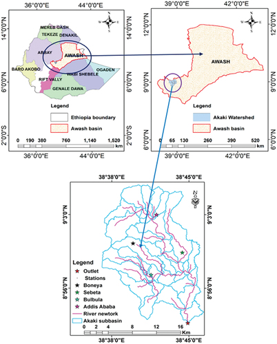
Akaki River is in the upper Awash subbasin and had a great contribution directly to Abba Samuel reservoir for electric power generation. The catchment was laid between 8°73” to 9° 25’N, latitude, and 38°62” to 39°12’E, longitudinal and has an area of 978.41 km² as shown in (Figure 1). The watershed has a subtropical highland climate with the lowest temperature in the study area was 7°C, which is in November and December, and the highest temperature was 28 °C in March and May (Brhane, Raba, Beketie, Feyisa, & Siyoum, 2022; Negash, 2023). The crucial recharge season that feeds the basin is from June to early September (Tumsa, 2022). The area receives 1,965 mm/year average annual rainfall and dry season starts in December through February (Zeberie, 2019).

Figure 1. Map of the study area.

Materials and its sources

Meteorological and spatial data

The SWAT model necessarily uses meteorological data such as precipitation, maximum and minimum temperatures, relative humidity, and wind speed for hydrological model development, future projection and to remove biases from RCM models in order not to mislead the desired results (Abdulahi, Abate, Harka, & Husen, 2022; Daba & You, 2020; Duguma, Feyessa, & Demissie, 2021; Emiru et al., 2022). All necessary data required for the model input is depicted in Table 1 below.

Table 1. Meteorological and spatial data used as an input for the SWAT model.

Data types	Stations	Length of record	Source of data
Meteorological data	Addis Ababa	1980 – 2005	National Meteorological Agency (NMA)
	Boneya
	Bulbula
	Sebeta
LULC and Soil map		2013	Ministry of Water, Irrigation and Electricity (MWIE)
DEM (12.5 by 12.5m)			http://vertex.daac.asf.alaska.edu

Hydrological data

Hydrological data was required to set up SWAT CUP to calibrate and validate streamflow under the two selected RCM models. The main gauging stations were along the river basin inside the catchment, which has a continuous record for a relatively long period. Hence, streamflow data that were daily recorded for 25 years from 1982–2007 were collected and used from the Ethiopia Ministry of Water, Irrigation, and Electricity (MWIE).

Soil classes of the study area

The soil raster data used for this research was obtained from the Ministry of Agriculture and Development by the Ministry of Water Resources, Irrigation and Electricity in vector form. Based on this data, the study area has seven soil classes, namely, calcic xerosols, chromic luvisols, chromic vertisols, eutric nitisols, orthic solonchaks, pellic vertisols, and vertic cambisols. Hence, eutric nitisols soil is one of the dominant soil classes in Akaki subbasin as shown in Table 2.

Table 2. Soil classification in the study area.

S. No	Soil Types	Soil Code	Area Coverage (km^2)	Coverage (%)
1	Calcic Xerosols	Gd6-2a-52	29.33	3.08
2	Chromic Luvisols	Ge22-a-55	190.80	19.50
3	Chromic Vertisols	Ge22-a-55	130.13	13.30
4	Eutric Nitisols	Ge23–2-3a-56	348.32	35.60
5	Orthic Solonchaks	I-Bc-Tv-2–64	37.18	3.80
6	Pellic Vertisols	I-Be-bc-65	242.65	24.80

Land use and land cover types

The general land use/cover pattern of Akaki catchment was broadly classified into eleven groups: Dense Forest, Residential, Agricultural land, Sparse Forest, Grassland, shrub-land, Woodland, Wetland, waterbody, bare-soil, and salt pan. Residential areas are found either as towns/cities and villages or as sparse household settlements of the household. Half of the entire catchment was characterized by urban expansion composed of built-up areas, residential and paved surfaces that limit the infiltration capacity into the ground, and most of the rainfall is converted into surface runoff that drains into networks of rivers. As seen in Table 3, the most popular land use land cover of the study area is dominated by shrub-land and cropland to some extent. According to Du, Goss, & Faramarzi, (2020) land use land cover change bring hydrological impacts like runoff and discharge rates, and base flow is to be altered, which in turn brings morphological change to streams, increases pollutant loads and decrease stream biodiversity’s.

Table 3. Study area land use land cover classifications.

S. No	Land cover types	SWAT-CODE	Area coverage (km^2)	Percentage (%)
1	Dense Forest	FRSE	66.21	6.95
2	Sparse Forest	FRST	64.01	6.72
3	Woodland	OAK	23.34	2.45
4	Shrubland	RNGB	446.87	46.91
5	Cropland	AGRL	207.38	21.77
6	Wetland	WETL	4.0	0.42
7	Waterbody	WATB	7.91	0.83
8	Residential	SETL	17.15	0.18
9	Bare Soil	BARN	60.49	6.35
10	Salt Pan	UIDU	13.33	0.32
11	Grassland	RNGE	67.73	7.11

Methodology

Bias correction methods

Most of the downscaled regional climate model’s meteorological data are not free of bias to apply directly for impact assessment systematically by hydrological models. Using climate models sometimes leads to risk due to underestimating or overestimating the average values of climate variables. Hence, it is very important to use an appropriate bias correction method in order not to mislead the model outputs. Therefore, the bias seen between simulated and observed data needs to be compensated by computing bias correction factors for either simulated or observed variables. Power transformation and variance scaling methods are the best bias correction methods used in this study for rainfall and temperature, respectively (Tums, 2022).

(1) $P^{\ast }=a\ast P^b$(1)

where P* is corrected precipitation, P is the difference between observed and simulated rainfall.

(2) $\mathrm{T}\mathrm{C}\mathrm{o}\mathrm{r}\mathrm{r}=\overline{Tobs}+\mathrm{\partial }\frac{(Tobs)}{(TRcm)}\ast (TRcm-\overline{Tobs})\text{break}+(\overline{Tobs}-\overline{TRcm})$(2)

Hydrological response unit (HRU) analysis

In most hydrological models (SWAT), the hydrological response unit distribution is assigned to each sub-basin or multiple HRUs with threshold value has been given to each sub-basin. This combination of HRU composed of land use (10%), soil types (20%), and slopes (10%) is very significant in modeling sediment yield and surface runoff in most watershed regions (Melesse, Abtew, & Setegn, 2013). Akaki subbasin was composed of 78HRU in combination that has unique land use, slopes, and soil, which are varied within the watershed regions. For this study, 10% land use, 5% soils and 5% slope threshold combination were used to evaluate the impacts of climate change on hydrological cycles and streamflow. The hydrological components and streamflow with each HRU are simulated separately by SWAT model that utilizes water balance components by equation through the entire sub-basin area (Zhang et al., 2016).

(3) $S{W}_t=S{W}_o+\sum _{i=1}^t(R_{day}-Q_{Surf}-E_a-W_{Seep}-Q_{gw})$(3)

Uncertainty and sensitivity analysis using SWAT_CUP

The SWAT model uses spatial information such as land use, soil texture, meteorological and topographic data to develop and estimate the hydrological components in certain catchments, particularly for climate change assessments (Aduah, Jewitt, & Toucher, 2017). SWAT CUP is an extension of ArcGIS and performs different hydrological processes functions in predicting earth system phenomena, which are significantly needed to be analyzed. However, the relative level of uncertainty generated by the model during the simulation of the global earth system is reduced to some extent by the uncertainty analysis parameters. This uncertainty is overcome by uncertainty analysis method SUFI-2 which has been widely used during simulation, particularly in calibration and validation of streamflow (Khalid et al., 2016). The reason of choose SUFI-2 over others was its best performance in reducing uncertainty that generated by the model (Sao et al., 2020).

SWAT model performance by statistical parameters

The performance hydrological model (SWAT) was evaluated using objective function like Nash – Sutcliffe model efficiency coefficient (NSE), coefficient of determination (R²), probability bias (PBIAS) during calibration and validation process. In addition to statistical parameters, the validity between the observed and simulated flows has been computed using the empirical method set to evaluate performances through nonlinear regression by checking the models best fit as shown in Figure 2 to the calibrated streamflow (Aksoy & Burgan, 2018). Where (A) is basin area in (km²), (P) is the annual rainfall in (mm) and (S) is the slope of the basins in ratio to compute mean yearly flow of the river. The trends of hydrological components from SWAT model output and rainfall, maximum/minimum temperatures and evapotranspiration were analyzed by using the popular method called Mann-Kendall test and son’s slope (Jiqin, Gelata, & Chaka Gemeda, 2023).

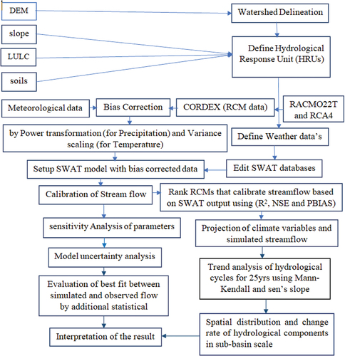
Figure 2. Flow chart for the Methodology.

(4) $\bar{Q}=0.0493A^{0.768}$(4)

(5) $\bar{Q}=0.000225A^{0.750}P{}^{0.838}$(5)

(6) $\bar{Q}=0.000378{\left(AP\right)}^{0.755}$(6)

(7) $\bar{Q}=0.0901A^{1.017}S{}^{0.606}$(7)

(8) $\bar{Q}=0.000332(AP{)}^{0.813}S{}^{0.175}$(8)

Description of regional climate models (RCMs’)

The development of the climate model has considered the global climate phenomena over the world, which may not be free of bias and models uncertainty during the simulation of climate variables (Worku et al., 2020). Several studies on the performance of regional climate models reveal that different RCM performs differently on wide ranges of the regional watershed (Heyi & Dinka, 2022). This clearly shows that the performance level of regional climate models mainly depends on their capability of covering wide areas to simulate rainfall and temperature or other related climatological variables. Most of the study that are conducted on the performance of RCM in Ethiopia considers single climatological parameters, specifically rainfall that may not realize their performance through un-directional. All climate models are not performing equally important. For example Endris et al., (2013) indicated the RCMs rainfall simulation varies along the regions, performing good in some and poorly in others. Besides emphasizing on climate impact assessment on streamflow and hydrology, this study also aimed to assess the performance of four selected climate models (RCMs) of different driving models in simulating climatic variables, as stated in Table 4. These models were used many times by scholars to model climate change impacts in Ethiopia (Dibaba, Miegel, & Demissie, 2019). Furthermore, resolutions of the models and climate change impact under extreme scenario in consideration were main reasons of selecting these models and respective scenarios. The performance of regional climate models (RCM) in this study was evaluated using time series-based indices such as correlation coefficient (r), mean average error (MAE), and root mean square error (RMSE) (Alegre et al., 2020).

Table 4. The lists of RCMs and their driving models under RCP8.5 and RCP4.5 scenarios.

GCMs	RCMs	Spatial Resolution	Historical Simulation	Future Simulation
CCCM-CanSEM2	RCA4	0.44	1980 – 2005	2006 – 2100
	CCLM4-8-17
ICHE-ECEARTH	RACMO22T
	HIRHAM5

Results

Model sensitivity, calibration, and validation

The parameterization was applied to adjust the calibration procedure with global modification terms relative to (r) and replace (v) based on soil types, land use land cover, slope, subbasin numbers and locations. Sensitive flow parameters have been effectively adjusted in the calibration process as the basins were classified into different subbasin with numerous characteristics. As a result, those parameters were prioritized during calibration using their efficiency utilizing their mean relative sensitivity value to replicate the streamflow as depicted in Table 5. Based on sensitivity analysis, Cn2.mgt, GW_DELAY.gw, Sol_AWC.sol, ESCO.bsn and SURLAG.bsn were classified as the most sensitive flow parameters, while Alfa_Bf.gw, Ch_K2.rte, Sol_K.sol, and GWqmn.gw were ranked as medium sensitive parameters within the subbasin characteristics. Table 6 shows the boundary condition of each sensitive parameters to their lower and higher limit with fitted value to the calibration.

Table 5. Flow parameters ranked according to their sensitivity from SWAT output.

Parameters name	Description	Mean relative sensitivity
r_CN2.mgt	Initial SCS runoff curve number	1.98E–01	High
r_GW_DELAY.gw	Groundwater delay	1.75E–01	High
v_Sol_AWC.sol	Available soil water capacity	9.72E–02	High
r_ESCO.bsn	Soil evaporation compensation factor	1.52E–01	High
v_SURLAG.bsn	Surface runoff lag coefficient	1.50E–01	High
v_Alfa_Bf.gw	Baseflow Alfa factor	1.46E–01	Medium
r_Ch_K2.rte	Effective hydraulic conductivity in channel	1.35E–01	Medium
v_Sol _K.sol	Soil hydraulic conductivity	1.31E–01	Medium
v_GWqmn.gw	Depth of water in the shallow aquifer	1.01E–01	Small

Table 6. Parameters used for calibration and their lowest to the highest boundary condition.

Parameters (SUFI-2)	Lower bound	Upper bound	Fitted value
CN2.mgt	−25	25	12.79
GW_DELAR.gw	1	5000	379.5
Sol_AWC. Sol	1.23	42.301	36.12
ESCO.bsn	0	5	1.18
SURLAG.bsn	0	21	14.475
Alfa_Bf.gw	0	10	7.047
Ch_K2.rte	0	10	6.025
Sol_K.sol	0	20	16.72
GWqmn.gw	0	180	142.88

The best parameters were selected depending on the model’s output during the simulation, and the simulated value was compared with observed streamflow data by giving good results while compared with other studies that have been conducted on similar subjects (He & Bao, 2021). Based on the calibration and validation results, RACMO22T simulate the streamflow very well compared to the observed and performed best with the selected performance evaluation parameters such as (PBIAS = 0.23, NSE = 0.84, R² = 0.79) for calibration and (PBIAS = 0.11, NSE = 0.88, R² = 0.81) for validation. On the other hand, the RCA4 model performs better with R² = 0.74, NSE = 0.79, PBIAS = 0.18 for calibration and R² = 0.74, NSE = 0.85 and PBIAS = 0.28 for validation as presented in (Figure 3). Therefore, the result obtained during calibration with two regional climate models indicates the model performed very well in comparison with the parameters to the standardized values after bias correction was made, as present in Table 7 and Figure 4. The computed values of time series-based indices reveal that, the model is highly capable of assessing climate change’s impact on hydrological cycles and streamflow. Indeed, when the land use land cover is unchanged, it’s a mandatory reality for the objective function to be deteriorated due to the condition of the model itself forcefully to create the difference.

Figure 3. Scatter plot of measured and simulated streamflow from RACMO22T and RCA4 models.

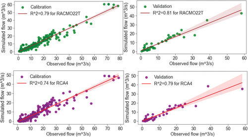
Figure 4. Calibration and validation of streamflow using two strongly performed models.

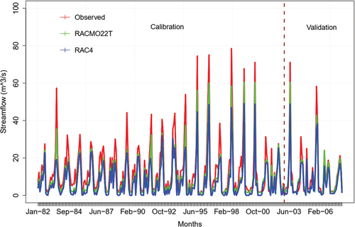
Table 7. SWAT and RCM’s performance evaluation using an objective function.

Models	Objective Function	Calibration (1982–2002)	validation (2002–2007)
RACMO22T	NSE	0.84	0.88
	R^2	0.79	0.81
	PBIAS	0.23	0.11
RCA4	NSE	0.78	0.85
	R^2	0.74	0.79
	PBIAS	0.28	0.18

When other statistical performance criteria consider basin area, mean annual rainfall and slope of the basin are used, the performance of these parameters reveals good agreement with the model output. As seen in Table 8, equations (5)(5) $\bar{Q}=0.000225A^{0.750}P{}^{0.838}$(5) , (6), (7) and (8) give good correlation agreement for observed and calibrated stream flow by RACMO22T. But for RCA4, the correlation coefficient computed by equation (4)(4) $\bar{Q}=0.0493A^{0.768}$(4) , (5) and (7) shows better agreement than other parameters. The root means square error (RMSE) calculated by equation (6)(6) $\bar{Q}=0.000378{\left(AP\right)}^{0.755}$(6) (7), and (8) shows the best agreement of observed and simulated result with both models. Hence the model’s performances by time-series metrics prove the high agreement with the output of SWAT models. However, comparing the two models for both calibration and validations, RACMO22T performed best of all according to performance criteria. On the other hand, the other statistical parameters such as skewness, kurtosis, confidences interval and mean of the simulated and observed from both regional climate models fit each other proportionally even though certain deviation was expected as shown in Table 9. But RACMO22T was still best in fit with the observed data sets.

Table 8. Times series-based performance assessment of RCMs for measured against simulated.

Stage	Models	Statistical parameters	Equations
Process	RCM	Criteria	4	5	6	7	8
Calibration	RACMO22T	r	0.81	0.785	0.792	0.8	0.79
		RMSE(m^3/s)	3.12	2.13	1.21	1.1	1.305
		MAE	1.42	1.201	1.08	1.52	1.06
Validation		r	0.852	0.793	0.821	0.81	0.813
		RMSE	1.421	1.32	1.063	1.1	0.998
		MAE	1.6	2.01	1.23	1.04	1.18
Calibration	RCA4	r	0.731	0.725	0.762	0.72	0.75
		RMSE(m^3/s)	4.22	2.16	2.151	2.2	2.205
		MAE	1.892	2.01	1.88	1.85	1.86
Validation		r	0.78	0.79	0.786	0.77	0.783
		RMSE	3.21	1.36	1.75	1.74	1.78
		MAE	1.23	1.01	1.03	1.04	1.12

Table 9. Statistical relationship of observed and simulated streamflow by frequency-based metrics.

Parameters	Observed	RACMO22T	RCA4
Mean	13.29	12.72	10.23
Skewness	2.19	2.47	2.06
Kurtosis	5.98	5.86	5.4
Confidence Intervals (95%)	1.73	1.33	1.15
Upper Limit of CI (95%)	15.03	14.05	11.38
Lower Limit of CI (95%)	11.56	11.39	9.08

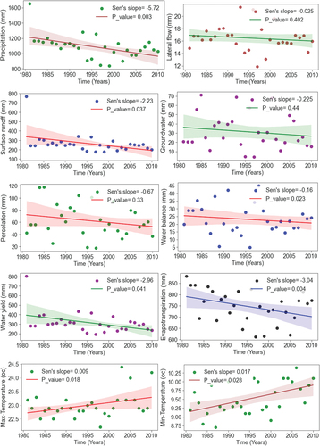
Hydro-meteorological component’s mean annual variability trend at Akaki catchment

Hydrological features are directly related to the meteorological parameters as these parameters are the core inputs for the hydrological models. According to the results obtained from the SWAT model, the annual variability trend of the simulated, the hydrological components is directly related to rainfall, evapotranspiration, maximum and minimum temperatures. The significant increasing trend of both maximum and minimum temperatures influences hydrological components to be following significant decreasing trend. In this study, the output of hydrological component for 25 years has been analyzed to identify and evaluate the climate variability in hydrology at a sub-basin level. The trend of maximum and minimum temperature was tested by Mann-Kendall test, which shows a significant increase with $p-values$of 0.018 and 0.005, respectively.

The subbasin obtains 1088.5 mm of mean rainfall on an annual basis, and the rainfall during this baseline period (1980–2005) shows a decreasing trend with $p-value$ of 0.003 in the catchments. The rise of max and min-temperature in the watershed causes the decreasing of annual rainfall by limiting hydrological cycles with a $p-value$ of 0.018 and 0.005, respectively. Such an increase in maximum and minimum temperature in the basin causing a significant decreasing trend of the hydrological components such as$WYLD$, Percolations$\left(PERC\right)$,$LA{T}_Q$,$G{W}_Q$, $PET$and $ET$ directly or indirectly, as shown in Figure 5 from the SWAT model output analysis according to Mann Kendall test which also concluded by Brhane, Raba, Beketie, Feyisa, & Siyoum, (2022), Duguma, Feyessa, & Demissie, (2021) Getahun, Li, & Pun, (2021). The average annual values of hydro-meteorological component show a decreasing pattern with 264.33 mm $\left(SURQ\right),$ 16.48 mm $\left(LA{T}_Q\right),$ 31.34 mm$\left(G{W}_Q\right)$, 62.52 mm$\left(PERC\right)$, 746.45 mm$\left(ET\right)$, 315.24 mm$\left(WYLD\right)$ and 1738.35 mm $\left(PET\right)$.

Figure 5. Mann–Kendall test (significance level 0.05) and Sen’s slope (β > 0 increasing trend and β < 0 decreasing trend) for annual variability analysis.

The correlation of major simulated hydrological components

Rainfall is the most significant climate variable that highly affects hydrological process and cycles. Because the main source of recharge for all hydrological component is the intensity of rainfall and its magnitude. The computed correlation coefficients in Table 10 show that runoff and water yields were highly correlated to precipitations with 0.89 and 0.9 respectively. This is to mean that the intensity of runoff, water yield is highly dependent on the magnitude of rainfall in the catchments.

Table 10. Correlation coefficients of major hydrological components.

Components	Rainfall	Runoff	Lateral flow	Groundwater	Percolation	Water yield
Rainfall	1	-	-	-	-	-
Runoff	0.89	1	-	-	-	-
Lateral flow	0.49	0.2	1	-	-	-
Groundwater	0.35	0.24	0.71	1	-	-
Percolation	0.35	0.19	0.66	0.95	1	-
Water yield	0.91	0.99	0.33	0.41	0.49	1

On the other hand, groundwater, percolation, and lateral flow were indirectly affected by rainfall intensity with correlation coefficients of 0.35, 0.36 and 49 respectively. Furthermore, lateral flow and percolation rate highly correlated to groundwater recharge with 0.95 and 0.71 respectively. This indicates that the magnitude of lateral flow and percolation rate is dependent on the amount of water recharged to the aquifers. In general, climate change directly affects rainfall volume and this in turn affects other dependent hydrological component and process in an integrated river basin.

Spatial variability maps of major hydrological components at subbasin level

The hydro-meteorological components resulting from SWAT model outputs are varied at subbasin level due to land use and soil variation across the catchment. These changes of parameters in each HRU through the catchment combined with climate variables that are sensitive to cause climate change are recognized in limiting hydrological cycle functions. The spatial distribution of hydrological component indicated in Figure 6 shows the spatial variability maps through interpolation on the sub-basin scale by inverse distance weighted (IDW) method, for rainfall, GW_Q, LAT_Q, PERCO, WYLD, ET, and SUR_Q using extreme scenario RCP8.5 with RACMO22T. The result indicates a considerable variation of hydrological components on subbasin level resulting from intensified climate change in the catchment.

Figure 6. The interpolated spatial variability maps of mean annual hydrological components at the subbasin scale.

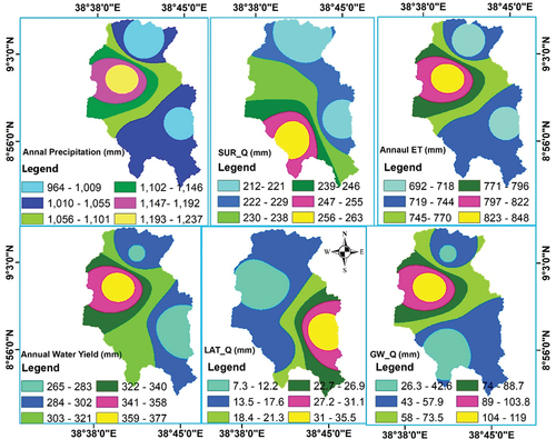
Moreover, the predicted rainfall changes indicated on the spatial map below show a significant decrease pattern in the study areas with a p-value less than 0.0001 for the baseline periods for which conclusion has been drawn by Eshete, Rigler, Shinshaw, Belete, & Bayeh, (2022). The spatial map reveals rainfall has a massive correlation and relationship with water yield, surface runoff, groundwater, percolation, and ET for this catchment. From the map, at the upper part of the basin, high annual rainfall with values of 1193 mm-1237 mm resulted in high annual water yields, groundwater, percolation, and ET. This relationship shows hydrological cycles are mainly dependent on rainfall, and their variability was caused by rainfall change due to climate change and other human-induced factors that also cause hydrological imbalance (Gedefaw & Denghua, 2023). Indeed, the spatial distributions of a hydrological components were dependent on the recharge capacity of the catchments, which is expected from the magnitude and intensity of rainfall with specified durations. Overall, the annual analysis of hydrological features in this sub-basin indicates groundwater recharge, water yield, Surface runoff, and evapotranspiration decreased by 4 %, 17.7 %, 20.8 %, 27.7 %, and 8.6 %, respectively because of climate changes.

Discussions

Rainfall trend from regional climate models for baseline periods

The increment of warm climate has been accelerating the dynamic variability of the hydrological cycle, with changes in water balance components that alter rainfall patterns and magnitude. Water stress has been profoundly affected by climate variables that govern climate change to be caused which has been concluded by Tadese et al., (2019). Climate institution of the world is developing many climate models that simulate and predict meteorological variables at different levels, considering the regional and global climate phenomena. These RCMs affect rainfall, maximum and minimum temperatures which are the most influential climate variables that highly contribute climate change to happen. Statistical analysis made on the Akaki subbasin shows that CLLM4-8-17, HIRHAM5 and RACMO22T overestimate the rainfall indices during Feburary, March, April and May (FMAM) season at Addis Ababa and sebeta stations, as seen in Figure 7.

Figure 7. Annual analysis of rainfall based on the rainfall season’s occurrences at stations.

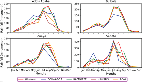
However, all the applied climate models used to simulate rainfall during the June, July, August and september (JJAS) season at Sebeta station were underestimated. But RACMO22T was closely estimated and simulate rainfall well at Addis Ababa stations. Indeed, the estimation made by RCA4 and RACMO22T during crucial rainfall season (JJAS) was better than other regional climate models, even though some deviation was still real. The computed coefficients of correlation for all models’, relative to observed climate variables was positively related except HIRHAM5. In the analysis of climate models performance to simulate rainfall and streamflow, RACMO22T and RCA4 were highly correlated. Specifically, the models was simulated the interannual variability of rainfall during summer seasons with a good correlation coefficients of 0.58 and 0.42, respectively, for RACMO22T and RCA4 (Tumsa, 2022). But in the spring season, these two RCMs were poorly performed, with correlation coefficients of 0.36 and 0.31, respectively. Rainfall is more affected by short-time seasons than long rainfall seasons during the inter-annual variability analysis.

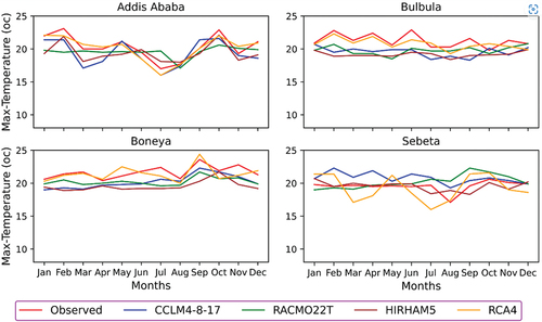
Temperature trends from regional climate models for baseline periods

SWAT model used temperature as an input to predict and simulate the situation related to hydrological processes on the earth’s surface. From the statistical analysis, temperature show an increasing trend in the catchment, which signifies the progress of global warming. The maximum and minimum temperatures were underestimated during monthly and seasonal (FMAM) and highly overestimated minimum temperatures during the summer season (JJAS) based on statistical analysis by CCLM4-8-17 and HIRHAM5 models as seen in Figure 8. But both temperatures indicate an increasing trend annually. Maximum temperature was underestimated by other models except for RCA4 during the winter season, and a similar trend was observed for its projection. Still, RCA4 and RACMO22T models experienced good performance relative to others in all seasons. These all cases which prove the versions of the two climate models mentioned above were one of the great justification for using these selected climate models to evaluate climate variability impacts on subbasin hydrology. Indeed, the trends of both maximum and minimum temperature monthly and yearly were quite different due to season inter-annual variability. CCLM4-8-17 and HIRHAM5 were completely underestimated maximum temperatures at Addis Ababa and Boneya Stations, and RACMO22T and RCA4 were overvalued at Addis Ababa station. But at Boneya station, RACMO22T underestimate and RCA4 is still overestimated. However, RACMO22T, CCLM4-8-17, and HIRHMA5 have underestimated both temperatures, but RCA4 still overestimated despite others showing an increasing trend for these temperatures on a monthly and annual basis.

Figure 8. The trends of maximum temperatures in the baseline period for each synoptic stations.

Changes in projected rainfall under the RCP4.5 and RCP8.5 scenarios

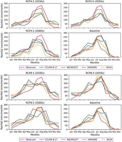
Rainfall distribution over the Akaki subbasin under both scenarios shows inconsistent trends for baseline and coming periods. According to the result obtained from RCMs for a future period in the short term (the 2030s), midterm (2050s) and long term (2080s), respectively, the rainfall value indicates increased and decreased trends for all months of the years. Rainfall is experiencing a large deviation of average rainfall season (JJAS) by −2.2, 13.5 and 7.3% under the RCP4.5 scenario in the short-term, mid-term, and long-term projection period respectively.

The average annual rainfall also increased by 5.6% during the short-term (2030s), 15.75% during the mid-term (2050s) period and decreased by 12.5% during long term (2080s) periods under RCP4.5 scenario as presented in Table 11. Moreover, under RCP8.5 scenarios, the annual rainfall decreased by 8.8% and 3.13% during the short-term (2030s) and long-term (2080s) respectively and increasing by 2.4% by mid-term (2050s). This indicates that the rainfall intensity was collectively based on the season in which mostly rainfall season occurred in (JJAS). These mean annual values of future projected rainfall under both scenarios indicate a decreasing trend.

Table 11. Percentage change in rainfall projection for both scenarios by season.

	Scenarios
	RCP4.5			RCP8.5
Seasons	2030s	2050s	2080s	2030s	2050s	2080s
JJAS	−2.2	13.5	7.3	12.1	−10.5	−25.7
FMAM	10.1	5.5	−9.2	−7.4	6.3	14.3
ONDJ	−2.3	−3.25	−10.6	−13.5	6.8	8.27

**positive sign shows increasing, and negative sign indicate decreasing.

On the other hand, from the beginning of the short term, the RCP8.5 scenario shows a high increment and decreases ultimately in the midterm and long-term periods. Average rainfall projected during JJAS, FMAM, and October, November, December, and January (ONDJ) seasons under both scenarios also offers a great variation of rainfall distribution annually and monthly from season to season. The maximum rainfall collapsed to an extreme scenario during the short-term period in JJAS and ONDJ seasons under RCP4.5, and, during the long-term period from February to May and from November to January as shown in (Figure 9). But under both scenarios and in ONDJ seasons, future projected rainfall clearly shows significant decreasing trends. The statistical analysis reveal that the projection of rainfall and temperature trend was inconsistent for the rainfall and increasing trend for temperature in the sub-basin. Moreover, the rainfall distribution in the basin is drier for the early months (December to April) for RCP4.5 and slightly shows increasing progress in rainfall season under the extreme scenario RCP8.5 which also summarized by Abdulahi, Abate, Harka, & Husen, (2022).

Figure 9. Short term, mid-term, and long-term projections of rainfall under RCP4.5 and RCP8.5 scenarios.

On the other hand, the monthly changes in rainfall were observed for the 2030s, 2050s, and 2080s periods under both scenarios. The known rainfall season from June to August shows a decreasing trend in the 2030s for RCP4.5, 2050s and 2080s for RCP8.5, as shown in (Figure 10). However, strong increasing rainfall changes were indicated under the RCP8.5 scenario during the winter and spring seasons, with decreasing trends in the summer season for the mid-term and long-terms of the analysis.

Figure 10. Monthly changes of projected rainfall based on baseline for all RCM under each scenario.

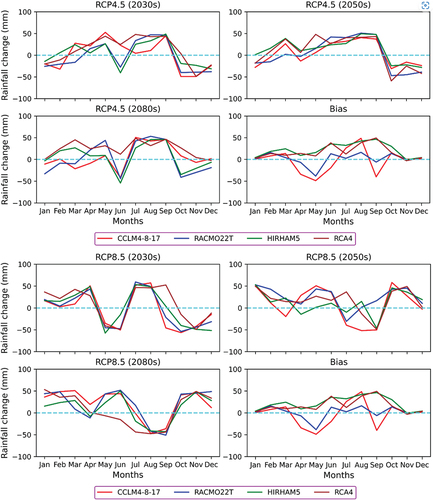
However, under the two scenarios, rainfall during the wet season (June to September) shows uniform decreasing trends. This shows that the water availability at the upper Awash subbasin in Akaki catchments for the three future horizons was governed mostly by the rainy season than the early drier periods. The general projections of water availability in this catchment, in near future, are marked by decreased trends for none rainfall season and an increase for rainfall season under both scenarios which was concluded by Taye, (2018).

Indicators of projected temperature changes under RCP4.5 and RCP8.5 scenarios

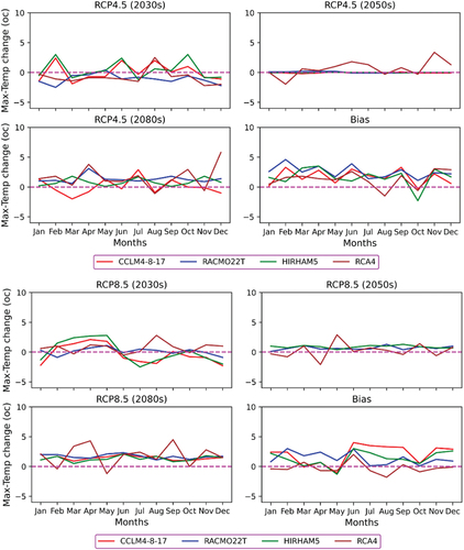
Global temperature indices have shown an ultimate increase even though the mode of rising temperatures is gradual, which leads to future global warming. According to the statistical analysis, the future projected maximum temperature for all models under both scenarios increases, as shown in Figure 11. According to the model evaluation results, CCLM4-8-17 and HIRHAM5 perform poorly, even though they show slightly increasing trends with an overlapped value under all scenarios except the 2080s for RCP4.5. The other remains a climate model that shows a rising trend under both scenarios with the best performance. For both maximum and minimum temperatures, which show an increasing trend, the models indicate a significant deviation from the observed baseline data. However, this bias has been removed using correction methods, and the changes in maximum temperature show a significant alteration from year to year in dry seasons. In the 2030s, the temperature shows a negative monthly change except for HIRHAM5 and CCLM4-8-17, and negligible changes have been observed in the 2050s under RCP4.5. In general, both maximum and minimum temperatures show an increasing change for all RCM models under RCP4.5 and RCP8.5, as shown in Figure 12.

Figure 11. Maximum temperature projections in the future under RCP4.5 and RCP8.5 scenarios.

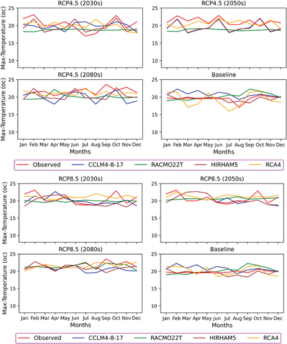
Figure 12. Monthly changes of projected maximum temperatures for all RCMs under each scenario.

Predicted climate change impacts on streamflow

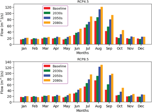
Predicted climate change on the streamflow was projected from baseline period output of the SWAT model for the first 25 years. This projected value of streamflow indicates an increasing and decreasing trend based on the rainfall and dry climate season in the catchment. The projected streamflow for the baseline period shows an increasing trend with 8.5%, 13.8% in the next thirty years (2030s), 21.3% in the midterm (2050s), and decreased at the end of long-term years (2080s) by 12.5% under RCP4.5 Scenario. Meanwhile, the trends of streamflow projected for short-, mid- and long-term periods shown a moderate increment by 2030s (12%), highly increased in 2050s by 28.5% and shows an ultimate decrease at 2080s by 9.1% under the RCP8.5 scenario, respectively, as referred on (Figure 14). In general, the projected streamflow percentage depicted below in Table 12 shows an average decrement of 1.4% and 0.3% under RCP4.5 and RCP8.5, respectively. The rise of mean average temperature and evapotranspiration throughout the catchment caused the delay of the hydrological cycle by affecting their contribution to streamflow and leading the flow to be decreased gradually. Moreover, the increase in average temperature covers a high cause for the rising of evapotranspiration and potential evaporation. These mainly caused the hydrological components in the catchment to be forced to slow the hydrological process that plays a great role to drive the rainfall in the hydrological cycle systems.

Table 12. Simulated streamflow for short, mid, and long term projected for both scenarios.

Scenarios	Baseline	2030s	2050s	2080s
RCP4.5	8.3%	13.8%	21.3%	12.5%
RCP8.5	8.3%	12.0%	28.5%	9.1%

On the other hand, the monthly projected streamflow under both scenarios shows that the flow is more varied during the main rainfall than other seasons. The changes are always positive in all scenarios from June to August, but in the winter season (December to February), the flood hydrograph shows a declining trend. In the 2030s and 2050s, the change in streamflow showed a decreasing trend in the summer for RCP4.5 and a negative trend in the Autumn seasons for RCP8.5. However, the Spring and winter seasons were the major rising events for streamflow in the 2030s and 2050s for both scenarios. But the flow shows a declining change in the long-term (2080s) period for both scenarios, as shown in Figure 13.

Figure 13. Projected streamflow changes for each season under RCP4.5 and RCP8.5 scenarios.Note: B-baseline period

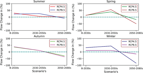
Figure 14. The projected stream flow from the reference discharge for the future scenario.

Conclusion

Streamflow in this catchment was exposed to hydro-climatological variability which imposes the extent of climate change impact in the region. The SWAT model performance was evaluated by performance criteria and gave good agreement with the result from other statistical parameters such as (NSE = 0.84, R² = 0.79, PBIAS = 0.23) for RACMO22T and (NSE = 0.78, PBIAS = 0.28, R² = 0.74,) for RCA4 during calibration. Moreover, the simulated streamflow and hydrological component from SWAT models show best fitness by the equation (5b), (5c), and (5d) and (5e), which reveals a good correlation agreement for observed and calibrated stream flow by RACMO22T. On the other hand, the correlation coefficient computed by performance equations (5a), (5b) and (5d) for RCA4 shows a strong correlation than other parameters. The relationship between recorded and simulated flow was analyzed by those time series-based indices and exhibited good agreement. The projected streamflow shows a significant decreasing pattern of 8.8% between the 2050s-2080s for RCP4.5 and 19.4% for RCP8.5 due to climate variability. However, one of the main challenges that press the water stress at upper Awash subbasins was the hydro-climatological variability deeply interrelated with inter-annual variability, mean climatological aspects and annual cycles of meteorological data. Depending on the evidence from regional climate models that capture the historical characteristics for three consecutive future periods (2030s, 2050s and 2080s), the projected streamflow under both scenarios was dependent on the basin’s climate. From this fact, it could recognize that the annual potential evapotranspiration, rainfall distribution, water yield, surface runoff, and evapotranspiration were showing a significantly decreased trend. The increasing temperature and decreasing rainfall in the basin are highly affecting the hydrological cycle, which in turn signifies an increased water deficit downstream of the catchment. The projected streamflow of Akaki river under the two scenarios shows a slightly decreasing trend despite temperatures and evapotranspiration increasing across the catchments. Furthermore, because the catchment was encircled a town where urban areas are gradually expanded, it is imperative to consider the impacts of land use land cover variability on both streamflow and hydrological process in the future. Water resource managers and policy makes should focus on this problem and need to respond quickly to reduce this climate change risks on Akaki streamflow. These all scenarios in scientific water resource management are very crucial for decision-makers to cope with global climate change.

Acknowledgments

I would like to thank the Ethiopian meteorological Agency, Ministry of Water, Irrigation, and Electricity institute for their great willingness in giving me any necessary data for the accomplishments of this research. Also, I feel many thanks to all co-authors from beginning to end for their lasting contribution and role in the achievement of this paper.

Disclosure statement

No potential conflict of interest was reported by the author(s).

Data availability statement

All necessary data used in this research paper were incorporated and included. More supplementary data will be supplied upon request.

Additional information

Funding

The research did not receive any specific fund.

References

- Abdulahi, S. D., Abate, B., Harka, A. E., & Husen, S. B. (2022). Response of climate change impact on stream fl ow: The case of the Upper Awash. Journal of Water and Climate Change, 13(2), 607–628. doi:10.2166/wcc.2021.251
- Aduah, M. S., Jewitt, G. P. W., & Toucher, M. L. W. (2017). Assessing impacts of land use changes on the hydrology of a lowland rainforest catchment in Ghana, West Africa. Water, 10(1). doi:10.3390/w10010009
- Aksoy, H., & Burgan, H. I. (2018). Annual fl ow duration curve model for ungauged basins Halil Ibrahim Burgan and Hafzullah Aksoypp. 1684–1695. doi:10.2166/nh.2018.109
- Alegre, P., Mara, P., Ferreira, D. L., Santos, P. P. D., Gonçalves, A., Fernandes, A. A., & Paiva, S. A. R. (2020). Euterpe Oleracea Mart. (Açaí) reduces oxidative stress and improves energetic metabolism in myocardial ischemia-reperfusion injury in rats. Arquivos Brasileiros de Cardiologia, 114(1), 78–86. doi:10.36660/abc.20180140
- Babar, S., & Ramesh, H. (2013). Streamflow response to land use – Land cover change over the Nethravathi River Basin. India’. doi:10.1061/(ASCE)HE.1943-5584.0001177
- Balcha, Y. A., Malcherek, A., & Alamirew, T. (2022). Understanding future climate in the upper Awash Basin. Climate, 10, 1–28.
- Bokke, A. S., Taye, M. T., Willems, P., & Siyoum, S. A. (2017). Validation of general climate models (GCMs) over upper blue nile River Basin, Ethiopia. Atmospheric and Climate Sciences, 07(1), 65–75. doi:10.4236/acs.2017.71006
- Boko, B. A., Konaté, M., Yalo, N., Berg, S. J., Erler, A. R., Bazié, P, Hwang, H. -T., Seidou, O., Niandou, A. S., Schimmel, K., & Sudicky, E. A. (2020). Watershed in Niamey, Niger. Water, 12(2), 364.
- Brhane, H., Raba, G. A., Beketie, K. T., Feyisa, G. L., & Siyoum, T. (2022). Changes in daily rainfall and temperature extremes of upper Awash Basin, Ethiopia. Scientific African, 16, e01173. doi:10.1016/j.sciaf.2022.e01173
- Chaemiso, S. E., Abebe, A., & Pingale, S. M. (2016). Assessment of the impact of climate change on surface hydrological processes using SWAT: A case study of Omo-Gibe river basin, Ethiopia’. Springer International Publishing Modeling Earth Systems and Environment, 2(4), 1–15. doi:10.1007/s40808-016-0257-9
- Daba, M.H, Kassa, T., Andualem, S., & Assefa, M. M.(2011) ‘Nile River Basin’, Nile River Basin, p. 2017. doi: 10.1007/978-94-007-0689-7.
- Daba, M. H., & You, S. (2020). Assessment of climate change impacts on river flow regimes in the upstream of awash basin, ethiopia: Based on ipcc fifth assessment report (ar5) climate change scenarios. Hydrology, 7(4), 1–22. doi:10.3390/hydrology7040098
- Dibaba, W. T., Miegel, K., & Demissie, T. A. (2019). Evaluation of the CORDEX regional climate models performance in simulating climate conditions of two catchments in Upper Blue Nile Basin. Dynamics of Atmospheres and Oceans, 87(May), 101104. doi:10.1016/j.dynatmoce.2019.101104
- Du, X., Goss, G., & Faramarzi, M. (2020). Impacts of hydrological processes on stream temperature in a cold region watershed based on the SWAT equilibrium temperature model. Water, 12(4). doi:10.3390/W12041112
- Duguma, F. A., Feyessa, F. F., & Demissie, T. A. (2021). Hydroclimate trend analysis of upper Awash Basin, Ethiopia Climate, 13,1–17.
- Emiru, N. C., Recha, J. W., Thompson, J. R., Belay, A., Aynekulu, E., Manyevere, A., Demissie, T. D., Osano, P. M., Hussein, J., Molla, M. B., Mengistu, G. M., & Solomon, D. (2022). ‘Impact of climate change on the hydrology of the upper Awash River Basin, Ethiopia (Vol. 9, pp. 3). MDPI.
- Endris, H. S., Omondi, P., Jain, S., Lennard, C., Hewitson, B., Chang'a, L., Awange, J. L., Dosio, A., Ketiem, P., Nikulin, G., Panitz, H. J., Buchner, M., Stordal, F., & Tazalika, L. (2013 November). Assessment of the performance of CORDEX regional climate models in simulating East African Rainfall Assessment of the performance of CORDEX regional climate models in simulating East African Rainfall, 26, 8453–8475. doi: 10.1175/JCLI-D-12-00708.1
- Eshete, D. G., Rigler, G., Shinshaw, B. G., Belete, A. M., & Bayeh, B. A. (2022). ‘Evaluation of streamflow response to climate change in the data ‑ scarce region, Ethiopia’. Springer International Publishing Sustainable Water Resources Management, 8(6), 1–16. doi:10.1007/s40899-022-00770-6
- Gedefaw, M., & Denghua, Y. (2023). Simulation of stream flows and climate trend detections using WEAP model in awash river basin Simulation of stream flows and climate trend detections using WEAP model in awash river basin. Cogent Engineering, 10(1). doi:10.1080/23311916.2023.2211365
- Getahun, Y. S., Li, M., & Pun, I. (2021). Jo ur na l P re of. Elsevier Ltd HELIYON, 7(9), e08024. doi:10.1016/j.heliyon.2021.e08024
- He, R., & Bao, Z. (2021). Uncertainty analysis of SWAT modeling in the lancang river basin using four different algorithms. Water, 13, 1–21.
- Heyi, E. A., & Dinka, M. O. (2022). Assessing the impact of climate change on water resources of upper Awash River sub-basin. Ethiopia’. doi:10.24425/jwld.2022.140394
- Jiqin, H., Gelata, F. T., & Chaka Gemeda, S. (2023). Application of MK trend and test of Sen’ s slope estimator to measure impact of climate change on the adoption of conservation agriculture in Ethiopia. 14(3), 977–988. doi:10.2166/wcc.2023.508
- Kang, Y., Gao, J., Shao, H., & Zhang, Y. (2020). Quantitative analysis of hydrological responses to climate variability and land-use change in the hilly-gully region of the loess plateau, China. Water, 12(1), 82. doi:10.3390/w12010082
- Khalid, K., Ali, M. F., Abd Rahman, N. F., Mispan, M. R., Haron, S. H., Othman, Z., & Bachok, M. F(2016). Sensitivity analysis in watershed model using SUFI-2 algorithm. Procedia Engineering, 162, 441–447. doi:10.1016/j.proeng.2016.11.086
- Mahmoodi, N., Wagner, P. D., Kiesel, J., & Fohrer, N. (2021). Modeling the impact of climate change on stream fl ow and major hydrological components of an Iranian Wadi system Nariman Mahmoodi (Paul D. Wagner, Jens Kiesel, & Nicola Fohrer, Ed.) pp. 1598–1613. doi:10.2166/wcc.2020.098.
- Martínez-Retureta, R., Aguayo, M., Abreu, N. J., Stehr, A., Duran-Llacer, I., Rodríguez-López, L., Sauvage, S., & Sánchez-Pérez, J. M. (2021). Estimation of the climate change impact on the hydrological balance in basins of South-Central Chile. Water, 13, 794.
- Melesse, A. M., Abtew, W., & Setegn, S. G. (2013). ‘Nile River Basin: Ecohydrological challenges, climate change and hydropolitics. Nile River Basin: Ecohydrological Challenges, Climate Change and Hydropolitics, (February), 1–718. doi:10.1007/978-3-319-02720-3
- Menna, B. Y. (2017). Simulation of Hydro climatological impacts caused by climate change: The case of hare Watershed, Southern Rift Valley of Ethiopia. Hydrology: Current Research, 08(2). doi:10.4172/2157-7587.1000276
- Negash, E. D. (2023). Effects of land use land cover change on streamflow of Akaki. In Sustainable water resources management (Vol. 4). Springer International Publishing. doi:10.1007/s40899-023-00831-4.
- Rojas-Downing, M. M., Nejadhashemi, A.P., Harrigan, T., & Woznicki, S.A. (2017). Climate change and livestock: Impacts, adaptation, and mitigation. Climate Risk Management, 16, 145–163. doi:10.1016/j.crm.2017.02.001
- Sao, D., Tasuku Keto, L. H., Tu, L. H., Thouk, P., Fitriyah, A., & Oeurng, C. (2020). Water evaluation of Di ff erent objective functions used in the SUFI-2 calibration process of SWAT-CUP on water balance analysis: A case study of the pursat. Water, 12(10), 2901. doi:10.3390/w12102901
- Tadese, M. T., Kumar, L., Koech, R.,& Zemadim, B. (2019). Hydro-climatic variability: A characterisation and trend study of the Awash River Basin Ethiopia. MDPI.
- Taye, M. T. (2018). Climate change impact on water resources in the Awash Basin, Ethiopiapp. 1–16. doi:10.3390/w10111560
- Tumsa, B. C. (2022). Performance assessment of six bias correction methods using observed and RCM data at upper Awash basin, Oromia, Ethiopia. Journal of Water and Climate Change, 13(2), 664–683. doi:10.2166/wcc.2021.181
- Worku, G., Teferi, E., Bantider, A., & Dile, Y.T. (2020). Statistical bias correction of regional climate model simulations for climate change projection in the Jemma sub-basin, upper Blue Nile Basin of Ethiopia. Theoretical and Applied Climatology, 139(3–4), 1569–1588. doi:10.1007/s00704-019-03053-x
- Yesuf, H. M., Melesse, A. M., Zeleke, G., & Alamirew, T. (2016). Streamflow prediction uncertainty analysis and verification of SWAT model in a tropical watershed. In Environmental Earth Sciences. Berlin Heidelberg: Springer. doi:10.1007/s12665-016-5636-z
- Zeberie, W. (2019). Modelling of Rainfall-Runoff Relationship in Big-Akaki Watershed, Upper Awash Basin. World News of Natural Sciences, 27(October), 108–120.
- Zhang L., Nan, Z., Xu, Y., & Li, S. (2016). Hydrological impacts of land use change and climate variability in the headwater region of the Heihe River Basin, northwest China. PLoS ONE, 11(6), 1–25. doi:10.1371/journal.pone.0158394