A novel statistical model for flood prediction in the Eel River watershed, New Brunswick, Canada

ABSTRACT

A strong correlation between the effect of climate change and the increase in flooding frequency and magnitude has been reported in Canada. Consequently, there is a crucial need to examine the effects of future climate change scenarios on flooding conditions. The main objective of this research is to better understand the destructive effects of flood events under historical and future climate change conditions for a small watershed (Eel River watershed) in New Brunswick (NB), Eastern Canada. A practical model had been developed using the modified Artificial Neural Network (ANN) in MATLAB by the authors of this study. The architecture and data structure of ANN is characterized by a back propagation with the Levenberg–Marquardt method. The observed daily total precipitation, daily maximum and minimum air temperatures, daily discharge for the period 1967 to 1983, the simulated monthly maximum and minimum air temperatures, and monthly total precipitation for the period of 1996–2099 from the CanESM2, the second-generation Canadian Earth System Model (CGCM), were used as input of the model. The Representative Concentration Pathways (RCP 4.5 and 8.5), as suitable climate change scenarios, were selected based on the Intergovernmental Panel on Climate Change (IPCC) recommendations for flood studies. Daily values of temperatures, precipitations, and discharges were converted to monthly mean values for better prediction of the output results. In addition, two series of observed discharges were prepared using mean monthly (Qavg) and daily maximum discharges (Qd) as the Target of the model. For more accurate analysis, the time frames of 1996–2012 (for the historical) and 2022–2038, 2039–2055, 2056–2072, 2073–2089, and 2083–2099 (for the future) were considered with a duration of 16 years for each time frame. The output results of ANN were predicted daily maximum (Qd) and mean (Qavg) discharges under the impact of climate change scenarios. As a part of the developed model, Flood Frequency Analysis (FFA) was undertaken using the generalized extreme value (GEV) and the three-parameter lognormal (LN3) distributions based on the predicted and observed discharges. The performance of FFA and ANN were demonstrated using the Anderson–Darling (AD), the Chi-square (CS) tests and coefficient of correlation (R) and mean squared error (MSE), respectively. In conclusion, the three most critical time frames with the highest values of predicted discharges were 2022–2038, 2056–2072, and 2073–2089 for RCP4.5 and 2039–2055, 2073–2089, and 2083–2099 for RCP8.5. Also, based on the FFA, the magnitudes of flood recurrence for the future time period of 100  years will dramatically increase according to the most critical time frames of 2056–2072 and 2039–2055 for RCP 4.5 and 8.5, respectively. Findings indicated that the Eel River watershed will encounter severe floods, and about a 50% increase in mean discharge, especially for the critical time frames. Finally, flood occurrences show increasing trends due to climate change effects in the most critical time frames.

KEYWORDS:

• ANN
• flood prediction
• climate change
• CGCM
• New Brunswick

Introduction

Floods in the context of global change can cause some major problems in relation to environmental disturbances such as urbanization, agriculture, deforestation, and so on (Alifu, Hirabayashi, Imada, & Shiogama, 2022; Arnell & Gosling, 2016; Kundzewicz et al., 2013). Flooding has always been a pervasive natural hazard in Canada due to many rivers, lakes, bodies of water, climatic conditions, and the presence of communities in floodplains (Burn & Whitfield, 2016; Public Safety of Canada, 2013). In addition, major disastrous floods that occurred in some Canadian provinces such as British Columbia, Newfoundland, and Nova Scotia in 2021 show the importance of this phenomenon. Indeed, according to the Canadian Disaster Database of the Public Safety Canada, more than 300 flood disasters have been recorded for the period 1902 to 2014, showing, on the one hand, the recurrence of the meteorological and hydrological triggering conditions and, on the other hand, the exposure and vulnerability of the population. In eastern Canada, the configuration of the river system and the climatic conditions – cold winter with significant snow cover – create favorable conditions for flooding related to snowmelt, in addition to the ice-jam formation (Gerard & Davar, 1995; Rokaya, Budhathoki, & Lindenschmidt, 2018). Disaster statistics emerged to show flood occurrences are becoming more common in the context of NB, with medium-scale events increasing fastest due to severe changes in weather patterns and climate. For example, the springs of 2017 to 2019 were especially disastrous and costly because of the seriousness of the floods (Brogan, McDonald, Lyons, Johnston, & Stewart-Robertson, 2020; Henry, Laroche, Hentati, & Boisvert, 2020; Lin, Mo, Vitart, & Stan, 2019). There are different reasons for the occurrence of floods in NB. In this province, inland flooding can occur with rapid snowmelt and heavy rainfall (Burrell et al., 2015) in addition to the water buildup behind an ice jam. In NB, due to some warm periods in wintertime, favorable to moderate ice-jam problems, flooding has dangerous effects due to the rapid melt of snow (Baronetti, Fratianni, Acquaotta, & Fortin, 2019). In other months of the year, abundant rainfall during primary storms can cause flooding, especially in smaller rivers. Moreover, coastal flooding can be triggered by storm surges or high tides (Lindenschmidt, Huokunab, Burrellc, & Beltaosd, 2018; Mallet, Fortin, & Germain, 2018). Furthermore, the land near an area of delta or brackish water can be at a certain risk of flooding due to high water levels caused by high marine tides, storm surges and river flows that can act separately or in combination (Buttle & Spence, 2016).

Climate change can induce local variability in the amount, duration, frequency, and distribution of precipitations which causes a change in flooding regimes (Gaur, Gaur, & Simonovic, 2018; Mladjic et al., 2011). In the summertime, warming of the Atlantic Ocean related to global warming impacts the Atlantic provinces such as NB by producing more hurricanes or stronger ones. Hurricanes eventually diminish in intensity as they make landfall and become post-tropical storms that bring intense rainfall and damaging winds causing major flooding to the southern part of the province of NB. Also, due to the complex system of storm-flooding, prediction and tracking of these events might become more difficult (Collins et al., 2014). Climate change could also alter the hydrologic cycle and its components (physical parameters) so this study will be helpful to improve the knowledge of how flood patterns could be affected by climate change in NB for the future time frame. Coastal flooding is expected to increase in many parts of the province (e.g. the Eel River watershed) because of rising sea levels. Environmental changes need to be integrated not only at local sea levels but also into the global sea-level rise and local land uplift or subsidence. Local sea level is predicted to rise and increase flooding, in most parts of the Atlantic, and Pacific coasts of Canada and the Beaufort coast in the Arctic, where the land is subsiding or slowly uplifting. The loss of sea ice in Atlantic Canada and the Arctic further increases the risk of damage to coastal infrastructures and ecosystems due to the larger storm surges and waves (Bush & Lemmen, 2019; McGrath, Stefanakis, & Nastev, 2015) and the absence of an ice foot on the coast. This issue must be considered for analyzing floods in NB because most of the large rivers (e.g. the Eel River) that end their course in the Atlantic Ocean or the Gulf of St. Lawrence are tidally influenced.

It is crucial to consider flooding problems including frequency and magnitude in NB with selecting an important watershed (in terms of water supply, biodiversity, agriculture, recreation, and sustainable development) such as the Eel River watershed that has the various mentioned involved parameters of flood occurrences within NB in connection to the newer version of the Canadian climate change model (4th generation) and atmospheric conditions to fill the gaps in previous studies. Previous studies mainly focused on the older version of the climate change model, the 3rd generation or the Coupled Global Climate Model (CGCM3), with a limited selection of scenarios to investigate flood issues (El-Jabi, Caissie, & Turkkan, 2016; El-Jabi, Turkkan, & Caissie, 2013). The aim of this research is to understand the effects of climate change on the Eel River watershed, one typical small watershed with all the critical parameters that are important for flood studies in the province, using the modified ANN which linked the Flood Frequency Analysis (FFA) for the historical data and the future climate projection of the 4th generation of CGCM3 which is equal to the second generation Canadian Earth System Model (CanEsm2) using two Representative Concentration Pathways scenarios (RCP 8.5 and 4.5) for the future time frame 2022–2099.

Selected study area characteristics

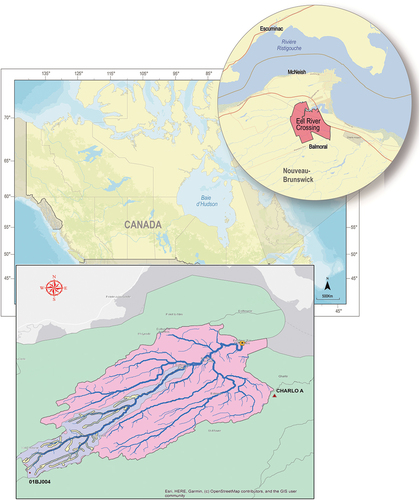
The Eel River watershed was selected as a study area due to the vulnerability of this important watershed toward various flood occurrences in NB based on Figure 1. The Eel River watershed is located in the range of Appalachian Mountain and is part of the Gulf of St. Lawrence drainage basin. The Eel River watershed is approximately 220 $\mathrm{k}{\mathrm{m}}^2$ and 24 km long. The drainage area of the Eel River station near Eel River Crossing is equal to 88.6 $\mathrm{k}{\mathrm{m}}^2$. Furthermore, the percentage of lakes and swamps in this watershed is 68%. The Eel River itself is a main watercourse in the watershed with a length of around 135 km from its headwaters to its confluence with the Restigouche River and empties into the “Chaleur” Bay. The watershed can be considered rural, with a population of about 1953 (Statistic Canada, 2017), mainly concentrated in the Eel River crossing area near the mouth of the river. The Eel River crossing village has an area of 22.79 km² and is built on a plain bordered by the Appalachians except to the east, where the “Chaleur” Bay extends. Mount Dalhousie to the north, 160 m high, is the highest point closest to the village. In addition, the Eel River crossing area is considered a Designated Watershed Protected Area (DWPR) by the Government of New Brunswick as a portion of the local population obtains their drinking water from this section of the river. Maritime Climate, with characteristics of high precipitation level and humidity, affects the Eel River watershed which brings mild summers and relatively mild winters. According to Koppen’s climate classification (Köppen & Geiger, 1930), the whole province of NB is defined as a humid continental climate (Dfb). However, according to Fortin and Dubreuil (2020), who produced a map of the different types of climates at the province scale, the study area is of East Coast type. For this climate type, the average temperature of the coldest month (January) is 0 °C, while the average temperature of the hottest month (July) is 10.1 °C, based on the reference period of 1981 to 2010. This climate type’s average annual precipitation is 1114 mm. The study area receives nearly 30% of its yearly precipitation as snow, and snow accumulation on the ground peaks at about 60.5 cm in February (Baronetti, Fratianni, Acquaotta, & Fortin, 2019). Generally, during the melt period in March and April, the risk of flooding is most significant in the province.

Figure 1. Case study area.

The geology of the Eel River watershed which is formed in the southwestern Miramichi terrane of NB includes a calc-alkaline suite of volcanic rocks that are interlayered with intervals of polylith fragmental rocks in addition to the sedimentary rocks and are overlain by a thick sedimentary sequence (McClenaghan, Lentz, & Fyffe, 2006).

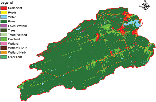
The Eel River watershed land use is divided into 89% forest, 6% cropland, and 5% urban development. Most of the territory has forests, old farmland, and wetlands and the altitude in the Eel River crossing village does not exceed 20 m. It is unlikely that this insignificant land use and land cover has a major impact on the hydrological response of the watershed (Laplante & Simard, 2013; Statistic Canada, 2023). Figure 2 shows the most recent land use map of the Eel River watershed.

Figure 2. The most recent land use map of the Eel River watershed.

Materials and methods

Data preparation

Total precipitation and daily maximum and minimum air temperatures for the recorded period 1967 to 1983 as the observed data from Charlo A station in Eel River Watershed were obtained from Environment Canada’s National Climate Data Archive, daily observed discharge (Qobs, m³/s) data from 01BJ004 hydrological station was obtained as an observed data from Environment Canada’s National Water Data Archive. Simulated monthly maximum and minimum air temperatures and total precipitation for the whole period of 1996–2099, in which 1996 to 2021 was defined as historical data and 2022 to 2099 defined as future data, were obtained from Canadian Centre for Climate Modelling and Analysis (CCCma) for simulated CanESM2/RCP4.5 and 8.5 scenarios climate change model. The main reason for choosing RCP4.5 and 8.5 is that based on the IPCC report, RCP4.5 and 8.5 are described as intermediate and high emission scenarios that are appropriate for evaluating the future effects of climate change on flood events. In RCP4.5, the emission peak will occur around 2040, then they will decline. Moreover, RCP 4.5 needs carbon dioxide (CO₂) emissions to start decreasing by 2045 to reach approximately half of the levels of 2050 by 2100. RCP4.5 is more likely than not to result in a global temperature rise between 2 °C, and 3 °C, by 2100 with a mean sea level rise 35% higher than that of RCP 2.6. Many animal and plant species will be unable to adjust to the effects of RCP4.5 and higher RCPs in the near future (Thomson et al., 2011). RCP8.5 is regarded as the highest baseline emissions among RCPs and by the year 2100, this scenario predicts a 4.5 to 6 °C temperature increase (Riahi et al., 2011).

The developed database for analysis was checked in terms of data quality to find out if there is any missing data within a time series or not. There is no missing data reported within an entire database. It is important to note that daily values of temperatures, and precipitation, are converted to monthly mean values. In addition, two series of observed discharges were prepared using mean monthly (Qavg) and daily maximum discharges (Qd) to obtain better results. The daily maximum discharge is the highest selected value of the discharge for each month. For the analysis, the time frames of 1996–2012 (for the historical) and 2022–2038, 2039–2055, 2056–2072, 2073–2089, and 2083–2099 (for the future) were considered with a duration of 16 years for each time frame. The reason for choosing 16 years interval for each time frame is to cover the whole observed discharge data for the analysis.

It is recommended to use downscaled climate change data due to the scale accuracy reasons for ANN simulations. The aim of using downscaling climate models is to fill the gap between the effects of global and local by layering local-level data over larger-scale climate models. The downscaled models are mainly related to small areas, down to 25 km², and have higher resolution than that represented by global climate model simulations (Diffenbaugh & Ashfaq, 2010). The process of downscaling was done using Delta-change approach (Camici, Brocca, Melone, & Moramarco, 2014; Hay, Wilby, & Leavesley, 2000; Keller et al., 2022). Changes in mean climate are applied as follows as a simple modification in downscaling approach:

(1) $Tn\mathrm{e}w=Tobs+Tdelta$(1)

(2) $p_{new}=p_{obs}\ast p_{Fact}$(2)

Tdelta is the difference between the climate change model’s (CGM) simulated mean temperature (projected in the future) and the historical mean temperature. Pfact is the ratio of the CGM simulated mean precipitation in the future time relative to the historical mean precipitation.

Model structure

A novel model for the prediction of Qd and Qavg under historical and climate change conditions using ANN with consideration of FFA was proposed. Figure 3 represents schematically the structure of the model which was developed and utilized in this study. There are three major stages in this model, namely: I) single station FFA; II) ANN simulation for prediction of discharges based on observed and climate change data; III) finally, FFA based on predicted Qd and Qavg which was obtained from ANN simulations.

Figure 3. Flowchart of the developed model.

In Figure 3, Tmin (new), Tmax (new), and P (new) are modified monthly minimum, and maximum temperatures, and precipitation, respectively. The simulation process was done using ANN for data prediction. The observed (Qobs) and predicted discharges (Qd and Qavg) were evaluated using the generalized extreme value (GEV) and three-parameter lognormal (LN3) as common approaches in FFA (Saf, 2009).

The foundation of the ANN used in this research is characterized by a learning algorithm that is backpropagation with the Levenberg–Marquardt method. Seventy percent (70%) of the data was used as training data, and thirty percent (30%) of the data was used as testing data. A hidden layer of 8 to 12 neurons was utilized. Figure 4 shows the structure of ANN used in this study.

Figure 4. Structure of ANN used in this research.

Probability distributions

There are numerous probability distributions (PD) used in hydrological sciences. Many different studies were carried out to understand which PD represents the best fitting for FFA. A number of PDs were proposed such as Gumbel, Normal, Lognormal, GEV, Weibull, LN3, and Gamma (Pearson type 3) in the FFA (Khosravi, Majidi, & Nohegar, 2012; Ndetei, Opere, & Mutua, 2007). For selecting an appropriate flood frequency model, several important steps should be undertaken such as an in-depth analysis of historical data, investigation of the flood magnitude using the event-descriptive variable, assessment of the acceptability among the “distribution type” and the “flood sample” to conduct a selection process. Finding the best fit probability and the calculation of its parameter were proposed as a crucial step (Bobee, Cavadias, Ashkar, Bernier, & Rasmussen, 1993; Serinaldi, Kilsby, & Lombardo, 2018). In this research, a comparison of two commonly acceptable PDs was conducted. GEV and LN3 were adopted due to their high performance and accuracy in the analysis of the statistical characteristics of the observed and predicted flood data of the Eel River watershed.

L-Moments method

The L-Moments method, previously developed based on mathematical statistics, improves the calculation process in frequency analysis studies (Stedinger & Lu, 1995). This approach, which was developed by Hosking (1990), has been widely used by hydrologists in flood-related studies. Hosking and Wallis (1997) concluded that L-moments were an alternative system of explaining the shapes of PDs. The L-moments are based on the probability-weighted moments (PWMs) of Greenwood, Landwehr, Matalas, and Wallis (1979) study. The L-Moments method has more accuracy compared to older frequency methods. Hosking (1990) indicated that the advantage of L-moment ratios in comparison to product-moment ratios (PMR) is that the former is stronger in the presence of extreme values and does not have sample size-related bounds. In addition, L-moments and L-moment ratios are more efficient than PWMs because they are more representative measures of distribution scale and shape (Hosking, 1994).

GEV and LN3 were regarded as highly accepted and accurate PDs for FFA of various regions in Canada (Faulkner, Warren, & Burn, 2016; Zhang, Stadnyk, & Burn, 2020). The reasons for choosing LN3 over other mentioned methods in NB are the feasibility of the LN3 for expressing severe flood events for gauging sites, and its accurate performance for evaluation of flood events (Aucoin, Caissie, El-Jabi, & Turkkan, 2011; Environment Canada and New Brunswick Department of Municipal Affairs and Environment, 1987). GEV with consideration of its theoretical properties is a suitable distribution for describing flood events. Moreover, according to the theory of extreme value that explains annual daily discharge maxima as a part of extreme events distribution, GEV can accurately link up a probability concerning a distribution (Coles, 2001). In addition, GEV is the best-fitted PD for the evaluation of extreme hydrological events in Canada based on Zhang, Stadnyk, and Burn (2020) research which acquired 227 Hydrometric Basin Network (RHBN) stations, the sub-set of Canadian hydrometric gauging stations, for the estimation of parameters using linear moments. Furthermore, LN3 and GEV distributions were far better choices among other approaches for flood forecasting and the best distributions for regional FFA for the selected study areas in Canada (Yue & Wang, 2004).

Generalized extreme value distribution (GEV)

Based on Robson and Reed (1999), the GEV distribution has the following cumulative density function (CDF):

(3) $F\left(x\right)=exp\left\{-\left[1-\frac{k\left(x-\mu {)}^{(}1/k\right)}{\alpha }\right]\right\}k\ne 0$(3)

(4) $F\left(x\right)=exp\left[-exp\left(-\frac{x-\mu }{\alpha }\right)\right]k=0$(4)

Where $\mu$,$\alpha$, and $k$ are the location, scale, and shape parameters, respectively. For $k>0$ ($k<0$) the variable $x$ is upper (lower) bounded to $\mu +\alpha /k$. For $k>0$ the variable $x$ is unbounded.

Three parameters lognormal (LN3)

For a random variable x, if y=ln(x-a) has a normal distribution, then x will have a lognormal distribution whose probability density function (PDF) can be developed as (Singh, 1998):

(5) $F\left(x\right)=\frac{1}{\left(x-a\right)c\sqrt{2}\pi }exp\left[\frac{-{\left[ln\left(x-a\right)-b\right]}^2}{2c^2}\right]$(5)

where a is a positive quantity defined as a lower boundary, and b and $c^2$ are the form and scale parameters of the distribution. It occurs that b and $c^2$ are respectively equal to the mean ($\bar{y}$) and variance $s_y^2$ of ln(x-a). Thus, the LN3 distribution has three parameters: a, b, and c. (x-a) represent a shifted variable. The standardized variable u is obtained in the usual order:

(6) $u=\frac{ln\left(x-a\right)-b}{c}$(6)

The CDF of the LN3 distribution can be rewritten as:

(7) $F\left(x\right)={\int }_a^x\frac{1}{\left(x-a\right)c\sqrt{2}\pi }exp[\frac{-{\left[ln\left(x-a\right)-b\right]}^2}{2c^2}\mathrm{d}x$(7)

It is not possible to describe the LN3 distribution in terms of x using the F as a function because of the integral nature of the above equation.

FFA statistical tests

Goodness-of-fit (GOF) tests

The goodness-of-fit (GOF) tests are commonly used to test whether the observed data follow a particular distribution as a calibration process. The Anderson – Darling (AD) and Chi-square (CS) tests were selected for the statistical analysis of FFA. These tests are often used in FFA and have shown good performance in the case of small sample sizes and heavy-tailed distributions (Farooq, Shafique, & Khattak, 2018; Laio, 2004; Önöz & Bayazit, 1995).

The AD test consists of the lists of critical values for GOF statistics which were calculated for various significance levels (alpha), as well as the acceptance of the null hypothesis for each of the level values. The AD statistic measures how well the data follows a particular distribution. For a specified data set and distribution, the better the distribution fits the data, the smaller this statistic will be. AD may also be considered as a “relative” measure of the GOF between different distributions (Predicted vs Observed data) for FFA.

The statistic test ($A^2)$ for AD is defined as:

$A^2$ = $-n-S$ (8)

Where S= ${\sum }_{i=1}^n\frac{\left(2i-1\right)}{n}\left[logF\left(yi\right)+log\left(1-F\left(y_{n+1-i}\right)\right)\right]$ (9)

In equation 9, n is sample size and $F\left(y_i\right)$ represents the CDF of the specified distribution.

A CS test, also written as the χ2 test, is a statistical hypothesis test that is valid to perform when the statistic test is chi-squared distributed under the null hypothesis. In general, smaller p-values are desirable according to this test. The smaller the p-value, the more certainty there is that the null hypothesis can be rejected. A very small p-value would indicate with a great deal of significance that the data distribution testing does not follow a standard normal distribution (null hypothesis).

The statistic test $\left(x^2\right)$ for CS is defined as:

(10) $x^2=\sum _{i=1}^k\frac{\left(o_i-E_i\right)}{Ei}$(10)

Where $E_i=n\left(F\left(u\right)-F\left(y_l\right)\right)$ (11)

In above equation, n is sample size and F is CDF with two variations for upper limit ($F\left(u\right)$) and lower limit $\left(F\left(y_l\right)\right)$ for the class i.

Results

The results of this study are presented in three phases: I) Single FFA without consideration of climate change effects; II) ANN simulation based on historical/future climate data; III) FFA using calculated Qd and Qavg derived from phase II.

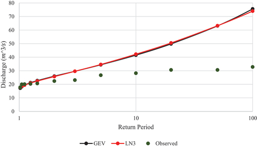
The results of the single FFA based on the comparison of GEV and LN3 distributions with observed data which is derived from the 01BJ004 hydrological station are according to Figure 5.

Figure 5. Single flood frequency analysis (FFA) using observed data (Qobs).

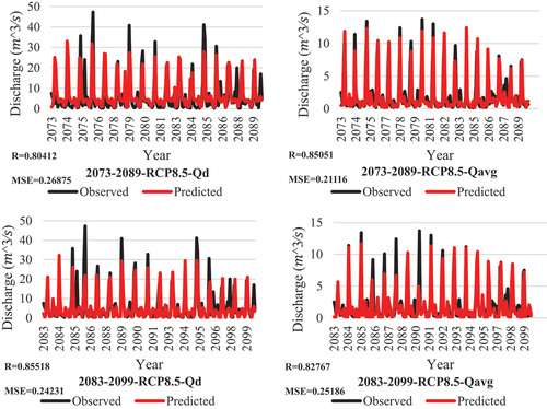
The ANN model simulated (Qd) and (Qavg) for 2022 to 2099 with selected time frames of 2022–2038, 2039–2055, 2056–2072, 2073–2089, and 2083–2099 compared to Qobs values while using modified input data (precipitation and temperatures). The three most critical time frames in terms of discharge’s magnitude were selected for RCP4.5 (2022–2038, 2056–2072, 2073–2089) and RCP8.5 (2039–2055, 2073–2089, 2088–2099). Figure 6 presents the result of the simulated Qd and Qavg compared to Qobs for mentioned time frames. This figure shows the designed ANN model has the acceptable performance and the predicted data can accurately adapt to the behavior of observed data.

Figure 6. Comparison of observed and ANN predicted (Qd and Qavg) discharges based on the RCP4.5 and RCP8.5 for the critical time frames.

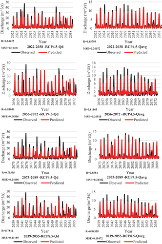
Figure 6. (Continued).

The ANN model simulated Qd and Qavg for the duration of 2022 to 2099 while using modified input data (precipitation and temperatures). Figure 7 introduces the results for the predicted Qd and Qavg for the RCP4.5 and 8.5 scenarios.

Figure 7. The total predicted discharges (Qd and Qavg) under the effects of RCP4.5 and 8.5 scenarios for the period of 2022–2099.

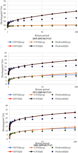
The results of FFA using GEV and LN3 for the most critical time frames based on the ANN- simulated Qd and Qavg, are illustrated in Figure 8.

Figure 8. Future FFA based on the predicted discharges (Qd and Qavg) under the effects of RCP4.5 and 8.5 scenarios for the critical time frames.

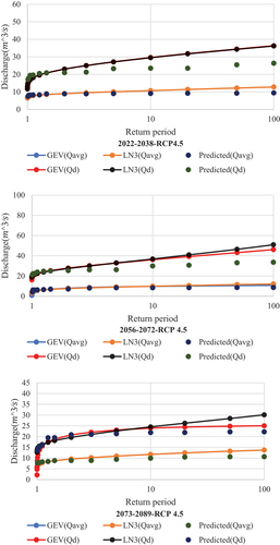
Figure 8. (Figure8b).

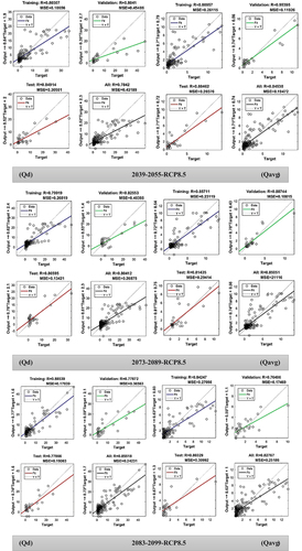
Statistical results of ANN simulations for the most critical time frames according to the coefficient of correlation (R) and mean squared error (MSE) are presented in Figure 9 for RCP4.5 and 8.5 respectively. All values of R and MSE for the “testing,” “training,” “validation,” and “total” stages were proposed. The closer the R-value to 1 the better the correlation. For MSE, the closer values to zero mean better performance of the model.

Figure 9. Statistical results of ANN simulations for the predicted discharges (Qd and Qavg) based on the RCP4.5 and RCP8.5 for the critical time frames.

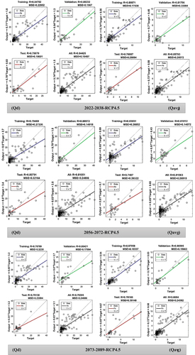
Figure 9. (Figure9b).

The statistical results of the AD for single and the future FFA are presented in Tables 1 and 2:

Table 1. AD results for GEV distribution.

Name	Statistics
Single FFA	A ^2 = 0.64467
2022–2038–4.5-Daily	A ^2 = 0.2458
2056–2072–4.5-Daily	A ^2 = 0.41285
2073–2089–4.5-Daily	A ^2 = 0.55827
2022–2038–8.5-Daily	A ^2 = 0.44686
2056–2072–8.5-Daily	A ^2 = 0.27379
2073–2089–8.5-Daily	A ^2 = 0.36612
2039–2055–4.5-Monthly	A ^2 = 0.4458
2073–2089–4.5-Monthly	A ^2 = 0.38496
2083–2099–4.5-Monthly	A ^2 = 0.37233
2039–2055–8.5-Monthly	A ^2 = 0.44686
2073–2089–8.5-Monthly	A ^2 = 0.60433
2083–2099–8.5-Monthly	A ^2 = 0.5554

Table 2. AD results for LN3 distribution.

Name	Statistics
Single FFA	A ^2 = 0.81673
2022–2038–4.5-Daily	A ^2 = 0.18814
2056–2072–4.5-Daily	A ^2 = 0.21285
2073–2089–4.5-Daily	A ^2 = 0.35827
2022–2038–8.5-Daily	A ^2 = 0.4047
2056–2072–8.5-Daily	A ^2 = 0.26445
2073–2089–8.5-Daily	A ^2 = 0.28819
2039–2055–4.5-Monthly	A ^2 = 0.2458
2073–2089–4.5-Monthly	A ^2 = 0.37249
2083–2099–4.5-Monthly	A ^2 = 0.36041
2039–2055–8.5-Monthly	A ^2 = 0.42063
2073–2089–8.5-Monthly	A ^2 = 0.30433
2083–2099–8.5-Monthly	A ^2 = 0.1554

The statistical results of the CS for single and the future FFA are presented in Tables 3 and 4:

Table 3. CS results for GEV distribution.

Name	Statistics	P-value
Single FFA	X ^2 =  = 5.75	0.0464
2022–2038–4.5-Daily	X ^2 = 3.12	0.0543
2056–2072–4.5-Daily	X ^2 = 2.41	0.0594
2073–2089–4.5-Daily	X ^2 = 8.06	0.0178
2022–2038–8.5-Daily	X ^2 = 1.71	0.0562
2056–2072–8.5-Daily	X ^2 = 3.54	0.0504
2073–2089–8.5-Daily	X ^2 = 2.89	0.0594
2039–2055–4.5-Monthly	X ^2 = 2.41	0.0573
2073–2089–4.5-Monthly	X ^2 = 4.53	0.0512
2083–2099–4.5-Monthly	X ^2 = 3.82	0.0578
2039–2055–8.5-Monthly	X ^2 = 5.96	0.0565
2073–2089–8.5-Monthly	X ^2 = 5.65	0.0530
2083–2099–8.5-Monthly	X ^2 = 1.71	0.0562

Table 4. CS results for LN3 distribution.

Name	Statistics	P-value
Single FFA	X ^2 = 2.75	0.0528
2022–2038–4.5-Daily	X ^2 = 4.12	0.0504
2056–2072–4.5-Daily	X ^2 = 3.45	0.0394
2073–2089–4.5-Daily	X ^2 = 14.41	0.0007
2022–2038–8.5-Daily	X ^2 = 3.82	0.0578
2056–2072–8.5-Daily	X ^2 = 4.71	0.0562
2073–2089–8.5-Daily	X ^2 = 5.82	0.0578
2039–2055–4.5-Monthly	X ^2 = 3.71	0.0562
2073–2089–4.5-Monthly	X ^2 = 5.53	0.0539
2083–2099–4.5-Monthly	X ^2 = 4.41	0.0594
2039–2055–8.5-Monthly	X ^2 = 6.64	0.0530
2073–2089–8.5-Monthly	X ^2 = 6.24	0.0330
2083–2099–8.5-Monthly	X ^2 = 3.82	0.0278

Discussion

The results of the study were obtained in three definitive phases. First, the results of a single FFA for the 01BJ004 hydrological station in the Eel River watershed using GEV and LN3 approaches were obtained. The aim of utilizing a single FFA is to predict the discharge for the future time (100 years) without consideration of climate change effects. Based on Figure 5, and Tables 1 to 4, it is observed that GEV is a better fitting method for the prediction of discharge due to the smaller values of A ² and P-value based on the AD and CS tests, respectively.

For the prediction of Qd and Qavg using ANN with modified input data under the influence of RCP4.5 and 8.5 scenarios, the future period 2022–2099 was considered. For obtaining better results, the future period was divided into five intervals of 2022–2038, 2039–2055, 2056–2072, 2073–2089, and 2083–2099. The reason for choosing 16  years of duration for each interval is the better adaptability and comparison with available Qobs. Based on the obtained results from the simulation process, the three most critical time frames with the highest values of predicted discharges were selected for RCP4.5 (2022–2038, 2056–2072, 2073–2089) and RCP8.5 (2039–2055, 2073–2089, 2083–2099). It is concluded that the developed novel model can accurately predict Qd and Qavg for RCP4.5 and 8.5 based on the comparison of predicted versus observed data and the acceptable statistical results in Figure 6. It is worth mentioning that ANN results based on Figure 6 miss the highest peaks in some years and there is a shift in time in some instances due to the preprogrammed selection of training data by the model, the complexity in the architecture design of ANN, and the importance of hyperparameters in the design phase of ANN, such as learning rate and regularization strength. Moreover, according to Figure 9, it is observed that R and MSE have acceptable values, the more the R and MSE values are respectively closer to 1 and 0 the better the performance of the model, for the (“training,” “validation,” “test,” and “total”) sections. This derived fact shows that the developed model is working very well for the prediction of future Qd and Qavg by means of the accurate correlation between predicted and observed data.

The predicted Qd and Qavg with consideration of the RCP4.5 and 8.5 scenarios using ANN for the entire future period including the most critical time frames represented in Figure 7. The model simulation results show the higher values of Qd in comparison to Qavg for the two scenarios. The main reason for the differences between the two series of predicted discharges is a selection of observed discharge data for the Target section of the ANN model. The observed Qd has higher values in comparison to the observed Qavg. The predicted Qd has the highest values between 2054 and 2068 for RCP4.5, while the highest values for RCP8.5 were predicted between 2041 and 2051. For the predicted Qavg, the highest values occurred between 2023 to 2035 and 2078 to 2099 for RCP4.5, while RCP8.5 has the highest values between 2039 to 2055 and 2065 to 2084.

FFA based on the predicted Qd and Qavg, which was obtained by ANN simulation, was done using the GEV and LN3 approaches according to Figure 8. This figure compared the output data of FFA based on the predicted Qd and Qavg in two series (RCP 4.5 and 8.5) for the most critical time frames. According to this figure, the highest projected discharges were recorded in two critical time frames of 2056–2072 and 2039–2055 for RCP 4.5 and 8.5, respectively. Furthermore, the FFA based on the Qd has higher values of projected discharges in comparison to the FFA according to the Qavg due to the higher values of the predicted Qd for each critical time frame. Moreover, for critical time frames of 2056–2072 and 2073–2089 based on the Qd of RCP4.5, LN3 has a better performance in comparison to GEV. On the other hand, for the critical time frames of 2073–2089 and 2083–2099, according to the Qavg of RCP8.5, LN3 has better performance compared to GEV.

LN3 is a better fitting approach for the future FFA related to the critical time frames of 2056–2072 and 2073–2089 for the predicted Qd of RCP4.5 and 2073–2089 and 2083–2099 for the predicted Qavg of RCP8.5 based on the statistical results from Tables 1 to 4 which were derived according to the CS and AD tests. For the mentioned time frames, P-values LN3 are less than GEV according to Tables 1 and 2 of the CS test, and statistics (A ²) LN3 are less than GEV based on Tables 3 and 4 of the AD test, so it shows that LN3 is a better fitting approach than GEV. For other time frames, the statistical results were in acceptable ranges of fitting (P-values ≤0.05 of the CS test and equal statistics of the AD test), and no significant differences were observed between the performance of GEV and LN3.

Conclusion

Climate change will undoubtedly alter flood problems in the Eel River watershed according to the obtained results from Figures 5–8. The success of industries (e.g. agriculture, forestry, recreational fisheries, and others) intrinsically linked to the climate conditions, are making NB watersheds such as the Eel River watershed particularly vulnerable to flooding occurrences. Other factors, such as changes in land cover and land use, are also likely to modify flows in the watershed. Shuster, Bonta, Thurston, Warnemuende, and Smith (2005) mentioned that the land used development strongly correlates with the population growth proportion. This tends to increase the ratio of the impervious catchment surfaces, translating into faster surface runoff and, therefore, faster and more intense peak flooding. Such conditions would then be conducive to flooding. However, recent data for the region indicate a decrease (−5.6% by Statistic Canada, 2023) in population between 2016 and 2021, and very few developments occur during the same period in the Eel River watershed. Although development remains a possibility, nothing currently suggests this scenario. Recently, de Souza Cruz (2021) carried out a study to simulate flooding by considering changes in future climate (RCP 4.5 and RCP8.5) in combination with changes in land use in a Riverview neighborhood located southeast of the NB. Based on this research, it is concluded that the most significant change (76% increase in flood discharge) would occur in the case of intensive development (clearcutting of an urban woodlot) and the RCP8.5 scenario over a 2100 horizon. It should be noted that, according to the results of this study, climate change plays a less significant role. In contrast, land surface modification plays a much more critical role in modifying the hydrological regime and as an explanatory source of simulated future flooding. In the case of the Eel River watershed, the expected changes will be mainly caused by climate, as little development is expected in this devitalized region (Laplante & Simard, 2013).

The ANN model was effective in predicting the different flow components (Figures 6 and 7) using historical and future climate data. In addition, according to the statistical analysis (Figure 9), all the simulation steps were done accurately, and the output results had acceptable precision (Figure 6). According to the obtained results from the ANN simulation process, the three most critical time frames with the highest values of predicted discharges were 2022–2038, 2056–2072, and 2073–2089 for RCP4.5 and 2039–2055, 2073–2089, and 2083–2099 for RCP8.5. Moreover, it is concluded that based on the FFA the magnitudes of flood recurrence for the future time period of 100 years will dramatically increase based on the most critical time frames. The most significant increase will occur in 2056–2072 and 2039–2055 for RCP 4.5 and 8.5, respectively (Figure 8), which means floods with bigger discharge magnitudes will hit the Eel River watershed due to the climate change effects.

The reliability of the results is so crucial for decision-makers and government sectors. In this regard, these results (predicted discharge from ANN and projected discharges from the single and FFA) appear very significant for decision-makers and government in order to cope with the potentially disastrous effects of climate change on flood magnitudes, especially during the critical time frames in the Eel River watershed. The analyses showed that the Eel River watershed will be impacted by severe floods by comparison of projected verse predicted discharges with about a 50% increase in Qd and Qavg for each critical time frame based on Figure 8. The upward trend of increase in discharges is one of the indications of climate change effects on future flood occurrence in this watershed.

Understanding the nature and potential consequences of climate change at a regional scale in an ungauged context remains a challenge. So, future studies are needed to take into consideration the ungauged contexts under climate change issues to produce regional equations that suit the NB context. In addition, land use and land cover changes might also affect flooding, but it is difficult at this time to extrapolate future development or any exogenous disturbances in this watershed. Moreover, the main limitation of using ANN is the fixed number of input layers within an architecture of the model that causes taking fixed input and output for any operation. So, for many pattern recognition tasks, this is a limiting constraint. In order to improve the performance of the ANN model in terms of the detection of the highest peaks for all years and satisfy the issue of shifting in time, firstly it is recommended to increase the diversity selection of the samples in the training dataset, especially those that represent extreme events and variations in the highest peaks, to give the ANN a better basis for learning and generalization. Secondly, to capture the complexity of the forecast more accurately, the model architecture can be modified. This can involve investigating various network topologies, deepening the network, or adding extra layers or nodes to help the model learn more complex patterns. Thirdly, by modifying parameters like learning rate, regularization strength, or batch size within a model architecture, the ability of the ANN model to effectively capture the highest peaks can be increased.

Disclosure statement

No potential conflict of interest was reported by the author(s).

Data availability statement

The database used in this study is available upon reasonable request by the corresponding author.

References

- Alifu, H., Hirabayashi, Y., Imada, Y., & Shiogama, H. (2022). Enhancement of river flooding due to global warming. Scientific Reports, 12(1), 20687. doi:10.1038/s41598-022-25182-6
- Arnell, N. W., & Gosling, S. N. (2016). The impacts of climate change on river flood risk at the global scale. Climatic Change, 134(3), 387–401. doi:10.1007/s10584-014-1084-5
- Aucoin, F., Caissie, D., El-Jabi, N., & Turkkan, N. (2011). Flood frequency analyses for New Brunswick rivers. Canadian Technical Report of Fisheries and Aquatic Sciences, 2920, xi + 77.
- Baronetti, A., Fratianni, S., Acquaotta, F., & Fortin, G. (2019). A quality control approach to better characterize the spatial distribution of snow depth over New Brunswick, Canada. International Journal of Climatology, 39(14), 5470–5485. doi:10.1002/joc.6166
- Bobee, B., Cavadias, G., Ashkar, F., Bernier, J., & Rasmussen, P. (1993). Towards a systematic approach to comparing distributions used in flood frequency analysis. Journal of Hydrology, 142(1–4), 121–136. doi:10.1016/0022-1694(93)90008-W
- Brogan, B., McDonald, J., Lyons, B., Johnston, P., & Stewart-Robertson, G., 2020. Climate change adaptation plan for Saint John. Published by Atlantic coastal action program [ASAP] Saint John.
- Burn, D. H., & Whitfield, P. H. (2016). Changes in floods and flood regimes in Canada. Canadian Water Resources Journal / Revue Canadienne des Ressources Hydriques, 41(1–2), 139–150. doi:10.1080/07011784.2015.1026844
- Burrell, B. C., Huokuna, M., Beltaos, S., Kovachis, N., Turcotte, B., & Jasek, M., 2015. Flood hazard and risk delineation of ice-related floods: Present status and outlook, CGU HS Committee on River Ice Processes and the Environment, 18th Workshop on the Hydraulics of Ice-Covered Rivers Quebec City, QC, Canada.
- Bush, E., & Lemmen, D. S. (Eds.). (2019). Canada’s Changing Climate Report (p. 444). Ottawa,On: Government of Canada.
- Buttle, J. M., & Spence, C. (2016). Editors’ Note. Canadian Water Resources Journal / Revue Canadienne des Ressources Hydriques, 41(1–2), 1–1. doi:10.1080/07011784.2016.1164495
- Camici, S., Brocca, L., Melone, F., & Moramarco, T. (2014). Impact of climate change on flood frequency using different climate models and downscaling approaches. Journal of Hydrologic Engineering, 19(8), 04014002. doi:10.1061/(ASCE)HE.1943-5584.0000959
- Coles, S. (2001). An introduction to statistical modeling of extreme value (p. 224). Springer. doi:10.1007/978-1-4471-3675-0
- Collins, M. J., Kirk, J. P., Pettit, J., DeGaetano, A. T., McCown, M. S. … Zhang, X. (2014). Annual floods in New England (USA) and Atlantic Canada: Synoptic climatology and generating mechanisms. Physical Geography, 35(3), 195–219. doi:10.1080/02723646.2014.888510
- de Souza Cruz, A. M. 2021. Les Impacts des Changements Climatiques sur le réseau de Drainage: Le Cas de la Portion urbanisée du Bassin Versant de Mill Creek, Nouveau-Brunswick. Universite de Moncton (Canada). Master Thesis.
- Diffenbaugh, N. S., & Ashfaq, M. (2010). Intensification of hot extremes in the United States. Geophysical Research Letters, 37(15), L1570. doi:10.1029/2010GL043888
- El-Jabi, N., Caissie, D., & Turkkan, N. (2016). Flood analysis and flood projections under climate change in New Brunswick. Canadian Water Resources Journal / Revue Canadienne des Ressources Hydriques, 41(1–2), 319–330. doi:10.1080/07011784.2015.1071205
- El-Jabi, N., Turkkan, N., & Caissie, D. (2013). Regional climate index for floods and droughts using Canadian Climate Model (CGCM3.1). American Journal of Climate Change, 2(2), 106–115. doi:10.4236/ajcc.2013.22011
- Environment Canada and New Brunswick Department of Municipal Affairs and Environment. (1987). Flood frequency analyses, New Brunswick, a guide to the estimation of flood flows for New Brunswick rivers and streams (p. 49). Department of Municipal Affairs and Environment, New Brunswick: Water Resources Planning Branch.
- Farooq, M., Shafique, M., & Khattak, M. S. (2018). Flood frequency analysis of river swat using log Pearson type 3, generalized extreme value, normal, and Gumbel max distribution methods. Arabian Journal of Geosciences, 11(9), 216. doi:10.1007/s12517-018-3553-z
- Faulkner, D., Warren, S., & Burn, D. (2016). Design floods for all of Canada, Canadian Water Resources Journal / Revue Canadienne des Ressources Hydriques, 41(3), 398–411. doi:10.1080/07011784.2016.1141665
- Fortin, G., & Dubreuil, V. A. (2020). A geostatistical approach to create a new climate types map at regional scale: Case study of New Brunswick, Canada. Theoretical and Applied Climatology, 139(1–2), 323–334. doi:10.1007/s00704-019-02961-2
- Gaur, A., Gaur, A., & Simonovic, S. P. (2018). Future changes in flood hazards across Canada under a changing climate. Water, 10(10), 1441. doi:10.3390/w10101441
- Gerard, R., & Davar, K. S. (1995). Chapter 1: Introduction. In S. Beltaos (Ed.), River Ice Jams (pp. 1–28). Highlands Ranch: Water Resources Publications.
- Greenwood, J. A., Landwehr, J. M., Matalas, N. C., & Wallis, J. R. (1979). Probability weighted moments: Definition and relation to parameters of several distributions expressable in inverse form. Water Resources Research, 15(5), 1049–1054. doi:10.1029/WR015i005p01049
- Hay, L. E., Wilby, R. L., & Leavesley, G. H. (2000). A comparison of delta change and downscaled GCM scenarios for three mountainous Basins in the United States. JAWRA Journal of the American Water Resources Association, 36(2), 387–397. doi:10.1111/j.1752-1688.2000.tb04276.x
- Henry, S., Laroche, A. M., Hentati, A., & Boisvert, J. (2020). Prioritizing Flood-Prone Areas Using Spatial Data in the Province of New Brunswick, Canada. Geosciences, 10(12), 478. doi:10.3390/geosciences10120478
- Hosking, J. R. M. (1990). L-moments: Analysis and estimation of distributions using linear combinations of order statistics. Journal of the Royal Statistical Society: Series B (Methodological), 52(1), 105–124. doi:10.1111/j.2517-6161.1990.tb01775.x
- Hosking, J. R. M. (1994). The four-parameter kappa distribution. IBM Journal of Research and Development, 38(3), 251–258. doi:10.1147/rd.383.0251
- Hosking, J. R. M., & Wallis, J. R. (1997). Regional. frequency analysis: An approach based on L-moments. Cambridge University Press. doi:10.1017/CBO9780511529443
- Keller, A. A., Garner, K. L., Rao, N., Knipping, E., Thomas, J., & Muhammad, S. (2022). Downscaling approaches of climate change projections for watershed modeling: Review of theoretical and practical considerations. PLOS Water, 1(9), e0000046. doi:10.1371/journal.pwat.0000046
- Khosravi, G., Majidi, A., & Nohegar, A. (2012). Determination of suitable probability distribution for annual mean and peak discharges estimation (case study: Minab river-barantin gage, Iran). International Journal of Probability and Statistics, 1(5), 160–163. doi:10.5923/j.ijps.20120105.03
- Köppen, W., & Geiger, R. (1930). Handbuch der klimatologie (Vol. 1). Berlin: Gebrüder Borntraeger.
- Kundzewicz, Z. W., Kanae, S., Seneviratne, S. I., Handmer, J., Nicholls, N. … Sherstyukov, B. (2013). Flood risk and climate change: Global and regional perspectives. Hydrological Sciences Journal, 59(1), 1–28. doi:10.1080/02626667.2013.857411
- Laio, F. (2004). Cramer–von Mises and Anderson–Darling goodness of fit tests for extreme value distributions with unknown parameters. Water Resources Research, 40(9), W09308. doi:10.1029/2004WR003204
- Laplante, P., & Simard, M. (2013). Les enjeux et les défis du développement territorial durable dans une région à problèmes: le cas du comté de Restigouche au Nouveau-Brunswick. Revue de l’Université de Moncton, 44(1), 111–143. doi:10.7202/1029305ar
- Lindenschmidt, K. E., Huokunab, M., Burrellc, B. C., & Beltaosd, S. (2018). Lessons learned from past ice-jam floods concerning the challenges of flood mapping. International Journal of River Basin Management, 16(4), 457–468. doi:10.1080/15715124.2018.1439496
- Lin, H., Mo, R., Vitart, F., & Stan, C. (2019). Eastern Canada flooding 2017 and its subseasonal predictions. Atmosphere-Ocean, 57(3), 195–207. doi:10.1080/07055900.2018.1547679
- Mallet, J., Fortin, G., & Germain, D. (2018). Extreme weather events in northeastern New Brunswick (Canada) for the period 1950–2012: Comparison of newspaper archive and weather station data. The Canadian Geographer Geographe Canadien, 62(2), 130–143. doi:10.1111/cag.12411
- McClenaghan, S. H., Lentz, D. R., & Fyffe, L. R. (2006). Chemostratigraphy of volcanic rocks hosting massive sulfide clasts within the meductic group, west-central new Brunswick. Exploration and Mining Geology, 15(3–4), 241–261. doi:10.2113/gsemg.15.3-4.241
- McGrath, H., Stefanakis, E., & Nastev, M. (2015). Sensitivity analysis of flood damage estimates: A case study in Fredericton, New Brunswick. International Journal of Disaster Risk Reduction, 14(4), 379–387. doi:10.1016/j.ijdrr.2015.09.003
- Mladjic, B., Sushama, L., Khaliq, M. N., Laprise, R., Caya, D., & Roy, R. (2011). Canadian RCM projected changes to extreme precipitation characteristics over Canada. Journal of Climate, 24, 2565–2584. doi:10.1175/2010JCLI3937.1
- Ndetei, C., Opere, A., & Mutua, F. (2007). Flood frequency analysis in lake Victoria basin based on tail behaviour of distributions. Kenya Meteorological Society (KMS), 1, 44–54.
- Önöz, B., & Bayazit, M. (1995). Best-fit distributions of largest available flood samples. Journal of Hydrology, 167(1–4), 195–208. doi:10.1016/0022-1694(94)02633-M
- Public Safety of Canada, 2013. https://www.publicsafety.gc.ca/cnt/mrgnc-mngmnt/ntrl-hzrds/fld-en.aspx
- Riahi, K., Rao, S., Krey, V., Cho, C., Chirkov, V. … Rafaj, P. (2011). RCP 8.5—A scenario of comparatively high greenhouse gas emissions. Climatic Change, 109(1–2), 33. doi:10.1007/s10584-011-0149-y
- Robson, A., & Reed, D. (Eds.) (1999). Statistical procedures for flood frequency estimation. In Flood estimation handbook (Vol. 3, pp. 338). Wallingford: Centre for Ecology and Hydrology.
- Rokaya, P., Budhathoki, S., & Lindenschmidt, K. E. (2018). Trends in the timing and magnitude of ice-jam floods in Canada. Scientific Reports, 8(1), 5834. doi:10.1038/s41598-018-24057-z
- Saf, B. (2009). Regional flood frequency analysis using L-moments for the West Mediterranean region of Turkey. Water Resources Management, 23(3), 531–551. doi:10.1007/s11269-008-9287-z
- Serinaldi, F., Kilsby, C. G., & Lombardo, F. (2018). Untenable nonstationarity: An assessment of the fitness for purpose of trend tests in hydrology. Advances in Water Resources, 111, 132–155. doi:10.1016/j.advwatres.2017.10.015
- Shuster, W. D., Bonta, J., Thurston, H., Warnemuende, E., & Smith, D. R. (2005). Impacts of impervious surface on watershed hydrology: A review. Urban Water Journal, 2(4), 263–275. doi:10.1080/15730620500386529
- Singh, V. P. (1998). Three-parameter lognormal distribution, entropy-based parameter estimation in hydrology. Water Science and Technology Library. Springer, 30. doi:10.1007/978-94-017-1431-0_7
- Statistic Canada, 2017. New Brunswick [Province] and Canada [Country] (table). Census Profile. 2016 Census. Statistics Canada Catalogue no. 98-316-X2016001.
- Statistic Canada, 2023. Profile table, Census Profile, 2021 Census of Population - Eel River Crossing, Village (VL) [ Census subdivision], New Brunswick (statcan.gc.ca)
- Stedinger, J. R., & Lu, L. H. (1995). Appraisal of regional and index flood quantile estimators. Stochastic Hydrology and Hydraulics, 9(1), 49–75. doi:10.1007/BF01581758
- Thomson, A. M., Calvin, K. V., Smith, S. J., Page Kyle, G., Volke, A. … Edmonds, J. A. (2011). RCP4.5: A pathway for stabilization of radiative forcing by 2100. Climatic Change, 109(1–2), 77. doi:10.1007/s10584-011-0151-4
- Yue, S., & Wang, C. Y. (2004). Possible regional probability distribution type of Canadian annual streamflow by L-moments. Water Resources Management, 18(5), 425–438. doi:10.1023/B:WARM.0000049145.37577.87
- Zhang, Z., Stadnyk, T. A., & Burn, D. H. (2020). Identification of a preferred statistical distribution for at-site flood frequency analysis in Canada. Canadian Water Resources Journal / Revue Canadienne des Ressources Hydriques, 45(1), 43–58. doi:10.1080/07011784.2019.1691942