Accurate prediction of salinity in Chott Djerid shallow aquifers, southern Tunisia: Machine learning model development

ABSTRACT

A backpropagation neural network (BPNN) was used to predict salinity levels in the Chott Djerid shallow aquifers. A set of 51 water samples was collected from the Chott Djerid plio-quaternary aquifers for geochemical analysis. Major elements and nitrates were ascertained by using high performance liquid-ion chromatography. The BPNN was trained on a dataset of 51 water samples with variable geochemical parameters. Our results indicated a high accuracy when applying a model with 13 inputs, 1 hidden layer (6 neurons) and 1 output (TDS in mg/L). The collected data were split into 80% for training the model and 20% for testing and cross validation. The result was evaluated using various statistical performance criteria (i.e., MSE, RMSE, R2, SSE, SD, Accuracy, Sensitivity, specificity, and Kappa test); it showed that BPNN model properly predicted the salinity of the Chott Djerid plio-quaterny water samples (RMSE = 0.0402; R2 = 0.9721 and SSE = 0.0146). The BPNN was able to capture the complex relationship between salinity levels and other aquifer parameters. The potential application of BPNNs for predicting salinity levels in shallow aquifers was crucial in supporting decision-makers for water management; it provided valuable insights into the salinity fluctuation of the studied shallow aquifers.

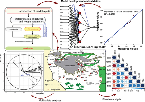
GRAPHICAL ABSTRACT

KEYWORDS:

• Artificial neural network
• salinity prediction
• groundwater management
• Chott Djerid shallow aquifers
• geochemical assessment

Introduction

Groundwater is a vital resource that has to be managed carefully. By understanding the benefits and challenges of groundwater, one can ensure its availability for future generations in a context of sustainable development (Dhaouadi, Besser, Karbout, Wassar, & Alomrane, 2021). Form this point of view, the Chott Djerid shallow aquifer system is a vital water resource for the people of Southwestern Tunisia. It includes numerous small aquifers, but important for local agriculture and drinking water supply. Hereafter, the term “Chott Djerid shallow aquifer” is intended to describe the whole sub-aquifers of the plio-quaternary system. The main aquifer is located in the Chott Djerid basin, which is a large depression in the Sahara desert (Dassi, 2011; Kraiem, Zouari, Chkir, & Agoune, 2014; Stivaletta, Barbieri, Picard, & Bosco, 2009).

The Nefzaoua aquifer is also a complex aquifer system located in the southern Tunisia with a multilayer aquifer, of which the Plio-Quaternary (PQ) is the youngest shallow aquifer lodged in sand and gravel porous layer. The Chott Djerid shallow aquifer is recharged by rainfall and runoff from the surrounding mountains. The aquifer is also recharged by the inflow of water from the Continental Intercalaire aquifer, which is a deeper aquifer located beneath the Chott Djerid basin. It is being used for a variety of purposes, including drinking water, irrigation, and industrial water supply. The Chott Djerid shallow aquifers are nonrenewable resources being depleted by overexploitation, in addition to the pollution by agricultural runoff and industrial effluents. Therefore, they face several challenges (e.g., overexploitation, pollution by agricultural runoff and industrial effluents and climate change). Those serious challenges are complicating an easy and sustainable management of the Chott Djerid shallow aquifers. Therefore, it is important to manage this valuable resource sustainably and to protect it from the threats it faces by taking immediate action for future generations (Jamei et al., 2022). The basin is home to a number of salt lakes, including Chott Djerid, as the largest lake in Tunisia, which provokes groundwater salinity (Stivaletta et al., 2009; Yebdri, Hadji, Harek, & Marok, 2021). Salinity can make groundwater unfit for drinking, irrigation, and industrial use because of several natural and anthropic factors (e.g., evaporation, irrigation, and industrial wastewater disposal). Thus, the assessment of groundwater salinity is needed for an efficient and sustainable water resource management. A number of methods were used to assess water salinity; most of them are based on the collection of water samples and measurement of the concentration of dissolved salts (Rani & Sasidhar, 2011; Sabzevar, Rezaei, & Khaleghi, 2021; Sahu, Gogoi, & Nayak, 2021). However, those methods can be time-consuming and expensive.

A more efficient and cost-effective way to assess groundwater salinity is artificial neural networks (ANNs). They are powerful for water salinity prediction; they have been shown to be more accurate than traditional statistical methods, and they can be used to predict salinity in a variety of water bodies. Khudhair, Zubaidi, Al-Bugharbee, Al-Ansari, and Ridha (2022) used ANN to predict monthly salinity data for the Euphrates river in Iraq. The ANN model was trained on historical data from 2010 to 2019, and it was able to accurately predict salinity levels up to one year in advance. Similarly, Al-Waeli, Sahib, and Abbas (2022) successfully predicted salinity in groundwater in the West Najaf – Kerbala region of Iraq using an ANN. Banerjee, Singh, Chatttopadhyay, Chandra, and Singh (2011) evaluated the prospective application of ANN to monitor groundwater salinity. They proposed an ANN model with simpler and more efficient alternative to classical numerical methods. Back propagation neural network (BPNN) is a kind of artificial neural network that can be used to learn complex relationships between input and output data (Keskin, Düğenci, & Kaçaroğlu, 2015; Zaqoot, Hamada, & Miqdad, 2018). It is usually trained on a dataset of historical groundwater salinity data (Zhu et al., 2022). Once the BPNN is trained, it can be used to predict the salinity of groundwater at any location in the aquifer. BPNNs have been used successfully to assess groundwater salinity in different geological settings (Hameed et al., 2017; Tao et al., 2022; Zhu et al., 2022). They are a powerful tool for groundwater salinity assessment with an accuracy of 90% prediction. In this context, a BPNN was used to assess groundwater salinity in the Chott Djerid basin in southern Tunisia. The BPNN was able to accurately predict the salinity of groundwater. This is a crucial step to develop relevant strategies for sustainable management of groundwater.

Revisited geological context

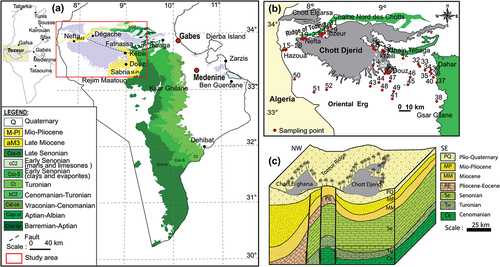
The Plio-Quaternary (PQ) shallow aquifer in Chott Djerid is a complex system that is composed of a variety of geological formations (Tarki, Dassi, & Jedoui, 2012). The main aquiferous units are the Quaternary alluvial deposits and the Pliocene sandstones and marls. PQ alluvial deposits are composed of sand, gravel, and clay. The overall thickness of reached 200 m in places (Kamel, Dassi, Zouari, & Abidi, 2005). Similarly, the Pliocene sandstones and marls reached 100 m thick series in the depressions and valleys of the Chott Djerid. PQ deposits lie uncomformably above the underlying formations of the well-known complex terminal (CT), represented by the Senonian fractured limestone and/or the Miocene Beglia and Segui sands (Figure 1).

Figure 1. Simplified geological map of southern Tunisia showing the study area (a), sampling points (b) and a bloc diagram (c) of the Chott Djerid aquifer system.

Materials and methods

Sampling

The sampling of 51 water samples from boreholes in the shallow aquifers of Djerid, Kebili, Douz, and Saharan area is a significant step in understanding water geochemical properties. Special attention was given to water points of the Chott Djerid shoreline and the adjacent Saharan aquifer because both areas are known to be vulnerable to water pollution. The assessment of geochemical characteristics is crucial in developing strategies to protect the water resources in this region. These areas are located in a desert climate, which means that the water is more likely to be contaminated by salts and other minerals. Moreover, these areas are also home to a number of cottage industries, which could be releasing pollutants into the water. In addition, the Chott Djerid is a large salt lake that can also be a source of pollution. Understanding water geochemistry in this region and identifying any potential problems can then be used to develop strategies to protect the water resources and ensure that they are safe for human consumption and other uses. This is fundamentally important for concerned stakeholders to develop policies to protect the water resources. Local communities should make informed decisions about their water use; businesses need to ensure that they are not polluting the water.

Sampling is a valuable first step in understanding the water properties to develop strategies for an integrated water resources management and ensure the safe human consumption and other uses. To this end, clean, sanitized water sample bottles, a disinfectant, and a pair of gloves were used during the collection of water samples. Water was first filtered through 0.45 µm pore size acetate filter. Then, in situ measurements of electric conductivity (EC), temperature (T) and pH were carried out immediately. Polypropylene bottles were carefully filled, tightly capped, labeled, and refrigerated at 4°C, before the delivery to the laboratory for subsequent analyses. Chemical analysis was performed as described by Kraiem et al. (2014). Briefly, bicarbonates were ascertained by titration, as described elsewhere (Bradbury & Baeyens, 2009). Major elements and nitrates concentrations were measured by a high performance liquid chromatograph equipped a Super-Sep column for anions.

Data preparation and preprocessing

The obtained data were subjected to a standardization step to have the same variation range that may allow an accurate application of neural network (i.e., BPNN). Data standardization is a pre-processing step to improve the performance of BPNN; it involves transforming the data to ensure same scale for all studied features. Z-score normalization was selected as it is generally preferred for tasks where the features are normally distributed (Akanbi, Amiri, & Fazeldehkordi, 2015; Corzo & Solomatine, 2007; Nazari, Taghavi, & Hajizadeh, 2021). Data standardization is an important step in preparing data for BPNN. It can help to improve the performance of the network, improve the convergence, and make the network easily interpretable.

Eq. (1) $Xn=2\ast \frac{X-Xmin}{Xmax-Xmin}-1$Eq. (1)

With Xn, X, Xmin, and Xmax are the standardized parameter, true parameter, minimum, and maximum of the studied parameter, respectively (Gholami, Moradzadeh, Maleki, Amiri, & Hanachi, 2014). Tidyverse is a set of R packages that were used for dataset pre-processing and presentation (Wickham et al., 2019). ggplot2 provided a complete implementation for graphical visualizations (Almeida, Loy, & Hofmann, 2019).

Cross validation metrics

For the sake of model accuracy and precision, multiple model evaluation criteria were used. To get a more complete picture of the model performance, the obtained results were compared for a realistic model validation. The size of the dataset (51 data points) was judged as plausible to satisfy a high accuracy of the prospective model. Based on preliminary investigations, data points are well prepared for the appropriate z-score normalization. A compromising model can ensure the desired accuracy since a complex model might be able to achieve higher accuracy than a simple model, but it might also be more prone to overfitting.

Root Mean Square Error (RMSE), Mean Squared Error (MSE), Sum of Squared Errors (SSE), coefficient of determination (R2), and Standard Deviation (SD) are all metrics used to evaluate the performance of the network (Kurtulus & Razack, 2010). They all measure the difference between the predicted values and the actual values, but they do so in different ways. RMSE is the most common metric used to evaluate regression models. It is calculated by taking the square root of the mean squared error (MSE). RMSE measures the average distance between the predicted values and the actual values. A lower RMSE indicates that the model is performing better. RMSE can be calculated as following:

Eq. (2) $RSME=\sqrt{\frac{\stackrel{n}{\sum _{i=1}}{(y_i-{\hat{y}}_i)}^2}{n}}$Eq. (2)

y_i and ŷ_i are the actual and predicted values, respectively. Mean squared error measures the average of the squared errors between the predicted values and the actual values. SSE is the sum of the squared errors between the predicted values and the actual values. SSE is a less sensitive measure of error than MSE, but it is easier to interpret. R² (coefficient of determination) is a measure of how well the model explains the variance in the data. R² can range from 0 to 1, with 1 indicating a perfect fit.

SD is a measure of the spread of the data. It is calculated by taking the square root of the variance. SD measures the average distance between the data points and the mean. A lower SD indicates that the data is more tightly clustered around the mean. It is generally recommended to use multiple metrics to evaluate model performance (Table 1).

Table 1. Summarized metrics used for model validation.

Metric	Formula	Description
RMSE	$\sqrt{MSE}$	Measures the average distance between the predicted and the actual values.	Eq. (1)Eq. (1) $Xn=2\ast \frac{X-Xmin}{Xmax-Xmin}-1$Eq. (1)
MSE	$\frac{\stackrel{n}{\sum _{i=1}}{(y_i-{\hat{y}}_i)}^2}{n}$	Average of the squared errors between the predicted and the actual values.	Eq. (2)Eq. (2) $RSME=\sqrt{\frac{\stackrel{n}{\sum _{i=1}}{(y_i-{\hat{y}}_i)}^2}{n}}$Eq. (2)
SSE	$\stackrel{n}{\sum _{i=1}}(y_i-{\hat{y}}_i{)}^2$	The sum of the squared errors between the predicted and the actual values.	Eq. (3)
R^2	$1-\frac{\sum _{i=1}^n{(y_i-{\hat{y}}_i)}^2}{\sum {(y_i-{\bar{y}}_i)}^2}$	Measures how well the model explains the variance in the data.	Eq. (4)
SD	$\frac{\stackrel{n}{\sum _{i=1}}{(y_i-{\bar{y}}_i)}^2}{n-1}$	Measures the spread of the data.	Eq. (5)

Multivariate statistical analyses

A set of statistical methods including principal component analysis (PCA), factor analysis (FA) and cluster analysis were applied as multivariate statistical tools to analyze the collected datasets with more than one independent variable and one dependent variable. PCA, FA and cluster analysis are the most common multivariate statistical analyses (Sahu et al., 2021). PCA is often used to identify the most important variables. Factor analysis may help to explain the covariation among the original variables. Cluster analysis was used for grouping water samples together based on their similarity (i.e. chemical composition). More detailed descriptions of those traditional statistical methods can be found in Kraiem et al. (2014).

Backpropagation neural network (BPNN)

Backpropagation neural networks (BPNNs) are trained using the backpropagation algorithm. The algorithm works by adjusting the weights of the connections between the nodes in the network. Those weights are adjusted so that the network learns to produce the desired output for a given input (Hameed et al., 2017). The backpropagation algorithm is an iterative process that starts by randomly assigning weights to the connections. Then, the network is presented with a training example. The output of the network is compared to the desired output, and the weights are adjusted accordingly. This process is repeated for a number of training examples until the network learns to produce the desired output for all of the training examples. The network converges when the error is minimized. Backpropagation algorithm is a powerful tool for training BPNN. However, many factors can affect the performance of a BPNN including the number of layers in the network, the number of nodes per layer, the learning rate, and the number of training examples. More layers and nodes can improve the performance of the network, but it can also make the network more computationally expensive to train (Zaresefat & Derakhshani, 2023). The learning rate is a parameter that controls how much the weights are updated in each iteration of the backpropagation algorithm. A high learning rate can make the network converge faster, but it can also make the network more prone to overfitting (Bashar, Nozari, Marofi, Mohamadi, & Ahadiiman, 2023; Tao et al., 2022; Zhu et al., 2022). The more training examples, the better the network will perform. Here, a large enough dataset was collected to run BPNN efficiently.

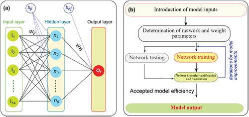
In summary, BPNN is a powerful tool for learning complex relationships between input and output data. In this work, 13 input neurons (physical and chemical properties), 1 hidden layer with 6 neurons and one output (TDS) were used for ANN model construction (Figure 2). Data points were split for train (80%) and test (20%) datasets for model training and evaluation. Back propagation algorithm was used for ANN training as it performs smoothly to provide faster convergence with a lower iteration number (Al-Mukhtar, 2021; Islam Khan, Islam, Uddin, Islam, & Nasir, 2022; Keskin et al., 2015; Zaqoot et al., 2018; Zhu et al., 2022).

Figure 2. (a) architecture of the ANN model used in this study and (b) the proposed predictive BP neural network model (modification after Bashar et al., 2023).

Results and discussions

Statistical summary of the studied groundwater samples of the PQ shallow aquifer of Chott Djerid was shown as mean, standard deviation (SD), median, minimum (Min), maximum (Max), range, skewness (Skew), kurtosis, and standard error (SE). Both kurtosis and skewness can highlight the distribution of a given hydrochemical parameter within the studied well points; they are classified as following:

• skew <0 – Left-skewness-extended left tail of the distribution

• skew = 0 – Symmetric distribution

• skew >0 – Right-skewness- extended right tail of the distribution

• leptokurtic (Kurtosis >0) – the distribution has a fatter tail (i.e. the intensity of extreme values is higher than in a normal distribution).

• mesocurtic (Kurtosis = 0) – the distribution is close to normal.

• platykurtic (Kurtosis <0) – the distribution has a thinner tail than the normal distribution (the intensity of extreme values is lower than in the normal distribution).

It appeared that EC varied between 535 and 13,330 µS/cm with a range of 12,795, median (7810 µS/cm) and a mean of 7052.2 µS/cm. This is an indication of left skewed and platykurtic dataset (Table 2). Similarly, total dissolved salts (TDS) and SO₄ exhibited almost same skewness and kurtosis. TDS varied between 360 and 11,010 mg/L with a mean of 5775.02 mg/L. NO₃ showed a mean of 40.93 mg/L, but much lower median (6 mg/L). This lead to an extended right tail of the distribution concomitantly with leptokurtic nature. This means that the distribution has a dominance of extreme values that are higher than in a normal distribution (i.e. flatter tail). The same behavior can be easily distinguished for CO₃, HCO₃ and K, but to a much lower extent. Mg varied between 16.39 and 477.81 mg/L with a symmetric distribution around the median and platykurtic kurtosis (i.e. dominance of low values). pH values extended over the interval [6.21–8.16] with a dominant acid-to circum-neutral values (Table 2).

Table 2. Statistical indexes of the studied water physical-chemical properties.

Var.	N	Mean	SD	Median	Min	Max	Range	Skew	Kurtosis	SE
Depth (m)	51	14.76	12.86	8.4	4.6	50	45.4	1.64	1.47	1.8
EC (µS/cm)	51	7052.2	3441.06	7810	535	13330	12795	−0.47	−0.75	481.84
Temp. (°C)	51	20.89	2.28	20.8	16	26.3	10.3	0.39	−0.08	0.32
pH	51	7.23	0.67	7.49	6.21	8.16	1.95	−0.37	−1.51	0.09
Cl (mg/L)	51	1495.83	986.75	1511.28	26.35	4179.7	4153.35	0.37	−0.2	138.17
NO3 (g/L)	51	40.93	98.31	6	0	558	558	4	16.5	13.77
SO4 (mg/L)	51	2021.31	959.95	2272.85	91.9	3482.8	3390.9	−0.82	−0.51	134.42
CO3 (mg/L)	51	3.54	9.4	0	0	42	42	2.68	6.44	1.32
HCO3 (mg/L)	51	273.78	175.18	268.4	25.62	895.48	869.86	1.34	2.57	24.53
Na (mg/L)	51	859.58	549.59	833.2	22.51	2277.6	2255.09	0.34	−0.32	76.96
K (mg/L)	51	49.16	51.39	49.9	0	253.04	253.04	1.92	4.78	7.2
Mg(mg/L)	51	243.27	141.46	256.2	16.39	494.2	477.81	−0.03	−1.1	19.81
Ca (mg/L)	51	613.38	264.67	697.65	41.07	1078.8	1037.73	−0.96	−0.07	37.06
Sr (mg/L)	51	4.8	3.74	4.61	0	10.88	10.88	0.1	−1.36	0.52
TDS (mg/L)	51	5775.02	2893.59	6260	360	11010	10650	−0.47	−0.73	405.18

Hierarchical cluster analysis and binary correlation

Hierarchical cluster analysis was used to reduce the data from the large number of individual water samples to smaller groups that have similar properties (Sherriff, Court, Johnston, & Stirling, 2002). Ward’s hierarchical agglomerative clustering method was used after centering and compiling the similarity matrix of Euclidian distance. The obtained dendrogram is a gathered presentation of water samples with similar and close geochemical properties. Cluster 1 (11 samples); Cluster 2 (23 samples), Cluster3 (6 samples) and Cluster4 (11 samples) were defined using a phenon line at a linkage of 10 (Figure 3).

Figure 3. Hierarchical cluster analysis of water samples from the Chott Djerid shallow aquifer.

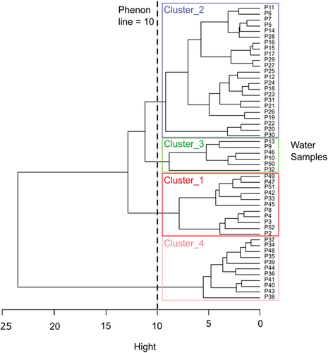
P2, P3, P4, P8, P33, P42, P45, P47, P49, P51, and P52 were attributed to Cluster 1 due to their similar chemical composition, especially calcium and magnesium contents. Calcium content varied between 405 and 808 mg/L while that of magnesium varied between 100 and 500 mg/L (Figure 4). An in depth examination of the cluster showed that most of those samples were collected from the oasis aquifers. Cluster 2 encompasses P5, P7, P11, P14, P15, P16, P17, P18, P19, P120, P21, P22, P23, P24, P25, P25, P28, P29, P30, and P31. Out of 23 samples, 17 water samples were collected from the same sub-aquifer (Djerid oasis). Thus, it was expected to have similar contents in Ca, Mg, HCO₃, SO₄ and NO₃. The remaining six samples (i.e., P5–7 from kebili and P11, P12, P14 from Douz) showed close similarity with regard to the same elements. Cluster 3, made up by P10, P13 (Douz) and P32, P42, P46 and P50 (Nefzaoua), were clustered due to the similar water temperature and pH, and Ca. Cluster 4 also grouped P34, P35, P36, P37, P38, P39, P40, P41, and P43. Surprisingly, all of those samples were collected from saharan aquifers. To conclude, clusters were split into 4 groups, mainly because of their origin (i.e., Djerid, Kebili, Douz, and Saharan regions). The spatial distribution is therefore an influencing factor of those waters geochemical characteristics. Similar observation was adopted by Abu Salem, Albadr, El Kammar, Yehia, and El-Kammar (2023) who integrated multivariate statistical analysis and hydrochemical modeling for the assessment of the main controlling processes that took place in Quaternary shallow aquifer (Beni Suef, Egypt). 

Figure 4. Boxplots for the studied geochemical parameters based on clusters.

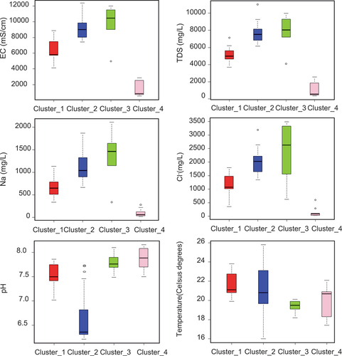
Figure 4. (Continued).

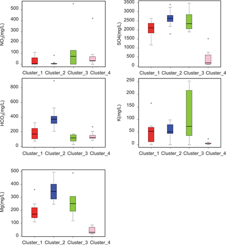
Pairs panels showed strong binary correlations of EC, Cl, SO₄, Na, Mg, Ca, and TDS (Figure 5). Correlation was considered significant when the coefficient of determination exceeded 0.7. The highest correlation was observed for TDS and EC (R² = 0.99). TDS was also highly correlated to Cl, SO₄, Na and Mg (R² ~0.93), indicating that those elements are the most influencing factors of water salinity. Ca was also positively correlated to TDS, but to a somewhat lower extent (R2 = 0.88). Both Na and Cl are strongly correlated to EC with R² values of 0.96 and 0.95, respectively, indicating their similar effects on EC and subsequently TDS. HCO₃, NO₃, CO₃, K, and Sr showed low correlation; they were removed from pairs panel (R² <0.7). Significant positive correlation between Na-Ca and Na-Mg indicated the prevalent contribution of the underlying lithology from which mineral dissolution dominated the geochemical process (Thomas, 2023).

Figure 5. Pairs panels for the studied geochemical parameters.

It is well known that the interaction of the groundwater with the hosting deposits (i.e. sands, clays, halite and gypsum) may grant a similar salinity as the host material (Kraiem et al., 2014), as the case of the present water samples. Khalfi, Tarki, and Dassi (2021) further indicated that PQ groundwater hydrochemistry was governed by fresh water and brines mixing process. However, they did not exclude the dissolution of MgSO₄ despite the insignificant correlation between Mg and SO₄ (R² = 0.6). This study confirmed a high relationship between both elements (R² = 0.89) as a further confirmation of MgSO₄ dissolution. Similarly, Ca and SO₄ showed almost the same coefficient of determination (R² = 0.88), probably due to gypsum and/or Chott brines intrusions.

Principal component analysis (PCA)

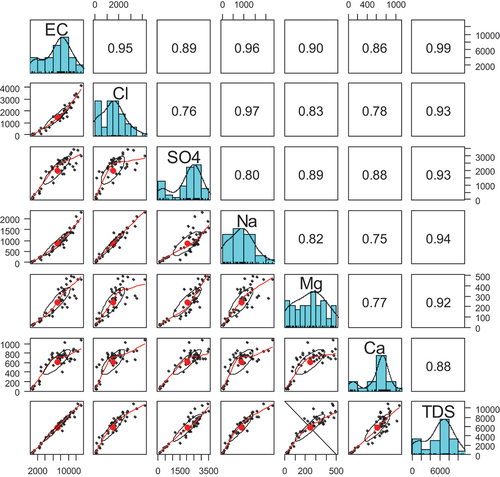
Principal component analysis (PCA) was performed on the raw data matrix of 14 variables (physico-chemical properties) and 51 individuals (total water samples). It was used, as a handy tool, to elucidate the main process underlying the geochemical composition of the studied shallow groundwater samples. PCA was performed by varimex rotation methodology to define the most influencing factors in groundwater geochemistry. The obtained results showed three predominant components (eigenvalue >1) with 82.674% of the cumulative variance (Figure 6, Table 3). The highest percentage of variance was observed for dimension 1 (Dim.1) with 61.06% (eigenvalue = 7.327). Dimension 2 exhibited 12.36% of variance (eigenvalue = 1.483), while dimension 3 reached 9.251% (eigenvalue = 1.110). These indices suggested that parameters like EC, TDS, Cl, Ca, SO₄, Mg are closely related due to geogenic sources of the elements. K, Na, HCO₃ and pH were associated with dimension 2 as a further confirmation of geogenic process behind which silicates weathering may alter the salinity values. Similar interpretation was given by Sahu et al. (2021) who ascertained groundwater contamination by fluoride. The last component (Dim. 3) suggested an anthropogenic source of NO₃, HCO₃ and CO₃ probably due to groundwater recharge processes and the effet of pasture (Sahu et al., 2021). An in-depth study of the collected groundwater samples may further shed light on the main chemical characteristics. Nitrate levels in the PQ water samples are contingent upon the irrigation practice, suggesting an infiltration along with nitrate-rich fertilizers. Groundwater properties are shaped by natural geogenic processes and, to a lower extent, by fertilizers addition during the flooding irrigation and the effect of grazing. this well confirm the explanation given by Kraiem et al. (2014) and Tarki et al. (2012) The latter proposed a conceptual model for groundwater salinization in which they suggested that return flow of irrigation water, application of fertilizers, and evaporation may further increase the salinity.

Figure 6. PCA variable factor map.

Table 3. Matrix of the main principal components and percentage of variance after variomax-rotation (n = 51).

Component
Parameter	1	2	3	4	5
EC	0.972	0.128	0.095	−0.118	0.037
Cl	0.902	0.126	0.159	−0.323	0.044
NO3	−0.194	0.787	−0.234	0.291	0.445
SO4	0.946	0.022	0.058	0.202	−0.022
CO3	−0.144	−0.126	0.844	0.481	0.051
HCO3	0.562	−0.59	−0.3	0.319	0.204
Na	0.92	0.195	0.086	−0.215	−0.012
K	0.548	0.55	−0.129	0.388	−0.454
Mg	0.938	−0.119	0.007	0.003	0.024
Ca	0.873	0.007	0.177	−0.025	0.179
TDS	0.989	0.074	0.072	−0.05	0.045
Sr	0.731	−0.327	−0.393	0.293	−0.053
Eigenvalue	7.327	1.483	1.11	0.863	0.49
Variance %	61.062	12.36	9.251	7.194	4.083
Cumulative %	61.062	73.422	82.674	89.868	93.951

Artificial neural network model

The architecture of BPNN, adopted here, included one hidden layer with 6 nodes (Figure 7). Preliminary trials have shown that models with 3 to 5 nodes did not give satisfactory results with regards to accuracy (less than 0.7), low sensitivity, and specificity. Thus, a six neurons layer has been found to achieve the highest fittings. Banerjee et al. (2011) evaluated the prospective use of ANN prediction to estimate a safe pumping rate that would maintain groundwater salinity in the desired threshold. They applied Feed-forward ANN model with back propagation algorithm to forecast the salinity under different conditions. They concluded that ANN model has emerged as a simple and accurate approach for predicting salinity. Minimal number of hidden neurons provided best performance over years. Guan and Yang (2020) focused on a back propagation neural network to monitor the leaching behavior of heavy metals in tea with the aim of improving health of consumers. They found that the constructed BPNN exhibited a fast convergence speed with an outstanding accuracy. BPNN, also called feedforward network, is a typical neural network being widely used for the prediction of a given output (Guan & Yang, 2020). The determination of neurons per hidden layer depended, mainly, on input and output variables. We aim to build a functional relationship between the salinity (expressed as TDS) and fourteen physicochemical parameters (i.e., EC, pH, Temperature, SO₄, NO₃, Na, Mg, Cl, K, HCO₃, CO₃, depth, Ca, Sr). To ovoid overfitting or insufficient ability to properly describe the output (i.e., TDS in mg/L), a compromising number of neurons per hidden layer was calculated based on the formula provided by Yin, Wang, and Yan (2011).

Eq. (3) $t=\sqrt{m+n}+i,0<i<10$Eq. (3)

Figure 7. Structure of the BPNN adopted in this study.

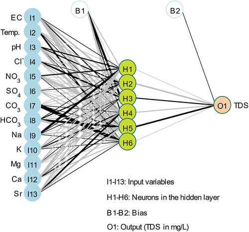
t: neurons in hidden layer; m: neurons in input layer; n: neurons in output layer i: number of samples used for training (40 water samples), but i takes 10 as stated in the formula. Overall flowchart of the adopted BPNN model is given in Figure 2. The prediction of TDS (mg/L) has been carried out via the relevant packages that allow a simple and convenient use of modeling facilities. Keskin et al. (2015) applied BPNN for the prediction of water pollution sources via the assessment of 13 water geochemical parameters, as the case in the current study. They reported that using more than one hidden layer is not required. Instead, variation of hidden nodes within the targeted layer may provide highly efficient results for BPNN model. Conjunction of Yin, Wang and Yan equation with the findings of Keskin et al. (2015) has oriented the modeling trials to 13:10:1 and 13:5:1 structure. Nevertheless, preliminary trials showed that a BPNN structure of 13:6:1 was the best to predict water salinity. Zhu et al. (2022) performed a comprehensive review of the application of machine learning in water quality evaluation. They focused on groundwater, among other application. It was stated that machine learning has emerged as an important tool for data analysis, classification, and prediction. This is the case for the present shallow groundwater samples.

Cross validation

The best cross-validation criterion for BPNN depends on the specific application, as the case of shallow groundwater salinity. In general, MSE and RMSE are good choices for regression problems, while R-squared and adjusted R-squared are good choices for evaluating the overall fit of the model. Surprisingly, the model has successfully predicted all testing dataset correctly with a very high accuracy, sensitivity, and specificity (Table 4). Pearson’s correlation coefficient between measured and predicted values was ascertained to 0.9940, further confirming an almost perfect fitting of the proposed BPNN model. Other cross validation criteria (RMSE, MSE, SSE, R², Adj R² and SD) also sustained the successful application of the model to predict groundwater salinity. In this work, the predicted and measured values well fitted a linear regression with a high coefficient of determination (R² = 0.9721) and low standard error (SE = 0.0546; Figure 8). Thus, it is suggested that the proposed BPNN has a great performance in predicting the Chott Djerid groundwater salinity. This is a further confirmation of the cross validation results (Table 4).

Figure 8. Fitting the predicted values from BPNN and experimental values.

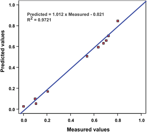
Table 4. Cross validation criteria for the proposed BPNN model.

Accuracy	Sensitivity	Specificity	Kappa	RMSE	MSE	SSE	R^2	Adj R^2	SD
1.0000	1.0000	1.0000	1.0000	0.0402	0.0016	0.0146	0.9721	0.9790	0.1240

In addition to the cross-validation criterion, other factors can affect the performance of BPNN (e.g., the number of hidden layers, the number of neurons in the hidden layer, the learning rate, and the activation function). These factors were controlled to optimize the performance of the model on the training set of data. The proposed model converged after 194 iteration steps, reaching the desired threshold (0.009).

Conclusions

This study has been carried out on water geochemical characteristics of the well-known Chott Djerid depression. The aim was a simulation/prediction of water salinity via the assessment of the TDS (mg/L) versus other influencing parameters (i.e., Na, K, Mg, Ca, EC, Cl, CO₃, HCO₃, Br, pH, temperature, depth, NO₃, SO₄). Those parameters were measured in situ and/or in the laboratory. The output was water salinity, expressed as TDS (mg/L). Salinization of groundwater is tightly related to various parameters including the host hydrogeochemical context of the Chott Djerid depression. Based on those physico-chemical properties, TDS was predicted by using BPNN model. The developed BP model has shown a high accuracy in the identification of the most influencing factor in groundwater salinity. Artificial neural network classification of water samples from Chott Djerid achieved more than 95% accuracy; it was successfully used as analytical tool to predict water salinity. The best performance was obtained with 6 neurons in the hidden layer. The obtained results showed that BPNN reached the required threshold of 0.009 (<0.01) that confirm the training accuracy. This highlighted the usefulness of BP neural network in predicting and simulating groundwater salinity. It provides an effective tool for water management in the Chott Djerid neighborhood.

Highlights

• Application of artificial neural network for salinity prediction

• Multivariate analysis of groundwater properties was performed

• A back propagation algorithm was successfully applied

• A high accuracy of ANN to predict groundwater salinity

• An effective tool for groundwater management was proposed

Author contributions

Zohra KRAIEM: Formal analysis, Writing – original draft, Writing – review & editing. Conceptualization, Methodology, Supervision, Data Curation, Visualization, Validation.

Kamel ZOUARI, Najiba CHKIR: Conceptualization, Methodology, Funding acquisition, Validation.

Acknowledgments

The authors extend their appreciation to Professor Zaher Mundher Yaseen from King Fahd University of Petroleum & Minerals for his active contribution to the proofreading of the manuscript.

Disclosure statement

No potential conflict of interest was reported by the author(s).

Data availability statement

Data are available upon request.

Supplemental material

Supplemental data for this article can be accessed online at https://doi.org/10.1080/23570008.2023.2294535

References

- Abu Salem, H. S., Albadr, M., El Kammar, M. M., Yehia, M. M., & El-Kammar, A. M. (2023). Unraveling the hydrogeochemical evolution and pollution sources of shallow aquifer using multivariate statistical analysis and hydrogeochemical techniques: A case study of the Quaternary aquifer in Beni Suef area, Egypt. Environmental Monitoring and Assessment, 195(670). doi:10.1007/s10661-023-11206-9
- Akanbi, O. A., Amiri, I. S., & Fazeldehkordi, E. (2015). Feature extraction. A mach. Approach to Phishing Detection and Defense, 45–54. doi:10.1016/B978-0-12-802927-5.00004-6
- Almeida, A., Loy, A., & Hofmann, H. (2019). ggplot2 compatible quantile-quantile plots in R. The R Journal, 10(2), 248. doi:10.32614/RJ-2018-051
- Al-Mukhtar, M. (2021). Modeling the monthly pan evaporation rates using artificial intelligence methods: A case study in Iraq. Environmental Earth Sciences, 80(1), 1–14. doi:10.1007/s12665-020-09337-0
- Al-Waeli, L. K., Sahib, J. H., & Abbas, H. A. (2022). ANN-based model to predict groundwater salinity: A case study of West Najaf–Kerbala region. Open Engineering, 12(1), 120–128. doi:10.1515/eng-2022-0025
- Banerjee, P., Singh, V. S., Chatttopadhyay, K., Chandra, P. C., & Singh, B. (2011). Artificial neural network model as a potential alternative for groundwater salinity forecasting. Canadian Journal of Fisheries and Aquatic Sciences, 398(3–4), 212–220. doi:10.1016/j.jhydrol.2010.12.016
- Bashar, A. M., Nozari, H., Marofi, S., Mohamadi, M., & Ahadiiman, A. (2023). Investigation of factors affecting rural drinking water consumption using intelligent hybrid models. Water Science & Engineering, 16(2), 175–183. doi:10.1016/J.WSE.2022.12.002
- Bradbury, M. H., & Baeyens, B. (2009). Sorption modelling on illite part I: Titration measurements and the sorption of Ni, co, Eu and sn. Geochimica Et Cosmochimica Acta, 73(4), 990–1003. doi:10.1016/j.gca.2008.11.017
- Corzo, G., & Solomatine, D. (2007). Knowledge-based modularization and global optimization of artificial neural network models in hydrological forecasting. Neural Networks, 20(4), 528–536. doi:10.1016/J.NEUNET.2007.04.019
- Dassi, L. (2011). Investigation by multivariate analysis of groundwater composition in a multilayer aquifer system from North Africa: A multi-tracer approach. Applied Geochemistry, 26(8), 1386–1398. doi:10.1016/j.apgeochem.2011.05.012
- Dhaouadi, L., Besser, H., Karbout, N., Wassar, F., & Alomrane, A. R. (2021). Assessment of natural resources in tunisian oases: Degradation of irrigation water quality and continued overexploitation of groundwater. Euro-Mediterranean Journal for Environmental Integration, 6(1), 1–13. doi:10.1007/s41207-020-00234-3
- Gholami, R., Moradzadeh, A., Maleki, S., Amiri, S., & Hanachi, J. (2014). Applications of artificial intelligence methods in prediction of permeability in hydrocarbon reservoirs. Journal of Petroleum Science & Engineering, 122, 643–656. doi:10.1016/J.PETROL.2014.09.007
- Guan, C., & Yang, Y. (2020). Research of extraction behavior of heavy metal cd in tea based on backpropagation neural network. Food Science and Nutrition, 8(2), 1067–1074. doi:10.1002/fsn3.1392
- Hameed, M., Sharqi, S. S., Yaseen, Z. M., Afan, H. A., Hussain, A., & Elshafie, A. (2017). Application of artificial intelligence (AI) techniques in water quality index prediction: A case study in tropical region, Malaysia. Neural Computing & Applications, 28(S1), 893–905. doi:10.1007/s00521-016-2404-7
- Islam Khan, M. S., Islam, N., Uddin, J., Islam, S., & Nasir, M. K. (2022). Water quality prediction and classification based on principal component regression and gradient boosting classifier approach. Journal of King Saud University - Computer and Information Sciences, 34(8), 4773–4781. doi:10.1016/J.JKSUCI.2021.06.003
- Jamei, M., Karbasi, M., Malik, A., Abualigah, L., Islam, A. R. M. T., & Yaseen, Z. M. (2022). Computational assessment of groundwater salinity distribution within coastal multi-aquifers of Bangladesh. Scientific Reports, 12(1), 1–28. doi:10.1038/s41598-022-15104-x
- Kamel, S., Dassi, L., Zouari, K., & Abidi, B. (2005). Geochemical and isotopic investigation of the aquifer system in the Djerid-Nefzaoua basin, southern Tunisia. Environmental Geology, 49(1), 159–170. doi:10.1007/s00254-005-0076-1
- Keskin, T. E., Düğenci, M., & Kaçaroğlu, F. (2015). Prediction of water pollution sources using artificial neural networks in the study areas of sivas, Karabük and Bartın (Turkey). Environmental Earth Sciences, 73(9), 5333–5347. doi:10.1007/s12665-014-3784-6
- Khalfi, C., Tarki, M., & Dassi, L. (2021). An appraisal of Chott El jerid brine encroachment in the Tozeur-south shallow aquifer: Geoelectrical and hydrochemical approach. Journal of Applied Geophysics, 190, 104341. doi:10.1016/j.jappgeo.2021.104341
- Khudhair, Z. S., Zubaidi, S. L., Al-Bugharbee, H., Al-Ansari, N., & Ridha, H. M. (2022). A CPSOCGSA-tuned neural processor for forecasting river water salinity: Euphrates river, Iraq. Cogent Engineering, 9(1). doi:10.1080/23311916.2022.2150121
- Kraiem, Z., Zouari, K., Chkir, N., & Agoune, A. (2014). Geochemical characteristics of arid shallow aquifers in Chott Djerid, south-western Tunisia. Journal of Hydro-Environment Research, 8(4), 460–473. doi:10.1016/j.jher.2013.06.002
- Kurtulus, B., & Razack, M. (2010). Modeling daily discharge responses of a large karstic aquifer using soft computing methods: Artificial neural network and neuro-fuzzy. Canadian Journal of Fisheries and Aquatic Sciences, 381(1–2), 101–111. doi:10.1016/J.JHYDROL.2009.11.029
- Nazari, H., Taghavi, B., & Hajizadeh, F. (2021). Groundwater salinity prediction using adaptive neuro-fuzzy inference system methods: A case study in Azarshahr, Ajabshir and Maragheh plains, Iran. Environmental Earth Sciences, 80(4), 1–10. doi:10.1007/s12665-021-09455-3
- Rani, R. D., & Sasidhar, P. (2011). Stability assessment and characterization of colloids in coastal groundwater aquifer system at Kalpakkam. Environmental Earth Sciences, 62(2), 233–243. doi:10.1007/s12665-010-0517-3
- Sabzevar, M. S., Rezaei, A., & Khaleghi, B. (2021). Incremental adaptation strategies for agricultural water management under water scarcity condition in northeast Iran. Regional Sustainability, 2(3), 224–238. doi:10.1016/J.REGSUS.2021.11.003
- Sahu, S., Gogoi, U., & Nayak, N. C. (2021). Groundwater solute chemistry, hydrogeochemical processes and fluoride contamination in phreatic aquifer of Odisha, India. Geoscience Frontiers, 12(3), 101093. doi:10.1016/j.gsf.2020.10.001
- Sherriff, B. L., Court, P., Johnston, S., & Stirling, L. (2002). The source of raw materials for roman pottery from Leptiminus, Tunisia. Geoarchaeology: An International Journal, 17(8), 835–861. doi:10.1002/gea.10043
- Stivaletta, N., Barbieri, R., Picard, C., & Bosco, M. (2009). Astrobiological significance of the sabkha life and environments of southern Tunisia. Planetary & Space Science, 57(5–6), 597–605. doi:10.1016/j.pss.2008.10.002
- Tao, H., Hameed, M. M., Marhoon, H. A., Zounemat-Kermani, M., Salim, H. … Mehr, A. D. (2022). Groundwater level prediction using machine learning models: A comprehensive review. Neurocomputing, 489, 271–308. doi:10.1016/j.neucom.2022.03.014
- Tarki, M., Dassi, L., & Jedoui, Y. (2012). Groundwater composition and recharge origin in the shallow aquifer of the Djerid oases, southern Tunisia: Implications of return flow. Hydrological Sciences Journal, 57(4), 790–804. doi:10.1080/02626667.2012.681783
- Thomas, E. O. (2023). Evaluation of groundwater quality using multivariate, parametric and non-parametric statistics, and GWQI in Ibadan, Nigeria. Water Science, 37(1), 117–130. doi:10.1080/23570008.2023.2221493
- Wickham, H., Averick, M., Bryan, J., Chang, W., McGowan, L. … Yutani, H. (2019). Welcome to the Tidyverse. Journal of Open Source Software, 4(43), 1686. doi:10.21105/joss.01686
- Yebdri, L., Hadji, F., Harek, Y., & Marok, A. (2021). Quality assessment of water used for human consumption and irrigation purpose in parts of Tafna watershed (NW Algeria). Environmental Earth Sciences, 80(16), 1–15. doi:10.1007/s12665-021-09805-1
- Yin, Y. H., Wang, C. F., & Yan, M. Y. (2011). BP neural network in predicting the nano‐titanium dioxide photocatalytic degradation of nitrotoluene wastewater. Chinese Journal of Explosives & Propellants, 34(3), 86–90.
- Zaqoot, H. A., Hamada, M., & Miqdad, S. (2018). A comparative study of ANN for predicting nitrate concentration in groundwater wells in the southern area of gaza strip. Applied Artificial Intelligence, 32(7–8), 727–744. doi:10.1080/08839514.2018.1506970
- Zaresefat, M., & Derakhshani, R. (2023). Revolutionizing groundwater management with hybrid AI models: A practical review. Water (Switzerland), 15(9), 1750. doi:10.3390/w15091750
- Zhu, M., Wang, J., Yang, X., Zhang, Y., Zhang, L., … Ye, L. (2022). A review of the application of machine learning in water quality evaluation. Eco-Environment & Health, 1(2), 107–116. doi:10.1016/j.eehl.2022.06.001