Comparative analysis of classification techniques and input-output patterns for monthly rainfall prediction

ABSTRACT

Rainfall prediction is one of the crucial stages of the watershed management process. In this research, A comparison of the performance among Monte Carlo and Thomas Fiering, linear regression (LR), multiple linear regression (MLR), and SVM optimized by Simulated Annealing (SVM-SA) is carried out for Monthly rainfall prediction. In addition, the efficiency of the input patterns to the models including single input-multiple output (SIMO), multiple input-multiple output (MIMO), single input-single output (SISO), multiple input-single output (MISO) patterns are investigated. For this purpose, the time series of 34 rain gauge stations in the Karkheh basin was used. The results showed that SISO, MISO, MIMO, SIMO, and Monte Carlo and Thomas Fiering models are ranked first to fifth respectively. By comparing the performance of the models, it can be found that there is no significant difference between the SVM-SA, LR, and MLR models, However, the LR model is a method for predicting monthly rainfall more easily than other methods. This method has fewer adjustable parameters than other models.

KEYWORDS:

• Artificial intelligence
• prediction
• rainfall
• support vector machine

Introduction

One of the most important environmental issues now is the water crisis. It has environmental, social, and economic impacts. Several factors such as population growth, the limitation of freshwater resources, water quality reduction, and floods and droughts have made the need to act even more urgent, and use appropriate strategies for managing water resources (Giang, Wang, Hieu, Phuong, & Thinh, 2022). In this regard, accurate determination of hydrological parameters, e.g. rainfall has a major contribution to water resources management.

It is difficult to model and predict rainfall because of its spatial and temporal changes and uncertainty (Parmar, Mistree, & Sompura, 2017). On the other hand, reconstructed time series are essential to predict hydrological parameters that are constantly changing (Arriagada, Dieppois, Sidibe, & Link, 2019). Therefore, rainfall predicting is also done with models, such as numerical models connected to meteorological radar data, including multiple regression models and climatology models (Shao & Li, 2013; Tanessong, Igri, Vondou, Tamo, & Kamga, 2014), empirical formulas (Silvestro & Rebora, 2014) and numerical methods (Azadi, Taghizadeh, Memarian, & Dmitrieva-Arrago, 2013; Novak et al., 2014). In recent years, the use of classical models and artificial intelligence in the field of water resources and predicting hydrological parameters has been welcomed by many researchers. Classical models, e.g. Monte Carlo and Thomas Fiering, and Artificial intelligence models, e.g. neural network (ANN), genetic programming (GP), multiple linear and non-linear regression models, and support vector machine (SVM) and meta-heuristic algorithms, are usually used in hydrological parameter prediction studies (Choubin, Khalighi-Sigaroodi, Malekian, & Kis¸i, 2016; Danandeh Mehr, Nourani, Karimi Khosrowshahi, & Ghorbani, 2019; Lin, Zhang, Zhou, & Shen, 2022; Safari, Rahimzadeh Arashloo, & Danandeh Mehr, 2020).

Reddy, Yadala, and Goddumarri (2022) utilized the Singular-Spectrum-Analysis (SSA) technique in combination with the Least-Squares Support Vector Regression (LS-SVR) and Random-Forest (RF) models to predict and assess monthly rainfall. Their findings demonstrated that the proposed model, with a Root Mean Square Error (RMSE) of 71.6% and Nash – Sutcliffe Efficiency (NSE) of 90.2%, exhibits strong performance in rainfall forecasting. Abebe and Endalie (2023) recognized the significance of rainfall prediction in long-term decision-making and multiple planning, as well as the growing role of artificial intelligence in forecasting hydrological parameters. They employed Artificial Neural Networks (ANN) and Adaptive Neuro-Fuzzy Inference System (ANFIS) to predict monthly rainfall for 92 Ethiopian meteorological stations. Their findings indicated that the ANFIS model outperformed the ANN model in all stations. Markuna et al. (2023) examined four models, namely Multiple Linear Regression (MLR), Support Vector Regression (SVR), Multivariate Adaptive Regression Splines (MARS), and Random Forest (RF), for predicting daily and weekly rainfall in the Uttarakhand region. The results ranked the models as RF, MARS, SVR, and MLR in terms of performance, with RF being the top performer and MLR being the least effective. However, the SVM is one of the models based on supervised learning algorithms, which has been welcomed by researchers for classification and regression. One of the advantages of this model is simple training and not getting stuck in local extreme points. Due to its robustness and generalization performance, this model has been used to increase the accuracy of monthly rainfall predicts (Du, Liu, Yu, & Yan, 2017). Dawoodi (2021) utilized the SVM model to predict rainfall in three districts of the North Maharashtra region. They incorporated 16 meteorological parameters, such as temperature, wind speed, and humidity, as inputs, with rainfall as the output. The results show that the model achieved an 82% accuracy in forecasting monthly rainfall. In another study, Abdullah, Ruchjana, Jaya, and (2021) employed SARIMA and SVM models to forecast rainfall for the establishment of early warning systems aimed at detecting massive floods in Indonesian cities. Their focus on accurate rainfall prediction led to the conclusion that the SVM model offers more precise results. Moharana, Sahoo, and Ghose (2022) conducted a study to forecast rainfall in the Cachar region of India. They introduced a combined model of SVM and Harris Hawks Optimization (SVM-HHO). The results of this research validate that the hybrid model demonstrates strong generalizability and increased accuracy in monthly rainfall prediction. Kisi and Cimen (2012) used the combined wavelet-SVM model to predict precipitation. Ortiz-García, Salcedo-Sanz, and Casanova-Mateo (2014) used a set of predictive variables to predict daily precipitation and analyzed the importance of humidity and equivalent potential temperature variables using the SVM model. The results showed SVM had excellent performance compared to K-nearest neighbor and multilayer perceptron (MLP). Pham et al. (2020), used artificial neural network models (ANN), support vector machine (SVM) and adaptive neuro fuzzy inference system optimized with particle swarm optimization (PSOANFIS) to predict daily rainfall and found that SVM was the most powerful and efficient model. Moreover, various studies have shown that the SVM model can be used for classification and prediction, with high accuracy using data mining techniques based on machine learning (Hamidi et al., 2015; Nozari & Tavakoli, 2020; Sehad, Lazri, & Ameur, 2017; Shenify et al., 2016; Tao et al., 2018; Zaini, Malek, Yusoff, Mardi, & Norhisham, 2018). On the other hand, in recent years, researchers used different techniques to determine which algorithm or structure gives the best prediction. Patra, Mitra, and Pinchera (2020) has used the multiple input-multiple output (MIMO) technique to the proposed communication link model designed for 5 G communication in tropical regions. To interpret hydrological processes, Galelli and Castelletti (2013) applied the tree algorithm to determine the best input and output structures, such as single input-single output (SISO) and multiple input-single output (MISO). Amisigo, Van de Giesen, Rogers, Andah, and Friesen (2008); Nasir and Weyer (2016) used SISO, MIMO, and MISO techniques to predict hydrological parameters.

The aim of the current study is to evaluate different input and output patterns to check the performance of selected models in predicting monthly rainfall. For this purpose, support vector machine models combined with Simulated annealing algorithm (SVM-SA), linear regression (LR) and multiple linear regression (MLR) models, and input and output patterns, including single input-multiple output (SIMO), multiple input-multiple output (MIMO), single input-single output (SISO) and multiple input-single output (MISO) were used. In fact, the main goal of the authors for the application of different input and output patterns is to check the performance accuracy of the used models and compare it with the classic Monte Carlo and Thomas Fiering models and to introduce the best model for researchers to use in order to predict monthly rainfall.

Methodology

Study area

The Karkheh watershed is located in southwestern Iran and is one of the largest and most important river basins in the country. It covers an area of approximately 52,000 square kilometers and is named after the Karkheh River, which flows through the region. Also, its height varies from 80 meters (south of the basin) to 3598 meters (northeast) (Rahimi, Arian, & Ghorashi, 2017). The Karkheh River originates from the Zagros Mountains and serves as a vital water source for both agricultural and domestic purposes in the surrounding areas. It plays a crucial role in supporting irrigation, hydropower generation, and providing water for drinking and industrial use.

The watershed is characterized by diverse ecosystems, including forests, wetlands, and agricultural lands. It is home to a variety of plant and animal species, making it ecologically significant. The region’s natural resources and biodiversity contribute to its ecological value and provide opportunities for tourism and recreational activities. However, the Karkheh watershed also faces challenges related to water management and sustainability. Due to increasing water demands, climate change, and inadequate infrastructure, there are concerns about water scarcity, droughts, and environmental degradation in the region. Overall, the Karkheh watershed in Iran is an important natural resource that supports various sectors and ecosystems. Its sustainable management is crucial for ensuring water availability, preserving biodiversity, and supporting the livelihoods of the communities that depend on it.

The stations selected and studied in this research include 34 rain gauge stations located in the Karkheh catchment area. These rain gauge stations are strategically positioned throughout the watershed to capture precipitation data and provide insights into the hydrological processes within the Karkheh River basin. The distribution of these rain gauge stations ensures comprehensive coverage of the Karkheh catchment area, allowing researchers to gather accurate and representative data on rainfall patterns and amounts across the region. The data from the mentioned rain gauge stations was received from the Iranian Water Resources Management Company (Iranian Water Resources Management Company, 2022). Figure 1 shows the location, and Table 1 shows the characteristics of these stations. In the following, due to the increase of the studied stations, the results of the performance of different models in the 10 selected stations specified in Table 1 will be investigated. Figure 2 displays the time series of observed rainfall from several rain gauge stations in the basin, providing insight into the region’s rainfall variations.

Figure 1. Geographical location of karkheh basin and selected rainfall stations.

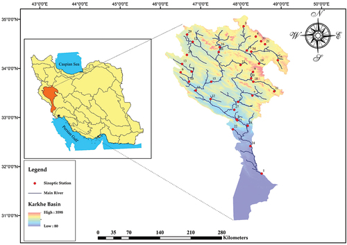
Figure 2. Rainfall time series in the rain gauge stations of Sarab Seyed Ali, Kaka Reza, Afrine (kashkan) and Pol Dokhtar.

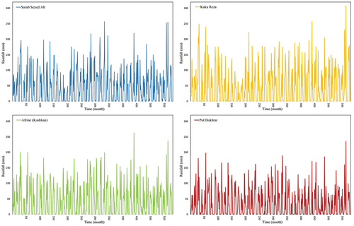
Table 1. Characteristics of selected synoptic stations in the Karkhe basin.

Row	Station name	Height	Longitude	Latitude	Row	Station name	Height	Longitude	Latitude
1	Abdolkhan	40	48.38	31.83	18	Kaka Reza	1530	48.25	33.71
2	Afrine (Kashkan)	800	47.87	33.31	19	Kanal Varayene	1759	48.4	34.08
3	Aghajan Bolaghi	1802	48.05	34.85	20	Kashenbele Lak	46.64	34.29	1500
4	Baba Pir Ali	1917	48.35	34.63	21	Kheir Abad	1770	48.57	34.47
5	Badr Gard	1274	46.75	33.95	22	Murmuri	485	47.72	32.75
6	Baskele Boorim	1460	46.48	33.94	23	Noor Abad	1780	47.95	34.06
7	Cham Anjir	1140	48.22	33.43	24	Pay Pol	125	48.13	32.4
8	Cham Gaz	385	47.82	32.95	25	Pihan	1820	48.87	34.13
9	Dare Tang Alashtar	1720	48.25	33.91	26	Pol Chehr	1280	47.43	34.34
10	Dartoot	1110	46.68	33.74	27	Pol Dokhtar	700	47.77	33.15
11	Dehno (Herood)	1800	48.75	33.5	28	Pol Zal	335	48.08	32.82
12	Doab Merk	1310	46.79	34.55	29	Ravansar	1343	46.65	34.7
13	Eslam Abad	1349	46.52	34.11	30	Sarab Seyed Ali	1520	48.2	33.78
14	Firoozan	1503	48.12	34.35	31	Sarabi	1925	48.48	34.53
15	Halilan (Simereh)	1000	47.23	33.73	32	Tang Siab	880	47.2	33.38
16	Heidar Abad	1290	47.45	34.43	33	Vargach	703	46.84	33.56
17	Jelogir	370	47.83	32.93	34	Vesaj	1650	48.22	34.32

Support vector machine (SVM) model

In 1965, Vladimir Vapnik presented the Support Vector Machine (SVM) model based on statistical theory. This model is based on binary classification in the space of arbitrary features, and hence it is considered a suitable method for predicting problems (Pai & Hong, 2007). Dibak presented the first application of this model in the field of hydrological parameters in predicting rainfall and runoff. This model is a relationship between dependent (y) and independent values in a given function f with an additional value whose purpose is to find the structure of the f function for correct prediction. It can be concluded that SVM is an efficient learning system that simultaneously minimizes the complexity of the model and also uses the inductive principle of standard error minimization to reach an optimal solution (Benimam, Si-Moussa, Laidi, & Hanini, 2020).

The SVM model has two key features: excellent generalization and compatibility with sparse data, leading to accurate predictions (Behzad, Asghari, & Coppola, 2010). This technique has two types, regression of the first type and regression of the second type, shown as SVM-ν and SVM-ɛ, respectively. The second type is more applicable in regression problems, and this model minimizes the error function Eq. (1) by considering a series of restrictions Eq. (2) (Ahmadi, Radmanesh, & Mir Abbasi Najafabadi, 2013).

Eq. (1) $\frac{1}{2}{W}^T\mathit{W}+\mathit{C}{\sum }_{i=1}^N{\mathit{\xi }}_{\mathrm{i}}+\mathit{C}{\sum }_{i=1}^N{\xi }_{\mathrm{i}}^{\ast }$Eq. (1)

Eq. (2) $W^T\mathit{\varphi }\left(x_i\right)+\mathit{b}-y_i\le \mathit{\epsilon }+{\xi }_{\mathrm{i}}^{\ast },\text{break}{y}_i-W^T\mathit{\varphi }\left(x_i\right)-\mathit{b}\le \mathit{\epsilon }+{\xi }_{\mathrm{i}}^{\ast },\text{break}{\xi }_{\mathrm{i}}^{\ast },{\mathit{\xi }}_{\mathrm{i}}\ge 0$Eq. (2)

Here, C is the capacity constant, w is the vector of coefficients, b is the constant, and ξi represents parameters for handling non-separable data (inputs). The Index i labels the N training items. The kernel ϕ is used to transform data from the (independent) input to the feature space (Nozari & Tavakoli, 2020).

This model can solve non-linear problems by changing the dimensions of the problem using the kernel. In practice, there are four types of kernels, the selection of the appropriate kernel depends on the amount of training data and the dimensions of the feature vector, but many hydrological studies are conducted based on the RBF kernel (Yu, Chen, & Chang, 2006). The names and mathematical equations of these nuclei are presented in Table 2. In these equations, γ and C are the parameters related to the kernel, and d is the polynomial degree.

Table 2. Types of kernel functions (Ren, Hu, & Miao, 2016).

Kernel	Formula	Optimization Parameter(s)
Linear	$\mathrm{K}\left({\mathrm{x}}_{\mathrm{i}}.{\mathrm{x}}_{\mathrm{j}}\right)={\mathrm{x}}_{\mathrm{i}}\ast {\mathrm{x}}_{\mathrm{j}}$	-
Polynomial	$\mathrm{K}\left({\mathrm{x}}_{\mathrm{i}}.{\mathrm{x}}_{\mathrm{j}}\right)={\left(\mathit{\gamma }\left({\mathrm{x}}_{\mathrm{i}}\ast {\mathrm{x}}_{\mathrm{j}}\right)+\mathrm{C}\right)}^{\mathrm{d}}$	$\mathit{\gamma }.\mathrm{C}.\mathrm{d}$
Hyperbolic tangent	$\mathrm{K}\left({\mathrm{x}}_{\mathrm{i}}.{\mathrm{x}}_{\mathrm{j}}\right)=\tanh \left(\mathit{\gamma }{\mathrm{x}}_{\mathrm{i}}\ast {\mathrm{x}}_{\mathrm{j}}+\mathrm{C}\right)$	$\mathit{\gamma }.\mathrm{C}$
RBF	$\mathrm{K}\left({\mathrm{x}}_{\mathrm{i}}.{\mathrm{x}}_{\mathrm{j}}\right)=\exp \left(-\mathit{\gamma }{\left|{\mathrm{x}}_{\mathrm{i}}-{\mathrm{x}}_{\mathrm{j}}\right|}^2\right)$	$\mathit{\gamma }$

Simulated annealing (SA) algorithm

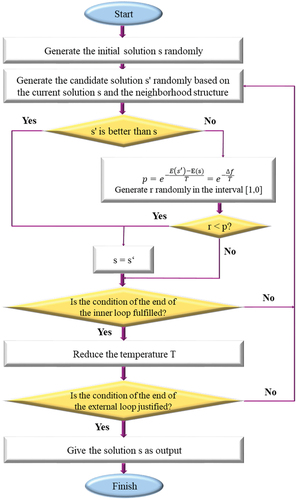
SA is a probabilistic meta-heuristic method based on the Monte Carlo model presented by Metropolis and his colleagues in 1953. Despite its simple structure, it effectively soles combinatorial optimization problems. The basis of this algorithm is based on the relationship between the atomic structure, entropy, and temperature during a substance’s cooling and on the physical phenomenon of annealing (Tran & Tran, 2007). SA is a local search method that seeks the optimal global solution. It solves optimization problems that include many independent variables due to its simplicity and efficiency. This algorithm starts with from an initial solution and then moves to neighboring solutions in an iteration loop. If the neighboring answer is better than the current one, the algorithm places it as the current one. In the early stages, the temperature is set too high to be more likely to accept more unfavorable solutions. As several iterations are run at each temperature, the temperature is slowly lowered. So with the gradual temperature decrease in the final steps, there will be less possibility of accepting unfavorable answers. As a result, the algorithm converges toward the desired and optimal solution (Rosen & Harmonosky, 2005).

The simulated refrigeration algorithm uses the Boltzmann probability distribution (Cercignani, 1988), which can be seen in Eq. (3), where E and T represent the energy and temperature of the system, respectively, and kb represents the Boltzmann constant. This distribution emphasizes that when a system is in thermal equilibrium at temperature T, it also has an energy distribution that is distributed among all the different energy states. It is possible to have a high energy state even at a low system temperature.

Eq. (3) $\mathrm{P}\left(\mathrm{E}\right)\propto \exp \left(-\mathrm{E}/{\mathrm{k}}_{\mathrm{b}}\mathrm{T}\right)$Eq. (3)

One of the essential advantages of this algorithm is that, unlike local optimization methods that can only find a minimum value close to the initial guess, the SA method can find the absolute minimum value. Sometimes it is better to return to an answer that has already been found than to make a move from the current state (Tran & Tran, 2007). In Figure 3, the general structure of the SA algorithm can be seen.

Figure 3. The general structure of the SA algorithm.

Support vector machine model based on SA algorithm (SVM-SA)

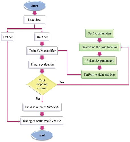
In recent years, many studies have been done to optimize the parameters of the SVM model, and researchers and experts recommended many methods. Research (Subasi, 2013) proposed a particle swarm optimization algorithm to optimize the parameters of the SVM model. Another study (Zhang, Chen, & He, 2010) used the ant colony optimization algorithm (ACO) for this purpose. The research results showed that the ACO algorithm could not optimize optimal solutions. The ACO algorithm also easily gets stuck in the local optimum due to its low convergence speed. Also, the GA algorithm has a low search speed because it must be decoded first and then decoded. The SA algorithm is used in this article to optimize the parameters of the SVM model, to solve these problems. The steps of implementing the SA algorithm in the SVM model are summarized as follows:

1. Unprocessed original data is imported to train the model.

2. Data processing and segmentation take place in the model.

3. SA algorithm is executed to find the optimal solution.

4. The data of the validation section is entered into the model, and the classification results are obtained.

In Figure 4, the flow structure of the SVM-SA model can be seen.

Figure 4. Flow structure of SVM-SA model (Bashar, Nozari, Marofi, Mohamadi, & Ahadiiman, 2023).

Linear regression (LR) and multiple linear regression (MLR) model

Linear regression (LR) is one of the oldest statistical models that has been widely used to analyze hydrological data (Stanton & Galton, 2001; Yan & Su, 2009). In fact, in this model, the relationship between the dependent and independent variables is assumed to be linear, and this model measures the effect of the independent variable on the dependent variable and examines the correlation between them. In this research, the ordinary least squares method was used, in which linear regression is calculated in such a way that there is the least sum of squares between the measured and predicted values (Park et al., 2020).

Different linear regression models include simple linear, logistic, polynomial, and multivariate linear regression (Kisi & Ozkan, 2017). Multiple linear regression (MLR) has been more widely used due to its simple formulation (Wang, Shangguan, Wu, & Guan, 2013). In multivariable linear regression, the parameters of a linear model are estimated with the help of an objective function and variable values. The way linear regression works is expressed as Eq. (4) where x₁, x₂, … and x_n are independent variables, and b₀, b₁, b₂, … and b_n are constant coefficients:

Eq. (4) $\mathit{Y}=b_0+b_1{x}_1+b_2{x}_2+\dots +b_n{x}_n$Eq. (4)

In this research, CORREL model was used for prediction with the help of linear regression model and SPSS software was used for prediction with the help of multiple linear regression model.

The relationship between the independent and dependent variables is expressed in simple linear regression as a line equation. In multiple regression, if two independent variables are in a linear relationship with a dependent variable, the shape of this relationship will be a plane. If more than two independent variables are used in the linear regression model, the model appears as a “hyperplane.”

Thomas Fiering model

The Thomas Fiering model is one of the time series models for predicting based on the Markov chain. The model incorporates seasonality into data variability by analyzing monthly fluctuations in average values and correlation coefficients (Sh, Khan, & Parida, 2001). In this model, the amount of the parameter in the coming months is obtained using past statistical data and a random variable based on the normal probability distribution function. In fact, in this method, each independent data is dependent on the data of the previous month, and in general, the governing equation is expressed as Eq. (5) (Arselan, 2012):

Eq. (5) $x_j={\bar{x}}_{\mathit{j}}+b_j\left(x_{\mathit{j}-1}-{\bar{x}}_{\mathit{j}-1}\right)+t_i{\sigma }_j{\left(1-r_{j.j-1}^2\right)}^{0.5}$Eq. (5)

In this relationship, x is the amount of rainfall or runoff, ${\bar{x}}_{\mathit{j}}$ is the average rainfall or runoff, σ is the standard deviation of rainfall or runoff values, $t_i$ is the standard normal number with a mean of zero and a variance of one, and j represents the month. The coefficient $b_j$ is calculated as Eq. (6), where r is the correlation coefficient.

Eq. (6) $b_j=r_{\mathit{j}.\mathit{j}-1}\frac{{\mathit{\sigma }}_{\mathit{j}-1}}{{\sigma }_j}$Eq. (6)

Definitions of input and output system types

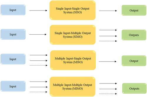
A system of inputs and outputs can be described as one of four types: single input-multiple output (SIMO), multiple input-multiple output (MIMO), single input-single output (SISO), and multiple input-single output (MISO).

These structures can be understood as follows:

1. SISO: SISO machine learning systems have a single input and a single output. This is the basic configuration for many traditional machine learning models, such as simple linear regression

In this study, the input pattern for determining SISO involved using the statistics of nearby stations as independent stations with a high correlation percentage and a close distance of 34 dependent stations. Furthermore, the model incorporated introducing the monthly rainfall timeseries of independent stations into the model based on the order of occurrence time as input and introducing the monthly rainfall timeseries of dependent station in the order of occurrence time as output.

2. SIMO: In SIMO machine learning systems, there is a single input and multiple outputs. This can be seen in scenarios such as regression models where multiple predictions are made based on a single input.

In the current study, the SIMO model utilized the annual rainfall data of all 34 stations as input, and introduced the 12-month rainfall statistics of the same station as the output of the model.

3. MISO: In MISO machine learning systems, there are multiple inputs and a single output. This can be observed in tasks where multiple features are used to predict a single target variable, such as in some types of regression or forecasting models.

In the present study, the MISO model utilized the time series data of three stations to forecast and reconstruct monthly rainfall. Two stations’ time series data were used as independent, while one station’s data was used as dependent. Due to the absence of three highly correlated and closely located stations, the rainfall data of 18 rain gauge stations were reconstructed and predicted. The model took the monthly rainfall data of independent and affiliated stations based on the order of occurrence time as input and output, respectively.

4. MIMO: MIMO machine learning systems involve multiple inputs and multiple outputs. This is common in tasks such as multi-label classification or when making predictions based on multiple input features.

In this study, time series data from adjacent stations, designated as independent stations, were used in pairs. These independent stations were selected based on high correlation with the dependent station and proximity in distance. The 12-month rainfall data of the independent station was used as input, while the 12-month rainfall data of the associated station was used as output for the model.

The schematic diagram of these systems is shown in Figure 5.

Figure 5. Structure of four machine learning systems: SISO, SIMO, MISO and MIMO.

Validation of the model

In this research, to evaluate and validate the results of the models in the reconstruction and predicting of rainfall, statistical indicators of root mean square error (RMSE), standard error (SE), Nash – Sutcliffe efficiency coefficient (NSE), and coefficient of determination (R²) were used. (Azadi, Nozari, & Godarzi, 2020)

Eq. (7) $\mathit{RMSE}=\sqrt{\frac{{\sum }_{i=1}^n{\left(Y_m-Y_p\right)}^2}{\mathit{n}}}$Eq. (7)

Eq. (8) $\mathit{SE}=\frac{\sqrt{\frac{1}{n}{\sum }_{i=1}^n{\left(Y_m-Y_p\right)}^2}}{{\bar{Y}}_{\mathit{m}}}$Eq. (8)

$\mathit{NSE}=1-\frac{{\sum }_{i=1}^n{\left(Y_m-Y_p\right)}^2}{{\sum }_{i=1}^n{\left(Y_m-{\bar{Y}}_{\mathit{m}}\right)}^2}$ Eq.(9) $R^2=\frac{{\left[{\sum }_{i=1}^n\left(Y_m-{\bar{Y}}_{\mathit{m}}\right)\left(Y_p-{\bar{Y}}_{\mathit{p}}\right)\right]}^2}{{\sum }_{i=1}^n{\left(Y_m-{\bar{Y}}_{\mathit{m}}\right)}^2.{\sum }_{i=1}^n{\left(Y_p-{\bar{Y}}_{\mathit{p}}\right)}^2}$ Eq.(10)

In these relationships, n is the number of months of the study period, $Y_m$ is the measured value every day, $Y_p$ is the predicted value using the model, ${\bar{Y}}_{\mathit{m}}$ is the average of the measured data, ${\bar{Y}}_{\mathit{p}}$ is the average of the predicted data. The value of the NSE coefficient ranges from negative infinity to one, and values close to 1 indicate a close match between the observational data and the model’s simulation (Pouyanfar, Nozari, & Khodamorad Pour, 2023).

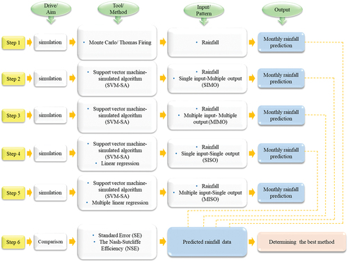
Figure 6 depicts the framework of this study in the form of a flowchart.

Figure 6. The framework of study identification and selection process.

Result

The time series of 34 rain gauge stations of the Karkheh basin was used to reconstruct and predict monthly rainfall. After the initial review of the monthly rainfall time series of the studied stations, 80% of the data of each time series was considered for calibration and 20% for validation. In the following, the performance of the models used in this study to reconstruct and predict monthly rainfall is considered.

Prediction by Monte Carlo and Thomas Fiering models

In this section, modeling and predicting were done in two stages. In the first step, using MINITAB (2014) software, the degree of autocorrelation between the statistics and information of the regional stations was investigated. In the next step, if the time series was independent, the Monte Carlo model was used, and otherwise, the Thomas Fiering model was used to predict the monthly rainfall statistics. Finally, monthly rainfall was predicted in the periods related to calibration and validation. For example, the results of calculating the statistical indicators of 10 rain gauge stations in the verification stage can be seen in Table 3, and the graph of observed values and values predicted by the model for one station can be seen in Figure 7. Upon examination of the figure, it is evident that the simulation results display deviations from the observed data at specific points, indicating discrepancies between the simulated and actual values. The validation results of this method show that the mean and standard deviation of the standard error of 34 rain gauge stations are 1.294 and 0.229, respectively. In this method, the results indicate that the Nash coefficient ranges from −0.672 to 0.391. Given that the Nash coefficient is less than 0.5, it suggests that the model has the low accuracyFiering in predicting monthly rainfall.

Figure 7. Comparison of observed and predicted rainfall in the validation stage by Monte Carlo and Thomas Fiering models at Sarabi rain gauge station.

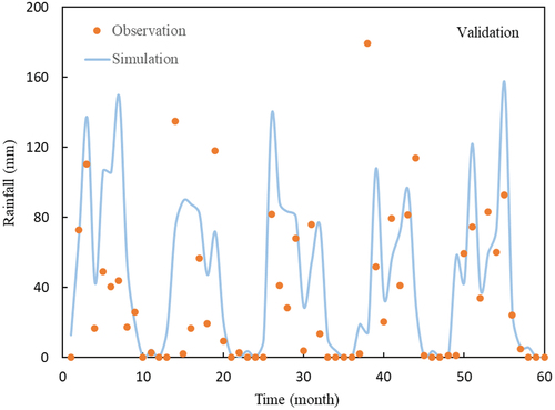
Table 3. The results related to the prediction of rainfall in the 10 studied rain gauge stations using the Monte Carlo and Thomas Fiering methods.

Station		Validation step
Row	Name	R^2	RMSE (mm)	SE	NSE
1	Afrine (Kashkan)	0.17	51.75	1.31	−0.03
2	Baba Pir Ali	0.23	38.34	1.19	0.11
3	Cham Anjir	0.23	48.75	1.31	−0.25
4	Cham Gaz	0.21	56.58	1.45	−0.27
5	Kaka Reza	0.16	66.35	1.47	−0.28
6	Kheir Abad	0.22	39.78	1.24	0.05
7	Pol Dokhtar	0.27	42.74	1.21	−0.01
8	Sarab Seyed Ali	0.22	50.66	1.24	−0.01
9	Sarabi	0.32	42.06	1.23	−0.03
10	Tang Siab	0.21	44.54	1.65	−0.58

Prediction by SVM-SA model based on SIMO method

Table 4 showcases the results of statistical indicator calculations during the calibration and validation stages for 10 rain gauge stations (for instance), while Figure 8 illustrates the graph comparing observed values and model-predicted values during the calibration and validation periods for one station. The results show varying levels of performance across different stations during both calibration and validation steps, suggesting differing predictive accuracy for rainfall at each location. The results indicate that the combined SVM-SA model based on the SIMO method achieved a mean standard error of 0.988 and a standard deviation of 0.246 for predicting monthly rainfall. However, the Nash coefficient in this model ranges from −1.13 to 0.60, suggesting poor performance.

Figure 8. Comparison of observed and predicted rainfall in the calibration and validation stage using SIMO method and with the help of SVM-SA model in Sarabi rain gauge station.

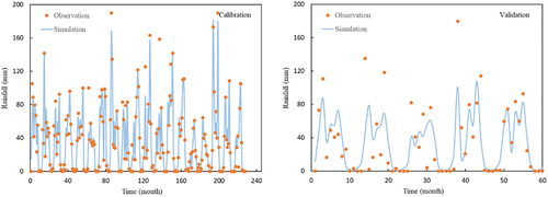
Table 4. Results related to rainfall predicting in 10 studied rain gauge stations by SIMO method and with the help of SVM-SA.

Station		Calibration step				Validation step
Row	Name	R^2	RMSE (mm)	SE	NSE	R^2	RMSE (mm)	SE	NSE
1	Afrine (Kashkan)	0.61	30.47	0.74	0.61	0.49	36.46	0.92	0.49
2	Baba Pir Ali	0.81	20.64	0.54	0.80	0.44	27.48	0.85	0.33
3	Cham Anjir	0.65	27.66	0.7	0.65	0.44	33.04	0.89	0.43
4	Cham Gaz	0.71	28.8	0.71	0.71	0.51	35.31	0.91	0.50
5	Kaka Reza	0.68	31.71	0.67	0.68	0.53	40.98	0.91	0.51
6	Kheir Abad	0.73	17.86	0.59	0.73	0.38	32.3	1.01	0.37
7	Pol Dokhtar	0.63	26.45	0.79	0.63	0.5	30.3	0.86	0.49
8	Sarab Seyed Ali	0.64	31.12	0.72	0.64	0.54	34.47	0.85	0.53
9	Sarabi	0.9	13.21	0.36	0.89	0.58	27.05	0.79	0.57
10	Tang Siab	0.64	26.44	0.75	0.63	0.45	26.44	0.98	0.44

Upon Figure 8, it is evident that the model demonstrates strong predictive capability and acceptable accuracy when applied to observational data during the calibration phase. However, during the validation phase, the model’s performance is notably poor, particularly in its inability to accurately estimate rainfall values exceeding 100 mm.

Comparing the results of Tables 3 and 4, it’s evident that the SIMO method with the SVM-SA model generally outperforms the Monte Carlo and Thomas Fiering methods in terms of R² and RMSE values for both the calibration and validation steps. The NSE values also show improvements in predictive accuracy for most of the stations when using the SIMO method with the SVM-SA model. This comparison highlights the potential effectiveness of the SIMO method with the SVM-SA model for rainfall prediction in the studied rain gauge stations.

Prediction by SVM-SA model based on the MIMO method

The statistical indicator calculations for the calibration and validation stages of 10 rain gauge stations (for example) are presented in Table 5 and the graph comparing observed values and model- predicted values for one station can be seen in Figure 9. It is evident that the calibration step generally demonstrates higher R² values and lower RMSE compared to the validation step. This indicates that the model performs better in predicting rainfall during the calibration phase than in the validation phase across the studied stations. Additionally, the NSE values provide insights into the model’s overall goodness-of-fit, with higher values indicating better model performance. The results show that the mean and standard deviation of the standard error of 34 rain gauge stations in the validation stage are 0.704 and 0.176, respectively. Also, the Nash coefficient in this model ranges from 0.018 to 0.835. When comparing the results from Table 4 (SIMO method) with Table 5 (MIMO method), it is evident that the MIMO method generally outperforms the SIMO method in both the calibration and validation steps. The MIMO method demonstrates higher R² values, lower RMSE in millimeters, and higher NSE values, indicating better predictive capability and accuracy compared to the SIMO method across the studied rain gauge stations.

Figure 9. Comparison of observed and predicted rainfall in the calibration and validation stage using MIMO method and with the help of SVM-SA model in Sarabi rain gauge station.

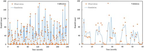
Table 5. Results related to rainfall predicting in 10 studied rain gauge stations by MIMO method and with the help of SVM-SA.

Station name			Calibration step				Validation step
Row	Dependent	Independent	R^2	RMSE (mm)	SE	NSE	R^2	RMSE (mm)	SE	NSE
1	Afrine (Kashkan)	Pol Dokhtar	0.95	11.06	0.27	0.95	0.80	23.8	0.61	0.79
2	Baba Pir Ali	Sarabi	0.92	12.05	0.34	0.92	0.77	20.32	0.55	0.77
3	Cham Anjir	Dehno	0.91	13.48	0.36	0.91	0.63	27.8	0.71	0.63
4	Cham Gaz	Jelogir	0.96	10.61	0.24	0.96	0.8	21.56	0.6	0.80
5	Kaka Reza	Sarab Seyed Ali	0.90	18.59	0.40	0.90	0.75	27.66	0.57	0.75
6	Kheir Abad	Sarabi	0.98	5.72	0.19	0.97	0.73	22	0.64	0.64
7	Pol Dokhtar	Afrine (Kashkan)	0.95	10.28	0.3	0.94	0.83	17.99	0.59	0.82
8	Sarab Seyed Ali	Kaka Reza	0.88	18.38	0.43	0.88	0.73	25.45	0.58	0.73
9	Sarabi	Kheir Abad	0.99	4.29	0.12	0.99	0.58	27.38	0.69	0.58
10	Tang Siab	Afrine (Kashkan)	0.90	13.86	0.42	0.89	0.84	16.56	0.49	0.84

Prediction by SVM-SA model based on the SISO method

For predicting monthly rainfall in this method, the SVM-SA model was also used. Prediction using the SVM-SA model, like MIMO and SIMO methods, was implemented in the MATLAB (2017) environment. As an example, the results of calculating the statistical indicators in the two stages of calibration and validation of 10 rain gauge stations can be seen in Table 6, respectively, and the graphs of observed values and predicted values for one station can be seen in Figure 10. The results show that the mean and standard deviation of the standard error of the SVM-SA model for 34 stations are 0.537 and 0.167, respectively. Figure 10 illustrates the model’s strong predictive capability and acceptable accuracy when applied to observed data in both the calibration and validation phases. The model effectively predicts precipitation amounts at the time of occurrence in both phases. As indicated in Table 6, the minimum Nash coefficient values of 0.77 for the calibration phase and 0.74 for the validation period confirm the model’s high accuracy in predicting rainfall at different stations.

Figure 10. Comparison of observed and predicted rainfall in the calibration and validation stage using SISO method and with the help of SVM-SA model in Sarabi rain gauge station.

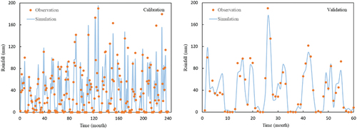
Table 6. Results related to rainfall prediction in 10 studied rain gauge stations by the SISO method and with the help of SVM-SA.

Station name			Calibration step				Validation step
Row	Dependent	Independent	R^2	RMSE (mm)	SE	NSE	R^2	RMSE (mm)	SE	NSE
1	Afrine (Kashkan)	Pol Dokhtar	0.91	14.94	0.36	0.91	0.91	16.5	0.42	0.90
2	Baba Pir Ali	Sarabi	0.83	17.65	0.5	0.83	0.89	14.34	0.39	0.89
3	Cham Anjir	Dehno	0.77	21.32	0.57	0.77	0.74	23.42	0.6	0.74
4	Cham Gaz	Jelogir	0.88	19.23	0.44	0.88	0.8	21.85	0.6	0.79
5	Kaka Reza	Sarab Seyed Ali	0.78	27.05	0.58	0.78	0.84	22.67	0.46	0.83
6	Kheir Abad	Sarabi	0.93	9.58	0.31	0.93	0.89	12.5	0.36	0.88
7	Pol Dokhtar	Afrine (Kashkan)	0.9	13.96	0.4	0.90	0.87	16.88	0.55	0.84
8	Sarab Seyed Ali	Kaka Reza	0.78	24.54	0.57	0.78	0.85	18.88	0.43	0.85
9	Sarabi	Kheir Abad	0.93	10.61	0.3	0.93	0.92	12.04	0.3	0.92
10	Tang Siab	Afrine (Kashkan)	0.83	17.5	0.52	0.83	0.82	17.35	0.51	0.82

According to the results and its comparison with the SIMO and MIMO methods, it can be stated that the use of the rainfall statistics of an independent station in this method, like the MIMO method, has led to an increase in the model’s accuracy. We should note that the use of rainfall statistics based on the order of occurrence time in the SISO method has improved the performance of the model.

Prediction by LR model based on the SISO method

In this method, the LR model was used to predict monthly rainfall. As an example, the results of calculating the statistical indicators of the model in the calibration and validation stage of 10 rain gauge stations can be seen in Table 7, respectively, and the graphs of observed values and values predicted by the model for one station can be seen in Figure 11. The results show that the mean and standard deviation of the standard error of the LR model are 0.517 and 0.160, respectively. Also, the Nash coefficient in this model ranges from 0.601 to 0.919. The results indicate that the simulation model generally performs well, with most stations achieving relatively high R² and NSE values and low RMSE and SE values. Upon comparing the results in Table 6 with those in Table 7, along with Figures 10 and 11, it becomes apparent that the LR model generally outperforms the SVM-SA model in the SISO method. The LR model demonstrates effective prediction of high rainfall amounts, indicating superior predictability and accuracy compared to the SVM-SA model across the studied rain gauge stations.

Figure 11. Comparison of observed and predicted rainfall in the calibration and validation stage using SISO method and with the help of LR model in Sarabi rain gauge station.

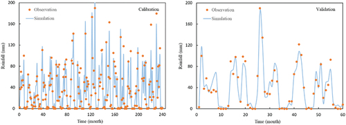
Table 7. Results related to rainfall predicting in 10 studied rain gauge stations by SISO method and with the help of LR.

	Station name		Calibration step				Validation step
Row	Dependent	Independent	R^2	RMSE (mm)	SE	NSE	R^2	RMSE (mm)	SE	NSE
1	Afrine (Kashkan)	Pol Dokhtar	0.9	15.65	0.38	0.90	0.91	16.42	0.42	0.90
2	Baba Pir Ali	Sarabi	0.83	17.65	0.5	0.83	0.89	14.33	0.39	0.89
3	Cham Anjir	Dehno	0.74	22.68	0.6	0.74	0.75	22.91	0.59	0.75
4	Cham Gaz	Jelogir	0.86	20.85	0.48	0.86	0.79	22.02	0.61	0.79
5	Kaka Reza	Sarab Seyed Ali	0.77	27.47	0.59	0.77	0.84	22.72	0.46	0.83
6	Kheir Abad	Sarabi	0.93	9.57	0.31	0.93	0.92	10.39	0.3	0.92
7	Pol Dokhtar	Afrine (Kashkan)	0.9	13.96	0.4	0.90	0.91	13.41	0.44	0.90
8	Sarab Seyed Ali	Kaka Reza	0.77	25.15	0.58	0.77	0.84	19.5	0.45	0.84
9	Sarabi	Kheir Abad	0.93	10.78	0.31	0.93	0.92	11.81	0.3	0.92
10	Tang Siab	Afrine (Kashkan)	0.83	17.56	0.53	0.83	0.82	17.45	0.51	0.82

Prediction by SVM-SA model based on the MISO method

In this model, the time series statistics of three stations were used to predict and reconstruct the monthly rainfall, so the time series statistics of two stations were used as independent stations and the time series statistics of one station were used as dependent stations. As an example, the results of the calculation of statistical indicators in the validation stage of 10 rain gauge stations can be seen in Table 8 and the graph of observed values and values predicted by the model for one station can be seen in Figure 12. The results show that the mean and standard deviation of the standard error of the SVM-SA model are 0.544 and 0.179, respectively. Figure 12 clearly demonstrates the model’s robust predictive ability and satisfactory accuracy when applied to observational data during both the calibration and validation phases, even for high rainfall levels. Table 8 further emphasizes the model’s high accuracy, with Nash coefficients ranging from 0.78 to 0.94 in the calibration phase and from 0.74 to 0.93 in the validation phase, confirming its effectiveness in rainfall prediction.

Figure 12. Comparison of observed and predicted rainfall in the calibration and validation stage using the MISO method and with the help of the SVM-SA model at the Sarabi rain gauge station.

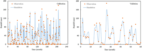
Table 8. The results related to rainfall predicting in 10 studied rain gauge stations using the MISO method and with the help of SVM-SA.

	Station name			Calibration step				Validation step
Row	Dependent	Independent	Independent	R^2	RMSE (mm)	SE	NSE	R^2	RMSE (mm)	SE	NSE
1	Afrine (Kashkan)	Pol Dokhtar	Tang Siab	0.92	14.2	0.34	0.92	0.90	14.5	0.39	0.90
2	Baba Pir Ali	Sarabi	Kheir Abad	0.83	17.68	0.50	0.83	0.86	15.85	0.41	0.92
3	Cham Anjir	Kaka Reza	Sarab Seyed Ali	0.86	18.04	0.45	0.86	0.81	17.94	0.54	0.79
4	Cham Gaz	Jelogir	Pol Zal	0.94	13.74	0.31	0.94	0.92	17.33	0.39	0.91
5	Kaka Reza	Cham Anjir	Dehno	0.82	23.83	0.51	0.78	0.67	28.22	0.7	0.74
6	Kheir Abad	Baba Pir Ali	Sarabi	0.93	8.93	0.31	0.93	0.92	10.12	0.29	0.92
7	Pol dokhtar	Afrine (Kashkan)	Tang Siab	0.92	12.34	0.36	0.92	0.88	14.06	0.45	0.88
8	Sarab Seyed Ali	Cham Anjir	Kaka Reza	0.87	18.5	0.43	0.87	0.87	16.48	0.41	0.86
9	Sarabi	Baba Pir Ali	Kheir Abad	0.94	9.63	0.28	0.94	0.93	11.05	0.28	0.93
10	Tang Siab	Pol Dokhtar	Afrine (Kashkan)	0.84	16.81	0.50	0.86	0.82	17.27	0.54	0.82

By examining the results of Monte Carlo and Thomas Fiering, SIMO, MIMO, SISO, and MISO methods, it can be seen that the use of rainfall statistics of independent stations in the reconstruction and predicting of rainfall in MIMO, SISO, and MISO methods increase the accuracy of the model compared to Monte Carlo and Thomas Fiering methods. Also, the results of MIMO, SISO, and MISO show that the use of time series statistics in the order of occurrence leads to an increase in accuracy. Finally, the comparison of the results of the MISO and SISO methods shows that the use of an independent station in predicting monthly rainfall with the SISO method has performed better in predicting monthly rainfall.

Prediction by MLR model based on the MISO method

This model was implemented in SPSS software. The statistical indicators calculated during the verification stage for 10 rain gauge stations are detailed in Table 9, and a graph depicting observed values versus model-predicted values for a specific station is provided in Figure 13. The mentioned figure demonstrates the method’s capability to accurately simulate observed peak and trough events. The results show that the mean and standard deviation of the standard error of the linear regression model are 0.531 and 0.173, respectively. The Nash coefficient in this model ranges from 0.533 to 0.959. By comparing the results of the multiple linear regression model with the SVM-SA model based on the MISO method, it can be seen that the multiple linear regression model performed better than the SVM-SA model in predicting monthly rainfall.

Figure 13. Comparison of observed and predicted rainfall in the calibration and validation stage using the MISO method and with the help of the MLR model at the Sarabi rain gauge station.

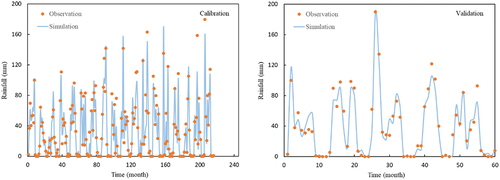
Table 9. The results related to rainfall predicting in the 10 studied rain gauge stations using the MISO method and with the help of MLR.

	Station name			Calibration step				Validation step
Row	Dependent	Independent	Independent	R^2	RMSE (mm)	SE	NSE	R^2	RMSE (mm)	SE	NSE
1	Afrine (Kashkan)	Pol Dokhtar	Tang Siab	0.92	14.2	0.34	0.92	0.90	14.5	0.39	0.90
2	Baba Pir Ali	Sarabi	Kheir Abad	0.83	17.68	0.50	0.83	0.86	15.85	0.41	0.92
3	Cham Anjir	Kaka Reza	Sarab Seyed Ali	0.86	18.04	0.45	0.85	0.81	17.94	0.54	0.80
4	Cham Gaz	Jelogir	Pol Zal	0.94	13.74	0.31	0.90	0.92	17.33	0.39	0.88
5	Kaka Reza	Cham Anjir	Dehno	0.82	23.83	0.51	0.73	0.67	28.22	0.7	0.72
6	Kheir Abad	Baba Pir Ali	Sarabi	0.93	8.93	0.31	0.93	0.92	10.12	0.29	0.96
7	Pol dokhtar	Afrine (Kashkan)	Tang Siab	0.92	12.34	0.36	0.92	0.88	14.06	0.45	0.88
8	Sarab Seyed Ali	Cham Anjir	Kaka Reza	0.87	18.5	0.43	0.87	0.87	16.48	0.41	0.92
9	Sarabi	Baba Pir Ali	Kheir Abad	0.94	9.63	0.28	0.93	0.93	11.05	0.28	0.94
10	Tang Siab	Pol Dokhtar	Afrine (Kashkan)	0.84	16.81	0.50	0.84	0.82	17.27	0.54	0.83

To choose the best method and model, we present the summary of monthly rainfall prediction results in Table 10. According to the results, it can be seen that classical, SIMO, and MIMO methods have an average error of over 0.5 and perform poorly in monthly rainfall predicting compared with SISO and MISO methods. Also, the results show that there is no significant difference between the SISO and MISO methods, but the SISO method and the LR model have the best performance among other methods with an average and standard deviation of 0.517 and 0.160 and are more accurate in predicting monthly rainfall.

Table 10. Average indicators related to monthly rainfall prediction in the studied rain gauge stations.

Method	Model	Ave SE	Std SE
Classic	Monte Carlo/Thomas Firing	1.29	0.23
SIMO	SVM-SA	0.99	0.25
MIMO	SVM-SA	0.70	0.18
SISO	SVM-SA	0.54	0.17
	LR	0.52	0.16
MISO	SVM-SA	0.54	0.18
	MLR	0.53	0.17

Conclusion

In this study, the accuracy and efficiency of the SVM-SA model based on the SIMO, MIMO, SISO, and MISO methods and the classic Thomas Fiering and Monte Carlo models were investigated. We got the following results:

By examining the performance of the Monte Carlo and Thomas Fiering and model, it can be stated that this model had a poor performance and is not recommended for predicting monthly rainfall.

The SIMO method is relatively more accurate compared to the classical model. By comparing the results of the MIMO and SIMO methods, it can be seen that the MIMO method has a higher accuracy in predicting monthly rainfall with a lower average and standard deviation of the standard error.

In the SISO method, although, to compare the results, it can be stated that there is no significant difference between the SVM-SA and LR models, but the LR model has a lower average standard error and is easier than the SVM-SA model to predict rainfall.

In the MISO method, to compare the results, we can see that there is no significant difference between the SVM-SA and MLR models. But it can be said that the MLR model can predict more easily and in less time because of having a lower average error and also having less adjustable parameters than the SVM-SA model, and in this sense, it is preferable to other models.

MIMO, SISO, and MISO methods have higher accuracy in reconstructing and predicting monthly rainfall than SIMO and Monte Carlo and Thomas Fiering methods due to the use of statistics from other stations as independent stations.

Among the predicting methods studied, SISO, MISO, MIMO, SIMO, and Monte Carlo and Thomas Fiering methods are ranked first to fifth, respectively.

By examining the acceptable results of this research, we can see that there is no significant difference between the mentioned methods and models, and they can be used in research according to the data. But the general results indicate that the SISO method can predict more easily and in less time because of the use of statistics from other stations as an independent station and the LR model, because of having an average standard error and less adjustable parameters, and in this respect compared to other models are preferred and recommended.

The extensive use of 34 meteorological stations in this research indicates the potential strength of these methods for application in other stations and their generalization to stations in different basins. However, conducting validation experiments in multiple watersheds with diverse characteristics would further support the broader applicability of the research.

Disclosure statement

No potential conflict of interest was reported by the author(s).

References

- Abdullah, A. S., Ruchjana, B. N., Jaya, I. G. N. M., (2021). Comparison of SARIMA and SVM model for rainfall forecasting in Bogor city, Indonesia. Journal of Physics: Conference Series, 1722(1), 012061. doi:10.1088/1742-6596/1722/1/012061
- Abebe, W. T., & Endalie, D. (2023). Artificial intelligence models for prediction of monthly rainfall without climatic data for meteorological stations in Ethiopia. Journal of Big Data, 10(1), 2. doi:10.1186/s40537-022-00683-3
- Ahmadi, F., Radmanesh, F., & Mir Abbasi Najafabadi, R. (2013). Comparison of genetic programming methods and support vector machine in predicting daily river flow in barandozchai river. Soil and Water Research, 28, 1171–1162.
- Amisigo, B. A., Van de Giesen, N., Rogers, C., Andah, W. E. I., & Friesen, J. (2008). Monthly streamflow prediction in the volta basin of West Africa: A SISO NARMAX polynomial modelling. Physics and Chemistry of the Earth, 33(1–2), 141–15. doi:10.1016/j.pce.2007.04.019
- Arriagada, P., Dieppois, B., Sidibe, M., & Link, O. (2019). Impacts of climate change and climate variability on hydropower potential in data-scarce regions subjected to multi-decadal variability. Energies, 12(14), 2747. doi:10.3390/en12142747
- Arselan, C. A. (2012). Stream flow simulation and synthetic flow calculation by modified Thomas Fiering model. Al-Rafidain Engineering Journal, 20(4), 118–127. doi:10.33899/rengj.2012.54160
- Azadi, S., Nozari, H., & Godarzi, E. (2020). Predicting sediment load using stochastic model and rating curves in a hydrological station. Journal of Hydrologic Engineering, 25(8), 05020017. doi:10.1061/(ASCE)HE.1943-5584.0001967
- Azadi, M., Taghizadeh, E., Memarian, M. H., & Dmitrieva-Arrago, L. R. (2013). Comparing the results of precipitation forecast based on mesoscale models on the territory of Iran during the cold season. Russian Meteorology and Hydrology, 38(9), 605–613. doi:10.3103/S1068373913090033
- Bashar, A. M., Nozari, H., Marofi, S., Mohamadi, M., & Ahadiiman, A. (2023). Investigation of factors affecting rural drinking water consumption using intelligent hybrid models. Water Science and Engineering, 16(2), 175–183. doi:10.1016/j.wse.2022.12.002
- Behzad, M., Asghari, K., & Coppola, E. A., Jr. (2010). Comparative study of SVMs and ANNs in aquifer water level prediction. Journal of Computing in Civil Engineering, 24(5), 408–413. doi:10.1061/(ASCE)CP.1943-5487.0000043
- Benimam, H., Si-Moussa, C., Laidi, M., & Hanini, S. (2020). Modeling the activity coefficient at infinite dilution of water in ionic liquids using artificial neural networks and support vector machines. Neural Computing & Applications, 32(12), 8635–8653. doi:10.1007/s00521-019-04356-w
- Cercignani, C. (1988). The Boltzmann equation. In the Boltzmann equation and its applications (pp. 40–103). New York: Springer.
- Choubin, B., Khalighi-Sigaroodi, S., Malekian, A., & Kis¸i, Ö. (2016). Multiple linear regression, multi-layer perceptron network and adaptive neuro-fuzzy inference system for forecasting precipitation based on large-scale climate signals. Hydrological Sciences Journal, 61(6), 1001–1009. doi:10.1080/02626667.2014.966721
- Danandeh Mehr, A., Nourani, V., Karimi Khosrowshahi, V., & Ghorbani, M. A. (2019). A hybrid support vector regression–firefly model for monthly rainfall forecasting. International Journal of Environmental Science and Technology, 16(1), 335–346. doi:10.1007/s13762-018-1674-2
- Dawoodi, H. H. (2021). Rainfall prediction in north Maharashtra region using support vector machine. TURCOMAT, 12(7), 1501–1505.
- Du, J., Liu, Y., Yu, Y., & Yan, W. (2017). A prediction of precipitation data based on support vector machine and particle swarm optimization (PSO-SVM) algorithms. Algorithms, 10(2), 57. doi:10.3390/a10020057
- Galelli, S., & Castelletti, A. (2013). Tree‐based iterative input variable selection for hydrological modeling. Water Resources Research, 49(7), 4295–4310. doi:10.1002/wrcr.20339
- Giang, N. H., Wang, Y., Hieu, T. D., Phuong, L. A., & Thinh, N. T. (2022). Monthly precipitation prediction using neural network algorithms in the thua Thien hue province. Journal of Water and Climate Change, 13(5), 2011–2033. doi:10.2166/wcc.2022.271
- Hamidi, O., Poorolajal, J., Sadeghifar, M., Abbasi, H., Maryanaji, Z., Faridi, H. R., & Tapak, L. (2015). A comparative study of support vector machines and artificial neural networks for predicting precipitation in Iran. Theoretical and Applied Climatology, 119(3–4), 723–731. doi:10.1007/s00704-014-1141-z
- Iranian Water Resources Management Company. 2022. Data center. Available from: http://wrbs.wrm.ir.
- Kisi, O., & Cimen, M. (2012). Precipitation forecasting by using wavelet-support vector machine conjunction model. Engineering Applications of Artificial Intelligence, 25(4), 783–792. doi:10.1016/j.engappai.2011.11.003
- Kisi, O., & Ozkan, C. (2017). A new approach for modeling sediment-discharge relationship: Local weighted linear regression. Water Resources Management, 31(1), 1–23. doi:10.1007/s11269-016-1481-9
- Lin, S. S., Zhang, N., Zhou, A., & Shen, S. L. (2022). Time-series prediction of shield movement performance during tunneling based on hybrid model. Tunn Undergr Space Technol, 119, 104245. doi:10.1016/j.tust.2021.104245
- Markuna, S., Kumar, P., Ali, R., Vishwkarma, D. K., Kushwaha, K. S. … Kuriqi, A. (2023). Application of innovative machine learning techniques for long-term rainfall prediction. Geofisica Pura E Applicata, 180(1), 335–363. doi:10.1007/s00024-022-03189-4
- Moharana, L., Sahoo, A., & Ghose, D. K. (2022). Prediction of rainfall using hybrid SVM-HHO model. IOP conf. Ser Earth Environmental Sciences, 1084(1), 012054. doi:10.1088/1755-1315/1084/1/012054
- Nasir, H. A., & Weyer, E. (2016). System identification of the upper part of Murray River. Control Engineering Practice, 52, 70–92. doi:10.1016/j.conengprac.2016.04.006
- Novak, D. R., Bailey, C., Brill, K. F., Burke, P., Hogsett, W. A., Rausch, R., & Schichtel, M. (2014). Precipitation and temperature forecast performance at the weather prediction center. Weather Forecast, 29(3), 489–504. doi:10.1175/WAF-D-13-00066.1
- Nozari, H., & Tavakoli, F. (2020). Forecasting hydrologic parameters using linear and nonlinear stochastic models. Journal of Water and Climate Change, 11(4), 1284–1301. doi:10.2166/wcc.2019.249
- Ortiz-García, E. G., Salcedo-Sanz, S., & Casanova-Mateo, C. (2014). Accurate precipitation prediction with support vector classifiers: A study including novel predictive variables and observational data. Atmospheric Research, 139, 128–136. doi:10.1016/j.atmosres.2014.01.012
- Pai, P. F., & Hong, W. C. (2007). A recurrent support vector regression model in rainfall forecasting. Hydrological Processes: International Journal, 21(6), 819–827. doi:10.1002/hyp.6323
- Park, K., Rothfeder, R., Petheram, S., Buaku, F., Ewing, R., & Greene, W. H. (2020). Linear regression. In R. Ewing & K. Park (Eds.), Basic Quantitative Research Methods for Urban Planners (pp. 220–269). New York: Routledge.
- Parmar, A., Mistree, K., & Sompura, M., 2017. Machine learning techniques for rainfall prediction: A review. In International conference on innovations in information embedded and communication systems, Coimbatore, India, 17–18 March 2017.
- Patra, T., Mitra, S. K., & Pinchera, D. (2020). Link Budget Analysis for 5G communication in the Tropical Regions. Wireless Communications and Mobile Computing, 2020, 1–9. doi:10.1155/2020/6669965
- Pham, B. T., Le, L. M., Le, T. T., Bui, K. T. T., Le, V. M., Ly, H. B., & Prakash, I. (2020). Development of advanced artificial intelligence models for daily rainfall prediction. Atmospheric Research, 237, 104845. doi:10.1016/j.atmosres.2020.104845
- Pouyanfar, S., Nozari, H., & Khodamorad Pour, M. (2023). Comparison of the performances of the gene expression programming model and the RegCM model in predicting monthly runoff. Journal of Water and Climate Change, 14(10), 3810–3829. doi:10.2166/wcc.2023.439
- Rahimi, N., Arian, M., & Ghorashi, M. (2017). Active tectonics of the saymareh-karkheh river basin (Northwest of Persian Gulf, Iran). Open Journal of Marine Science, 7(2), 238–257. doi:10.4236/ojms.2017.72017
- Reddy, P. C. S., Yadala, S., & Goddumarri, S. N. (2022). Development of rainfall forecasting model using machine learning with singular spectrum analysis. IIUM Engineering Journal, 23(1), 172–186. doi:10.31436/iiumej.v23i1.1822
- Ren, Y., Hu, F., & Miao, H. (2016). The optimization of kernel function and its parameters for SVM in well-logging, 13th International Conference on Service Systems and Service Management (ICSSSM), Kunming, China, (pp. 1–5). ICSSSM., IEEE. doi: 10.1109/ICSSSM.2016.7538563
- Rosen, S. L., & Harmonosky, C. M. (2005). An improved simulated annealing simulation optimization method for discrete parameter stochastic systems. Computers & Operations Research, 32(2), 343–358. doi:10.1016/S0305-0548(03)00240-5
- Safari, M. J. S., Rahimzadeh Arashloo, S., & Danandeh Mehr, A. (2020). Rainfall-runoff modeling through regression in the reproducing kernel Hilbert space algorithm. Journal of Hydrology, 587, 125014. doi:10.1016/j.jhydrol.2020.125014
- Sehad, M., Lazri, M., & Ameur, S. (2017). Novel SVM-based technique to improve rainfall estimation over the Mediterranean region (north of Algeria) using the multispectral MSG SEVIRI imagery. Advances in Space Research, 59(5), 1381–1394. doi:10.1016/j.asr.2016.11.042
- Shao, Q., & Li, M. (2013). An improved statistical analogue downscaling procedure for seasonal precipitation forecast. Stochastic Environmental Research and Risk Assessment, 27(4), 819–830. doi:10.1007/s00477-012-0610-0
- Shenify, M., Danesh, A. S., Gocić, M., Taher, R. S., Abdul Wahab, A. W., Gani, A., & Petković, D. (2016). Precipitation estimation using support vector machine with discrete wavelet transform. Water Resource Management, 30(2), 641–652. doi:10.1007/s11269-015-1182-9
- Sh, A., Khan, I. H., & Parida, B. P. (2001). Performance of stochastic approaches for forecasting river water quality. Water Research, 35(18), 4261–4266. doi:10.1016/S0043-1354(01)00167-1
- Silvestro, F., & Rebora, N. (2014). Impact of precipitation forecast uncertainties and initial soil moisture conditions on a probabilistic flood forecasting chain. Journal of Hydrology, 519, 1052–1067. doi:10.1016/j.jhydrol.2014.07.042
- Stanton, J. M., & Galton, P. (2001). The peas: A brief history of linear regression for statistics instructors. Journal of Statistics Education: An International Journal on the Teaching and Learning of Statistics, 9(3), 1–13. doi:10.1080/10691898.2001.11910537
- Subasi, A. (2013). Classification of EMG signals using PSO optimized SVM for diagnosis of neuromuscular disorders. Computers in Biology and Medicine, 43(5), 576–586. doi:10.1016/j.compbiomed.2013.01.020
- Tanessong, R. S., Igri, P. M., Vondou, D. A., Tamo, P. H. K., & Kamga, F. M. (2014). Evaluation of probabilistic precipitation forecast determined from WRF forecasted amounts. Theoretical and Applied Climatology, 116(3–4), 649–659. doi:10.1007/s00704-013-0965-2
- Tao, H., Sulaiman, S. O., Yaseen, Z. M., Asadi, H., Meshram, S. G., & Ghorbani, M. A. (2018). What is the potential of integrating phase space reconstruction with SVM-FFA data-intelligence model? Application of rainfall forecasting over regional scale. Water Resources Management, 32(12), 3935–3959. doi:10.1007/s11269-018-2028-z
- Tran, N. H., & Tran, K. (2007). Combination of fuzzy ranking and simulated annealing to improve discrete fracture inversion. Mathematical and Computer Modelling of Dynamical Systems, 45(7–8), 1010–1020. doi:10.1016/j.mcm.2006.08.013
- Wang, H., Shangguan, L., Wu, J., & Guan, R. (2013). Multiple linear regression modeling for compositional data. Neurocomputing, 122, 490–500. doi:10.1016/j.neucom.2013.05.025
- Yan, X., & Su, X. (2009). Linear regression analysis: Theory and computing. World Scientific, Singapore: World Scientific Research.
- Yu, P. S., Chen, S. T., & Chang, I. F. (2006). Support vector regression for real-time flood stage forecasting. Journal of Hydrology, 328(3–4), 704–716. doi:10.1016/j.jhydrol.2006.01.021
- Zaini, N., Malek, M. A., Yusoff, M., Mardi, N. H., & Norhisham, S. (2018). Daily river flow forecasting with hybrid support vector machine–particle swarm optimization. IOP Conference Series: Earth and Environmental Science, 140, 012035. doi:10.1088/1755-1315/140/1/012035
- Zhang, X., Chen, X., & He, Z. (2010). An ACO-based algorithm for parameter optimization of support vector machines. Expert Systems with Applications, 37(9), 6618–6628. doi:10.1016/j.eswa.2010.03.067